Machine Learning for Program Repair
When writing programs, a lot of time is spent debugging or fixing source code errors, both for beginners (imagine the intro programming classes you took) as well as for professional developers (for example, this case study from Google 1). Automating program repair could dramatically enhance the productivity of both programming and learning programming. In our recent work published at ICML 2020, we study how to use machine learning to repair programs automatically.
Problem Setting
Programmers write programs incrementally: write code, compile or execute it, and if there are any errors, repair the program based on the received feedback. Can we model and solve this problem with machine learning?
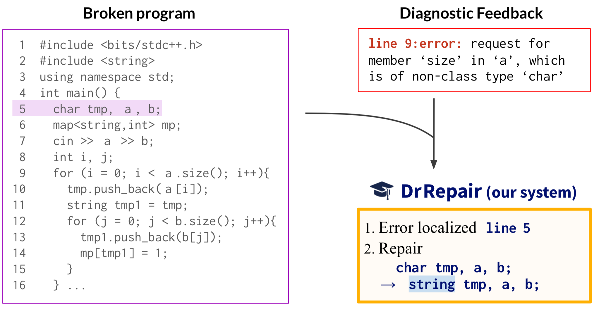
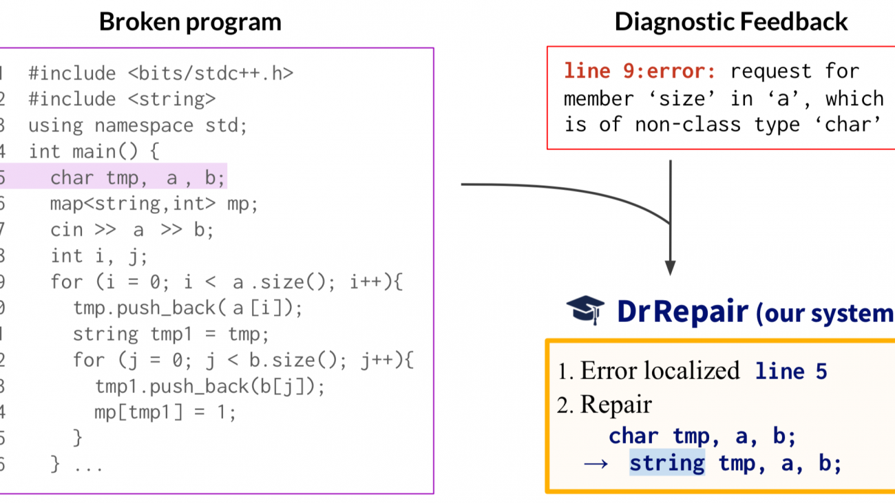
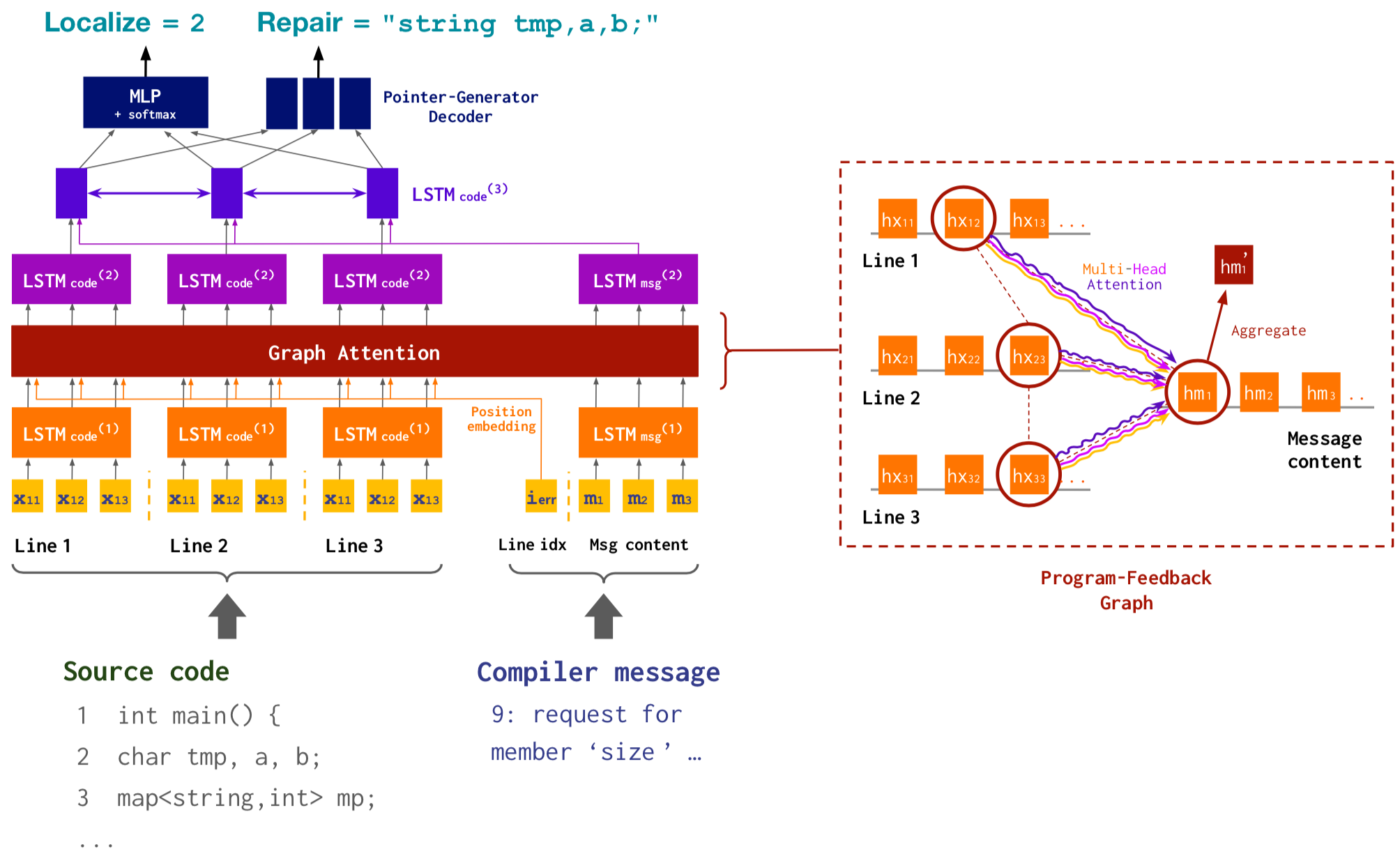
Let’s say we have a broken C++ program (figure left), where the char in line 5 should actually be string. When we compile it, we get an error (figure top right), which says “line 9 is requesting for size in a which is of type char”. From this message, a programmer can notice that the error is related to the type of the variable a, track how a has been used or declared in the source code, reaching line 5, and then edit the line to fix the error. Thus, the concrete task we want our machine learning model to solve is, given broken code (figure left) and an error message (figure top right), localize the error line (line 5) and generate a repaired version of it (“string tmp, a, b;”) (figure bottom right).
Challenges:
This task poses two main challenges. First, on the modeling side, we need to connect and jointly reason over two modalities, the program and the error message: for instance, tracking variables that caused the error as we saw in the example above. Second, on the training data side, we need an efficient source of data that provides supervision for correcting broken programs; unfortunately, existing labeled datasets with <broken code, fixed code> pairs are small and hard to come by, and don’t scale up. In this work, we introduce promising solutions to those two challenges by: 1) modeling program repair with program-feedback graph, and 2) introducing a self-supervised training scheme that uses unlabeled programs.
Modeling Approach: Program-Feedback Graph
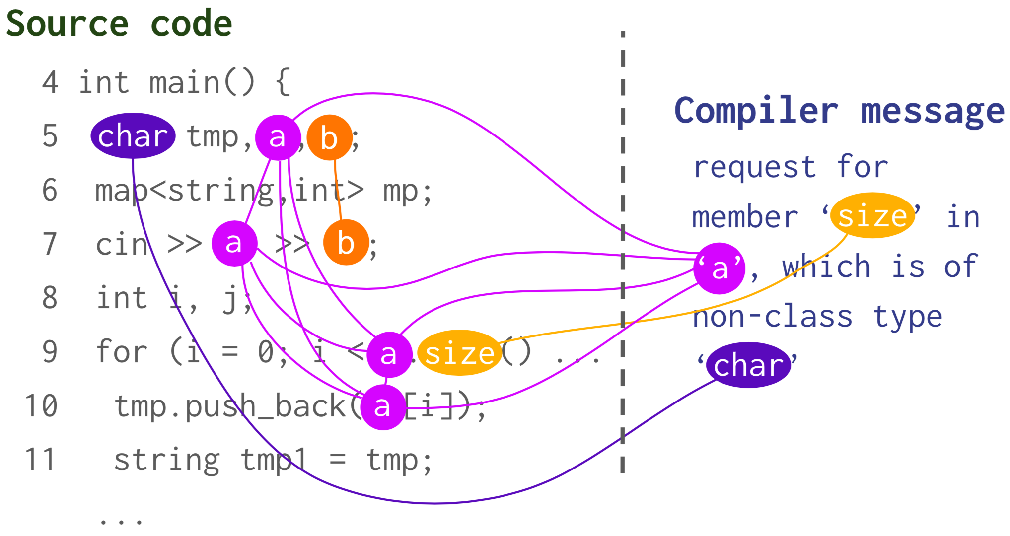
How can we effectively connect the two modalities (programs and error messages) and perform the reasoning needed for repair? To achieve this, we introduce a program-feedback graph, a joint graph representation that connects symbols across the program and error message. For instance, the compiler message in the example mentions a, size, and char, so we connect these symbols to their occurrences in the source code, to capture semantic correspondence. This way, we treat the two modalities in a shared semantic space rather than separately. We then perform reasoning over the symbols in this space using graph attention 2.
Specifically, for the model architecture, we build on the encoder-decoder framework commonly used in NLP, which encodes input sequences (in our case, the program and error message; next figure bottom) and then decodes outputs (in our case, the localized line index, and the repaired version of the line; figure top), and we incorporate a graph attention module applied to the program-feedback graph in the intermediate layer of the architecture (figure middle).
Training Approach: Self-Supervised Learning
Our second technique is self-supervised learning. Labeled datasets of program repair are small, but there are vast amounts of unlabeled programs available online. For example, GitHub has more than 30M public repositories. Using this large amount of freely available code to improve learning program repair would significantly enhance the scalability and reliability of our system.
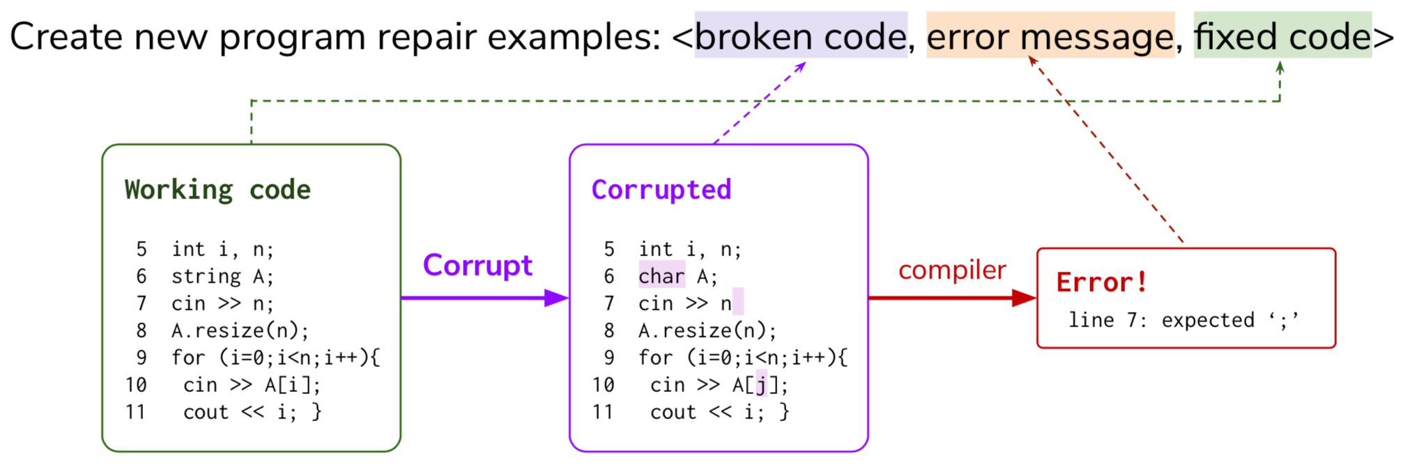
Our idea is as follows: we first collect unlabeled, working programs from online resources such as GitHub and codeforce.com (figure left). We then design randomized program corruption procedures (e.g. delete/insert/replace tokens) and corrupt the unlabeled programs (figure middle). As a result, the corrupted programs give us errors (figure right). This way, we can create a lot of new examples of program repair, <broken code, error message, fixed code>. We can use this extra data to pre-train the program repair model, and then fine-tune on the labeled target dataset.
Let’s use our program repair model!
We apply and evaluate our repair model (we call DrRepair) on two benchmark tasks:
- Correcting C programs written by students (DeepFix dataset3)
- Correcting the output of C++ program synthesis (SPoC dataset4)
Application to DeepFix (Correcting Student Programs)
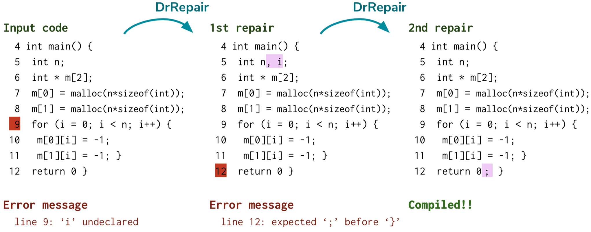
In DeepFix, the task is to correct C programs written by students in an intro programming class so that they will compile. The input programs may have multiple lines with errors, so we apply the repair model iteratively, addressing one error at a time. For instance, the following figure shows an example program in DeepFix, which has a compiler error saying that “i is undeclared”. By applying the repair model, DrRepair, it repairs this error by inserting a declaration of i in line 5. After this fix, we notice that there is another error, which says “expected semicolon before brace”. We can apply the repair model again – this time, the model inserts a semicolon in line 12, and now the repaired program compiles successfully! This approach is conducive to the idea of iterative refinement: we can keep running the repair model and progressively fixing errors.
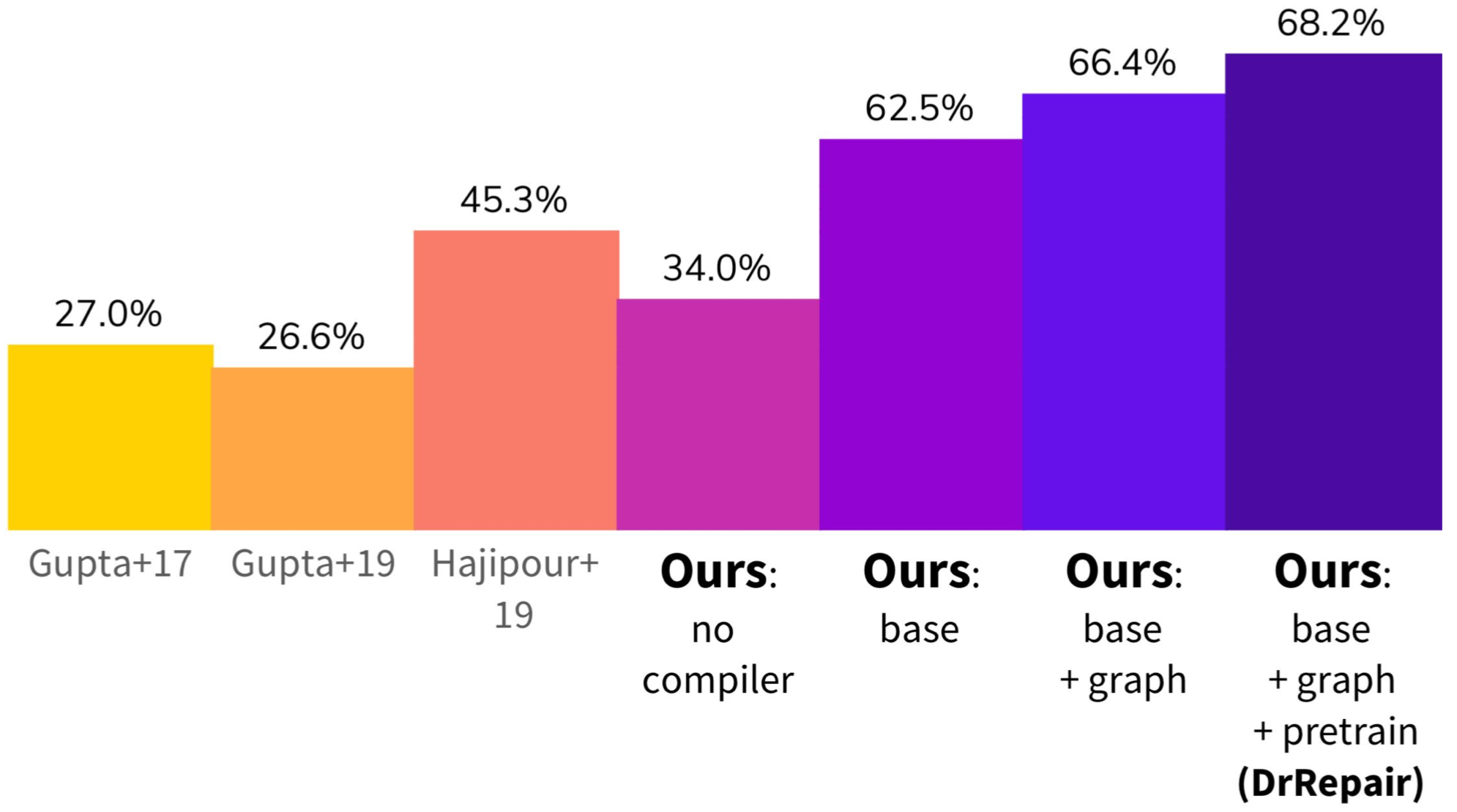
What is the effect of using error messages, program-feedback graphs, and self-supervised pre-training? Existing repair systems studied on DeepFix did not use compiler error messages – they aimed to directly translate from broken code to fixed code. To see the effect of using error messages in the first place, we tried removing all our techniques from the system: the use of compiler messages, program-feedback graphs, and pre-training. This version of our model (“ours: no compiler” in the figure below) achieves 34% repair accuracy on DeepFix, which is comparable to the existing systems. Now we add compiler messages to our input. We find that this model achieves much better performance and generalization (62.5% accuracy; “ours: base” in the figure). This suggests that with an access to error messages, the model learns the right inductive bias to repair the code based on the feedback. Next, we add program-feedback graphs and self-supervised pre-training. We find that both provide further improvements (“ours: base+graph” and “ours: base+graph+pretrain”), and our final system can fix 68.2% of the broken programs in DeepFix!
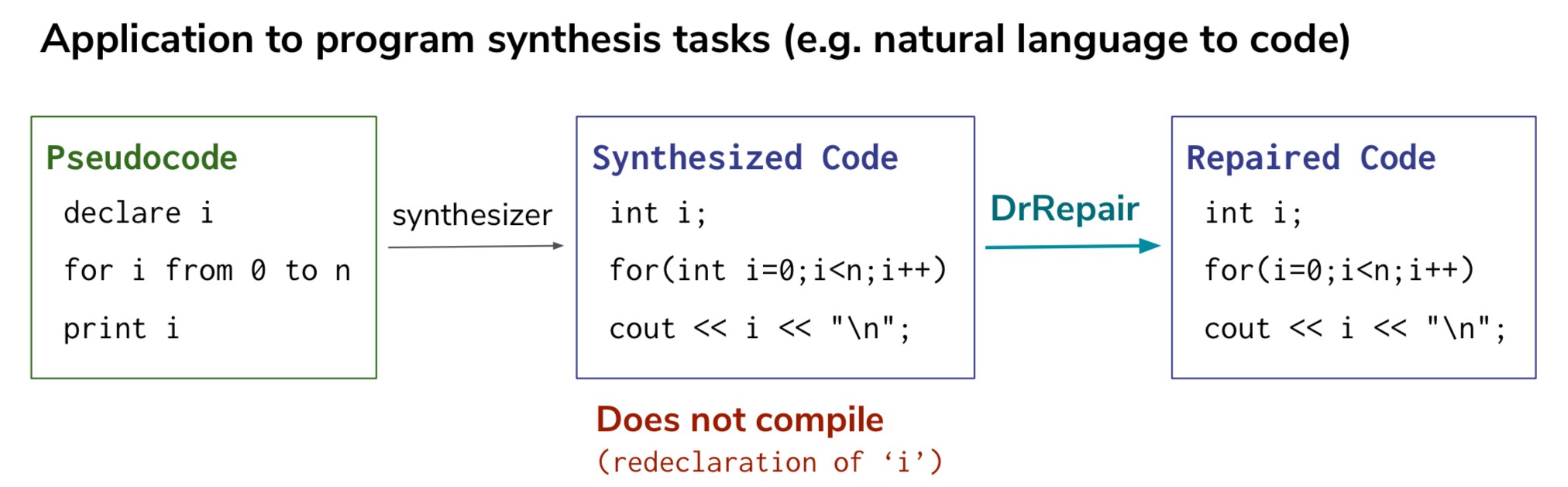
Application to SPoC (Natural Language to Code)
Program synthesis, in particular systems that can translate natural language descriptions (e.g. English) into code (e.g. Python, C++), are useful because they can help a wider range of people use programming languages. In SPoC (Pseudocode-to-Code), the task is to synthesize C++ implementation from pseudocode, a natural language description of a program. However, one challenge experienced by existing synthesizers (machine translation models applied to SPoC) is that they tend to output inconsistent code that does not compile – for instance, in the figure below, the variable i is declared twice in the synthesized code. We find that we can apply our program repair model to this invalid code and fix it into a correct one, helping the program synthesis task. In the evaluation on SPoC, the use of our repair model improves the final synthesis success rate from the existing system’s 34% to 37.6%.
Conclusion
In this work, we studied how to use machine learning to repair programs from error messages, and developed three key insights:
- Error messages provide a crucial signal for learning program repair.
- Program-feedback graphs (joint representations of code & error messages) help model the reasoning of repair (e.g. tracking variables that caused the error).
- Self-supervised learning allows us to turn freely-available, unlabeled programs (e.g. GitHub code) into useful training examples of program repair.
This work also provides a general framework of “learning from feedback”, which has various applications: editing documents based on comments, learning from users in interactive dialog, etc.
You can check out our full paper (ICML 2020) here and our source code/data on GitHub. You can also find the presentation slides on this work here. If you have questions, please feel free to email us!
- Michihiro Yasunaga: myasu@cs.stanford.edu
Acknowledgments
Many thanks to Percy Liang, as well as members of the P-Lambda lab and the Stanford NLP group for their valuable feedback, and to Sidd Karamcheti and Andrey Kurenkov for edits on this blog post!
-
Programmers’ Build Errors: A Case Study (at Google). Hyunmin Seo, Caitlin Sadowski, Sebastian Elbaum, Edward Aftandilian, Robert Bowdidge. 2014 ↩
-
Graph Attention Networks. Petar Veličković, Guillem Cucurull, Arantxa Casanova, Adriana Romero, Pietro Liò, Yoshua Bengio. 2018. ↩
-
DeepFix: Fixing common C language errors by deep learning. Rahul Gupta, Soham Pal, Aditya Kanade, Shirish Shevade. 2017. ↩
-
SPoC: Search-based Pseudocode to Code. Sumith Kulal, Panupong Pasupat, Kartik Chandra, Mina Lee, Oded Padon, Alex Aiken and Percy Liang. 2019. ↩


 Stefan Natu is a Sr. Machine Learning Specialist at AWS. He is focused on helping financial services customers build end-to-end machine learning solutions on AWS. In his spare time, he enjoys reading machine learning blogs, playing the guitar, and exploring the food scene in New York City.
 Jaipreet Singh is a Senior Software Engineer on the Amazon SageMaker Studio team. He has been working on Amazon SageMaker since its inception in 2017 and has contributed to various Project Jupyter open-source projects. In his spare time, he enjoys hiking and skiing in the Pacific Northwest.
 Huong Nguyen is a Sr. Product Manager at AWS. She is leading the user experience for SageMaker Studio. She has 13 years’ experience creating customer-obsessed and data-driven products for both enterprise and consumer spaces. In her spare time, she enjoys reading, being in nature, and spending time with her family.


 Taha A. Kass-Hout, MD, MS, is director of machine learning and chief medical officer at Amazon Web Services (AWS). Taha received his medical training at Beth Israel Deaconess Medical Center, Harvard Medical School, and during his time there, was part of the BOAT clinical trial. He holds a doctor of medicine and master’s of science (bioinformatics) from the University of Texas Health Science Center at Houston.


 Maryam Rezapoor is a Senior Product Manager with AWS AI Devices team. As a former biomedical researcher and entrepreneur, she finds her passion in working backward from customers’ needs to create new impactful solutions. Outside of work, she enjoys hiking, photography, and gardening.