Monthly Archives: February 2021

In this tutorial, we will walk through the entire machine learning (ML) life-cycle and show you how to architect and build an ML use case end to end using Amazon SageMaker. Amazon SageMaker provides a rich set of capabilities that enable data scientists, machine learning engineers, and developers to prepare, build, train, and deploy ML models rapidly and with ease. For our use case, we have chosen an automobile claims fraud detection example.

We will initially provide an architectural walkthrough of the various portions of the ML lifecycle and then point to the code that builds each section of the lifecycle on SageMaker.

To get started, data scientists use an experimental process to explore various data preparation tasks, in some cases engineering features, and eventually settle on a standard way of doing so. Then they embark on a more repeatable and scalable process of automating stages of this process, until the model provides the necessary levels of performance (such as accuracy, F1 score, and precision). Then they package this process in a repeatable, automated, and scalable ML pipeline.

The following diagram illustrates the manual investigative and the automated operational workflows.

New capabilities required for new tasks in the ML lifecycle

At a high level, the ML lifecycle looks like the following diagram.

The general phases of the ML lifecycle are data preparation, train and tune, and deploy and monitor, with inference being when we actually serve the model up with new data for inference.

As ML evolves and matures in the industry, we see an increased need for activities that support various facets of scaling of ML tasks and artifacts; making the artifacts that are the outputs of each task consistently standardized, more accessible, more transparent, and therefore more governable. In addition, each of these activities needs to scale from an exploratory activity to a consistent, automated and scalable activity via automated pipelines.

In the detailed preceding ML Lifecycle diagram, the red boxes represent comparatively newer concepts and tasks that are now deemed important to include in, and run in a scalable, operational, and production-oriented (vs. research-oriented) environment.

These newer lifecycle tasks and their corresponding Amazon SageMaker capabilities include the following:

• Data wrangling – We use SageMaker Data Wrangler for cleaning, normalizing, transforming and encoding data, as well as joining datasets. The output of SageMaker Data Wrangler is data transformation code that works with SageMaker Processing, SageMaker Pipelines, SageMaker Feature Store, or with Pandas in a plain Python script. Feature engineering can now be done faster and easier, with SageMaker Data Wrangler where we have a GUI-based environment and can generate code that can be used for the subsequent phases of the ML lifecycle.
• Detecting bias – With SageMaker Clarify, in the data prep or training phases, we can detect pre-training (data bias) and post-training bias (model bias). At the inference phase, SageMaker Clarify gives us the ability to provide interpretability and explainability of the predictions by providing insight into which factors were most influential in coming up with the prediction.
• Feature Store (offline) – After we complete our feature engineering, encoding, and transformations, we can standardize features offline in SageMaker Feature Store, to be used as input features for training models.
  SageMaker Feature Store allows you to create offline feature groups that keep all the historical data and can be used as inputs to training.
  Note that Features can be ingested from a feature processing pipeline into the online feature store and will then get replicated to the offline store. The offline store could be used to run batch inference as well. Thus, the online feature store can also be used as input for training.
• Artifact lineage: We can use SageMaker ML Lineage Tracking to associate all the artifacts (such as data, models, and parameters) with a trained model to produce metadata that is stored in a model registry. In addition, tracking human in the loop actions such as model approvals and deployments further facilitates the process of ML governance.
• Model Registry: The SageMaker Model Registry stores the metadata around all the artifacts that you include in the process of creating your models, along with the trained models themselves in a model registry. Later, we can use human approval to note that the model is ready for production. This feeds into the next phase of deploy and monitor.
• Inference and Feature Store (online): SageMaker Feature Store provides for low latency (up to single digit milliseconds) and high throughput reads for serving our model with new incoming data.
• Pipelines: After we experiment and decide on the various options in the lifecycle (such as which transforms to apply to our features, determine imbalance or bias in the data, which algorithms to choose to train with, or which hyperparameters are giving us the best performance metrics), we can automate the various tasks across the lifecycle using SageMaker Pipelines.
  This lets us streamline the otherwise cumbersome manual processes into an automated ML pipeline. To build this pipeline, we will prepare some data (customers and claims) by ingesting the data into SageMaker Data Wrangler and apply various transformations in SageMaker Data Wrangler within SageMaker Studio.  SageMaker Data Wrangler creates .flow files. We will use these transformation definitions as a starting point for our automated pipeline and go through the ML Lifecycle all the way to deploying the model to a SageMaker Hosted Endpoint. Note that some use cases may require one, larger, end-to-end pipeline, that does everything. Other use cases may require multiple pipelines, such as the following:

• • A pipeline for all data prep steps.
  • A pipeline for training, tuning, lineage, and depositing into the model registry (which we show in the code associated with this post).
  • Possibly another pipeline for specific inference scenarios (such as real time vs. batch).
  • A pipeline for triggering retraining by using SageMaker Model Monitor to detect model drift or data drift and trigger retraining using, for example, an AWS Lambda

Use case: Fraud detection for auto insurance claims

In this post, we use an auto insurance claim fraud detection use case to demonstrate how you can easily use Amazon SageMaker to predict the probability that an incoming auto claim may be fraudulent.

We dive into the implementation details in these six notebooks, where we demonstrate how you can enhance your effectiveness as a data scientist and ML engineer by using the new Amazon SageMaker services and features (pictured in red in the preceding figure) to solve problems at each stage of the ML lifecycle.

Technical solution overview

Let’s take a look at the services used in the ML lifecycle for implementing our fraud detection use case. Each section has an accompanying notebook on GitHub that you can follow as you read through the explanations in this post.

Wrangling and preprocessing the dataset

We use two synthetic datasets, consisting of customers and claims that we have synthetically generated. We use SageMaker Data Wrangler to ingest, analyze, prepare, and transform each dataset. You can do this in the GUI-based feature available in SageMaker Studio.

Second, we use SageMaker Data Wrangler to export the transformed data as two CSV files that can be picked up in an Amazon Simple Storage Service (Amazon S3) bucket by SageMaker Processing, in order to conduct scalable data preparation and preprocessing.

Storing the features

After SageMaker Processing applies the transformations defined in SageMaker Data Wrangler, we store the normalized features in an offline feature store so the features can be shared and reused consistently across an organization among collaborating data scientists. This standardization is often key to creating a normalized, reusable set of features that can be created, shared, and managed as input into training ML models. You can use this feature consistency across the ML maturity spectrum, whether you are a startup or an advanced organization with a ML Center of Excellence.

Assessing and Mitigating bias, training and tuning

The issues relating to bias detection and fairness in AI have taken a prominent role in ML. Data bias is often inadvertently injected during the data labeling and collection process, and may often be overlooked in the significance of its impact on training a model. SageMaker Clarify is a fully-managed toolkit to identify potential bias within a training dataset or model, explain individual inference results, aggregate these explanations for an entire dataset, integrate with built-in monitoring capabilities to assess production performance, and provide these capabilities across modeling frameworks.

You can use SageMaker Clarify to assess various types of bias. For example, assessing pre-training bias (data) can focus on determining if class imbalance or a variety of other factors are beyond a threshold and therefore may bias the model we seek to train. SageMaker Clarify helps improve your ML models by detecting potential biases prior to training (data bias) and after training, assess post-training bias (model bias) and can also help explain the predictions that models make during inference.

After we implement our bias mitigation strategy, the next step is often to choose a training algorithm and experiment with various ways of tuning it so as to obtain acceptable ML performance metrics such as F1, AUC, or accuracy. For this post, we use the XGBoost algorithm for training our model using the data in the feature store, and evaluate F1 metrics.

We can also check the resulting model’s post-training bias and, when satisfied with both the performance and transparency (bias) metrics, tune the model to get the most out of its performance through hyperparameter optimization.

We can track the lineage of these experiments using Lineage Tracking to track various aspects of the evolution of our experiments including answering questions related to the following:

• Data – Which dataset did we use?
• Prep – How did we clean, transform and featurize the data?
• Training – Which model and training job configuration did we use?
• Tuning – Which hyperparameters did we use?

During our experimentation, we may have trained many models, from different datasets, prepared with different transformations, each with their own performance metrics and bias metrics. If we like a result, we can look at the artifact lineage associated with it so we can reproduce those results or improve them.

Capturing artifact lineage in experiments

Not only do we want to store our trained models themselves, but also the specific datasets, feature  transformations, preprocessing mechanisms, algorithms, and hyperparameter configurations that were used to produce and optimize the models for governance and reproducibility purposes. We can store that metadata, which tracks the experiment and lineage of the model, with a reference to the data and the model in the SageMaker Model Registry.

Deploying the model to a SageMaker hosted endpoint

After we decide which models should be approved for deployment, we can deploy them to a SageMaker hosted endpoint, where they are ready for serving predictions.

Running predictions on the model using the online feature store

We create models so we can run predictions on them. We can invoke an endpoint directly, since Amazon SageMaker endpoints have load balancers behind them to balance incoming load.

Another common invocation pattern for running inference is the ML Gateway Pattern, where we expose the inference as a service endpoint and invoke it using an Amazon API Gateway. This pattern also allows the benefits of a service oriented architecture exposing a set of ML services as RESTful endpoints. Incoming service requests benefit from being load balanced, cached, and monitored using Amazon API Gateway. Amazon API Gateway then calls an AWS Lambda function which can call the SageMaker endpoint.

In this post, we will serve the endpoint by invoking it in real time using incoming data that is materialized as features in an online feature store. The resulting insurance claim is then designated as fraud or not fraud using the XGBoost trained and tuned model.

Explaining the model’s predictions

We can then inspect why this decision was made and present an explainable narrative to inquisitive parties. For this, we use the explainability features of SageMaker Clarify.

Solution architecture and ML lifecycle workflows

Let’s dive deeper and explore the solution architecture for each of the four workflows for data prep, train and tune, deploy, and finally a pipeline that ties everything together in an automated fashion up to storing the models in a registry.

Manual workflow

Before we automate parts of the lifecycle, we often conduct investigative data science work. This is often carried out in the exploratory data analysis and visualization phases, where we use SageMaker Data Wrangler to figure out what we want to do with our data (visualize, understand, clean, transform, or featurize) to prepare it for training. The following diagram illustrates the flow for the two datasets on SageMaker Data Wrangler.

One of the outputs you can choose in SageMaker Data Wrangler is a Python notebook that distills these activities into a set of functions. The .flow file output contains a set of transformations that provide SageMaker Processing with guidance on what transformations to apply to features. The following screenshot shows the export options from SageMaker Data Wrangler.

We can send this code to SageMaker Processing to create a preprocessing job that prepares our datasets for training in a scalable and reproducible way.

Data prep

The following diagram shows the data prep architecture. The code is available in the notebook 1-data-prep-e2e.ipynb.

In the attached notebook for the data prep stage, we assume all the work was done in SageMaker Data Wrangler and the output is available in the /data folder of the example code, so you can follow the flow of the notebook. You can query, explore, and visualize features using SageMaker Data Wrangler from SageMaker Studio.

You can provide an S3 bucket that contains the results of the SageMaker Data Wrangler job that has output two files: claims.csv and customer.csv. If you want to move on and assume the data prep has been conducted, you can access the preprocessed data in the /data folder containing the files claims_preprocessed.csv (31 features) and customers_preprocessed.csv (19 features). The policy_id and event_time columns in customers_preprocessed.csv are necessary when creating a feature store, which requires a unique identifier for each record and a timestamp.

Dataset features and distribution

You can find the code for exploring the data in the notebook 0-AutoClaimFraudDetection.ipynb.

Here are some sample plots that indicate the nature of the class imbalance and to what features fraud may be correlated.

The dataset is heavily weighted towards male customers.

Fraud is positively correlated with having a greater number of insurers over the past 5 years. Customers who switched insurers more frequently also had more prevalence of fraud.

We loaded the raw data from the S3 bucket and created 10 transforms for claims and 6 for customers.

Transformations and featurizations

For claims, we formatted some strings and encoded several categorical features. See the following code:

Data columns (total 31 columns):
 #   Column                           Non-Null Count  Dtype  
---  ------                           --------------  -----  
 0   policy_id                        5000 non-null   int64  
 1   incident_severity                5000 non-null   float64
 2   num_vehicles_involved            5000 non-null   int64  
 3   num_injuries                     5000 non-null   int64  
 4   num_witnesses                    5000 non-null   int64  
 5   police_report_available          5000 non-null   float64
 6   injury_claim                     5000 non-null   int64  
 7   vehicle_claim                    5000 non-null   int64  
 8   total_claim_amount               5000 non-null   int64  
 9   incident_month                   5000 non-null   int64  
 10  incident_day                     5000 non-null   int64  
 11  incident_dow                     5000 non-null   int64  
 12  incident_hour                    5000 non-null   int64  
 13  fraud                            5000 non-null   int64  
 14  driver_relationship_self         5000 non-null   float64
 15  driver_relationship_na           5000 non-null   float64
 16  driver_relationship_spouse       5000 non-null   float64
 17  driver_relationship_child        5000 non-null   float64
 18  driver_relationship_other        5000 non-null   float64
 19  incident_type_collision          5000 non-null   float64
 20  incident_type_breakin            5000 non-null   float64
 21  incident_type_theft              5000 non-null   float64
 22  collision_type_front             5000 non-null   float64
 23  collision_type_rear              5000 non-null   float64
 24  collision_type_side              5000 non-null   float64
 25  collision_type_na                5000 non-null   float64
 26  authorities_contacted_police     5000 non-null   float64
 27  authorities_contacted_none       5000 non-null   float64
 28  authorities_contacted_fire       5000 non-null   float64
 29  authorities_contacted_ambulance  5000 non-null   float64
 30  event_time                       5000 non-null   float64

For customers, we have the following code:

#   Column                     Non-Null Count  Dtype  
---  ------                     --------------  -----  
 0   policy_id                  5000 non-null   int64  
 1   customer_age               5000 non-null   int64  
 2   customer_education         5000 non-null   int64  
 3   months_as_customer         5000 non-null   int64  
 4   policy_deductable          5000 non-null   int64  
 5   policy_annual_premium      5000 non-null   int64  
 6   policy_liability           5000 non-null   int64  
 7   auto_year                  5000 non-null   int64  
 8   num_claims_past_year       5000 non-null   int64  
 9   num_insurers_past_5_years  5000 non-null   int64  
 10  customer_gender_male       5000 non-null   float64
 11  customer_gender_female     5000 non-null   float64
 12  policy_state_ca            5000 non-null   float64
 13  policy_state_wa            5000 non-null   float64
 14  policy_state_az            5000 non-null   float64
 15  policy_state_or            5000 non-null   float64
 16  policy_state_nv            5000 non-null   float64
 17  policy_state_id            5000 non-null   float64
 18  event_time                 5000 non-null   float64

Preprocessing

Data is exported from SageMaker Data Wrangler into an S3 bucket. It’s then preprocessed using SageMaker Processing. We assume that the output of the preprocessing job has been deposited in the S3 bucket you provide, or you can find the preprocessed data in the /data folder.

Ingesting the preprocessed data into SageMaker Feature Store

After SageMaker Processing finishes the preprocessing and we have our two CSV data files for claims and customers ready. We have contributed to the standardization of these features by making them discoverable and reusable by ingesting them into SageMaker Feature Store.

SageMaker Feature Store is a centralized store for features and their associated metadata, allowing features to be easily discovered and reused across your organization or team. You have the option of creating an offline feature store (stored in Amazon S3) or an online component stored in a low-latency store, or both. Data is stored in your S3 bucket using a prefixing scheme based on event time. The offline feature store is append-only, which enables you to maintain a historical record of all feature values. Data is stored in the offline store in Parquet format for optimized storage and query access. SageMaker Feature Store supports combining data to produce, train, validate, and test datasets, and allows you to extract data at different points in time.

To store features, we first need to define their feature group. A feature group is the main feature store resource that contains the metadata for all the data stored in Amazon SageMaker Feature Store. A feature group is a logical grouping of features, defined in the feature store, to describe records. A feature group’s definition is composed of a list of feature definitions, a record identifier name, and configurations for its online and offline store.

The online database is optional, but very useful if you need supplemental features to be available at inference. In this section, we create two feature groups for our claims and customers datasets. After inserting the claims and customers data into their respective feature groups, you need to query the offline store with Amazon Athena to build the training dataset.

To ingest data, we first designate a feature group for each type of feature, in this case, one per CSV file. You can ingest data into feature groups in SageMaker Feature Store in one of two ways: streaming or batch. For this post, we use the batch method.

When the offline feature store is ready, a crawler catalogs it and loads the catalog into an Athena table. To construct the train and test datasets, we use a SQL query to join the claims and customers tables that were created in Athena.

Training and tuning

The code for this section can be found in the following notebooks: 2-lineage-train-assess-bias-tune-registry-e2e.ipynb and 3-mitigate-bias-train-model2-registry-e2e.ipynb. The following diagram illustrates the workflow for the bias check, training, tuning, lineage, and model registry stages.

We write the train and test split datasets to our designated S3 bucket, and create an XGBoost estimator to train our fraud detection model with a fraud or no fraud logistic target. Prior to starting the SageMaker training job using the built-in XGBoost algorithm, we set the XGBoost hyperparameters. You can learn more about XGBoost’s Learning Task Parameters, Tree Booster Parameters.

We take the opportunity to track all the artifacts or entities involved with the training job so we can track the lineage of the model. This is done by importing several sagemaker.lineage components. See the following code:

from sagemaker.lineage import context, artifact, association, action.

Lineage Tracking provides us with visibility into the code, training data,  and model artifacts that we then associate with association_type='Produced' and association_type='ContributesTo', which links what contributed to and what produced a given artifact in the process.

We also assess degrees of pre-training and post-training bias using SageMaker Clarify. Pre-training metrics show a variety of possible preexisting bias in our dataset. Post-training metrics show bias in the predictions resulting from the model. We use analysis_config.json to specify which groups we want to check bias across and which metrics we want to show.

We assess two metrics: the difference in positive proportions in predicted labels (DPPL) and if a class imbalance exists in the data. For our use case, we measure this on the gender feature, which indicates if we have more male customers than female customers. Results indicate a slight bias in our model measured by the DPPL metric.

Deploying and serving the model

The code for this section can be found in the notebook 4-deploy-run-inference-e2e.ipynb. The following diagram shows the deploy and serve stage for real-time inference.

We choose the model that conforms to our metrics best, with an appropriate tolerance of F1 score, and deploy that model by creating a SageMaker training job that results in deploying the model to a SageMaker hosted endpoint.

When the endpoint is in place, we use the online feature store to run inference on the endpoint.

Interpreting the results

The following plot shows the data features and their relative impact on the prediction, using SHAP values.

We can trace back much of our interpretation of inference results to the features that had the most impact on the model output.

Creating an automated workflow using SageMaker Pipelines

The code for this section can be found in the notebook 5-pipeline-e2e.ipynb.

After we complete a few iterations of our manual exploratory data science and are happy with the outcomes of our cleansing, transformations, and featurizations, we may want to create an automated workflow using SageMaker Pipelines, so we can scale and don’t have to go through this manual process every time.

The following diagram shows our end-to-end automated MLOps pipeline, which includes eight steps:

1. Preprocess the claims data with SageMaker Data Wrangler.
2. Preprocess the customers data with SageMaker Data Wrangler.
3. Create a dataset and train/test split.
4. Train the XGBoost algorithm.
5. Create the model.
6. Run bias metrics with SageMaker Clarify.
7. Register the model.
8. Deploy the model.

Conclusion

In December 2020, AWS announced many new AI and ML services and features. In this post, we discussed how to build an end to end fraud detection use case for auto insurance claims using most of the these new capabilities including: SageMaker Data Wrangler for feature transformation, SageMaker Processing for preprocessing data, SageMaker Feature Store (offline) for standardization of features, SageMaker Clarify for bias detection pre- and post-training and for post-inference interpretability of results, ML Lineage Tracking to help with governance of ML artifacts, SageMaker Model Registry for model and metadata storage, and SageMaker Pipelines for end to end workflow automation. Additional information about each of these services can be found by checking out the following product page links.

• Amazon SageMaker Data Wrangler
• Amazon SageMaker Feature Store
• Amazon SageMaker Clarify
• Amazon SageMaker Pipelines

About the Author

Dr. Ali Arsanjani is the Tech Sector AI/ML Leader and Principal Architect for AI/ML Specialist Solution Architects with AWS helping customers make optimal use of ML using the AWS platform. He is also an adjunct faculty member at San Jose State University, teaching and advising students in the Data Science Masters Programs.

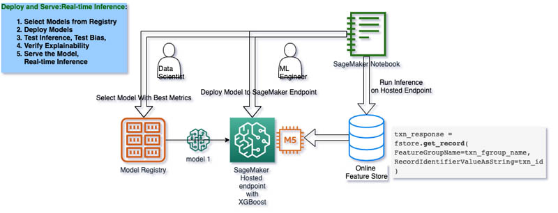
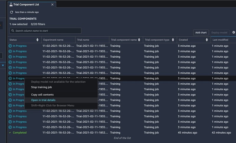
Read More

Each year, organizations lose tens of billions of dollars to online fraud globally. Organizations such as ecommerce companies and credit card companies use machine learning (ML) to detect online fraud. Some of the most common types of online fraud include email account compromise (personal or business), new account fraud, and non-payment or non-delivery (including card numbers compromised).

A common challenge with ML is the need for a large labeled dataset to create ML models for detecting fraud. Moreover, even if you have this dataset, you need the skill set and infrastructure to build, train, deploy, and scale your ML model to detect fraud with millions of events. In addition, you need humans to review the subset of high-risk fraud predictions to ensure that the results are highly accurate. Setting up a human review system with your fraud detection model requires provisioning complex workflows and managing a group of reviewers, which increases the time to market for your applications and overall costs.

In this post, we provide an approach to identify high-risk predictions from Amazon Fraud Detector and use Amazon Augmented AI (Amazon A2I) to set up a human review workflow to automatically trigger a review process for further investigation and validation.

Amazon Fraud Detector is a fully managed service that uses ML and more than 20 years of fraud detection expertise from Amazon to identify potential fraudulent activity so you can catch more online fraud faster. Amazon Fraud Detector automates the time-consuming and expensive steps to build, train, and deploy an ML model for fraud detection, making it easier for you to leverage the technology. Amazon Fraud Detector customizes each model it creates to your dataset, making the accuracy of models higher than current one-size-fits-all ML solutions. And because you pay only for what you use, you avoid large upfront expenses.

Amazon A2I is an ML service that makes it easy to build the workflows with ML models required for human review. Amazon A2I brings human review to all developers, removing the undifferentiated heavy lifting associated with building human review systems or managing large numbers of reviewers.

Overview of the solution

The high-level solution is summarized through the following architecture.

The workflow contains the following steps:

1. The client application sends information to the Amazon Fraud Detector endpoint.
2. Amazon Fraud Detector predicts a risk score (in the range of 0–1,000) on the input data with an ML model that is trained using historical data. A score of 0 indicates that the prediction is considered to have the lowest possible risk, and a score of 1,000 indicates that the prediction is considered to have the highest possible risk.
3. If the risk score for a particular prediction falls beneath a predefined threshold, there is no further action.
4. If the risk score exceeds the predefined threshold (for example, a score of 900), the Amazon A2I loop starts automatically and sends predictions for human review to an Amazon A2I private workforce. A private workforce can be employees of your company. They open the Amazon A2I interface, review the case, and make an adjudication (approve, deny, or send it for further verification).
5. The approval or rejection result from the private workforce is stored in Amazon Simple Storage Service (Amazon S3). From Amazon S3, it can be directly sent to the client application.

Solution walkthrough

In this post, we set up Amazon Fraud Detector using the AWS Management Console, and set up Amazon A2I using an Amazon SageMaker notebook. The following steps outline the detailed solution:

1. Train and deploy the Amazon Fraud Detector model using historical data.
2. Set up an Amazon A2I human loop with Amazon Fraud Detector.
3. Use the model to predict the risk score for a given new input data.
4. Set up an Amazon A2I human workflow and loop.

Prerequisites

Before getting started, you must complete the following prerequisite steps:

1. Download the training data. For this post, we use synthetic training data.
2. Create an S3 bucket named fraud-detector-a2i and upload the training data to the bucket.

Training and deploying the Amazon Fraud Detector model

This section covers the high-level steps for building the model and creating a fraud detector:

1. Create an event to evaluate for fraud.
2. Define the model and training details to train the model using the data previously uploaded to Amazon S3.
3. Deploy the model.
4. Create the detector. 

Creating an event

Navigate to the Amazon Fraud Detector console. You uploaded the training dataset to Amazon S3 in the prerequisite steps. In this step, we create an event. An event is a business activity that is evaluated for fraud risk, and the event type defines the structure for an event sent to Amazon Fraud Detector.

1. On the Amazon Fraud Detector console, choose Create event.
2. For Name, enter registration.
3. For Entity, choose Create new entity.

The entity represents who is performing or triggering the event.

4. For Entity type name, enter customer.

5. For Choose how to define this event’s variables, choose Select variables from a training dataset.
6. For AWS Identity and Access Management or IAM role, choose Create IAM role.

7. In the Create IAM role section, enter the specific bucket name where you uploaded your training data. 

The name of IAM role should be the S3 bucket name where you uploaded your training data. Otherwise, you get an Access denied Exception error.

8. Choose Create role.

9. For Data location, enter the path to your training data.
10. Choose Upload.

This pulls in the variables from the previously uploaded dataset. Choose the variable types as shown in the following screenshot.

You need to create at least two labels for the model to use.

11. For Labels, choose fraud and legit.

12. Choose Create event type.

Creating the model

When the event is successfully created, move on to create the model.

1. On the Define model details page, for Model name¸ enter sample_fraud_detection.
2. For Model type, choose Online Fraud Insights.
3. For Event type, choose registration.
4. For IAM role, choose the role you created earlier or create a new one.
5. For Training data location, enter the path to your training data; for example, s3://<bucket-name>/<object name>.
6. Choose Next.

7. On the Configure training page, for Model inputs, select all the variables from your historical event dataset.
8. For Fraud labels, choose fraud.
9. For Legitimate labels, choose legit.
10. Choose Next.

11. Choose Create and train model.

The process of creating and training the model takes approximately 45 minutes to complete. When the model has stopped training, you can check model performance by choosing the model version. 

Amazon Fraud Detector validates model performance using 15% of your data that was not used to train the model and provides performance metrics, including the confusion matrix and the area under the curve (AUC). You need to consider these metrics together with your business objectives (minimize false positives). For further details on the metrics and how to determine thresholds, see Fraud Detector Training performance metrics.

The following screenshot shows our model performance.

Deploying the model

When the model is trained, you’re ready to deploy it.

1. Choose your model (sample_fraud_detection) and the version you want to deploy.
2. On the model version details page, on the Actions menu, choose Deploy model version.

Creating a detector

After you deploy your model, you need to create a detector to hold your deployed model and decision logic.

1. On the Amazon Fraud Detector console, choose Detectors.
2. Choose Create detector.
3. For Detector name, enter fraud_detector.
4. For Event type, choose registration.
5. Choose Next.

5. In the Add model section, for Model, choose your model and its version.

6. Choose Next.

You need to create rules to interpret what is considered a high-risk event based on the model score produced by your detector.

7. In the Add rules section, for Name, enter high_fraud_risk.
8. For Expression, enter the following code:

   $ sample_fraud_detection_insightscore > 900,

Each rule must contain a single expression that captures your business logic. All expressions must evaluate to a Boolean value (true or false) and be less than 4,000 characters in length. If-else type conditions are not supported. All variables used in the expression must be predefined in the evaluated event type. For help with more advanced expressions, see Rule language reference.

9. For Outcomes, choose the outcome you want for your rule.

An outcome is the result of a fraud prediction. Create an outcome for each possible fraud prediction result. For example, you may want outcomes to represent risk levels (high_risk, medium_risk, and low_risk) or actions (approve, review). You can add one or more outcomes to a rule.

10. Choose Add rule to run the rule validation checker and save the rule.

11. In the Configure rule execution section, for Rule execution modes, select First matched.
12. Choose Next.

13. In the Review and Create section, choose Create detector.

We have successfully created the detector.

Setting up an Amazon A2I human loop with Amazon Fraud Detector

In this section, we show you to configure an Amazon A2I custom task type with Amazon Fraud Detector using the accompanying Jupyter notebook. We use a custom task type to integrate a human review loop into any ML workflow. You can use a custom task type to integrate Amazon A2I with other AWS services like Amazon Comprehend, Amazon Transcribe, and Amazon Translate, as well as your own custom ML workflows.

To get started, complete the following steps:

1. Create a notebook instance in SageMaker.

Make sure your SageMaker notebook has AWS Identity and Access Management (IAM) roles and permissions for FraudDetectorFullAccess and SagemakerFullAccess, and Amazon S3 read and write access to the bucket you specified in BUCKET.

2. When the notebook is active, choose Open Jupyter.
3. On the Jupyter dashboard, choose New, and choose
4. In the terminal, enter the following code:

   cd SageMaker; 
   git clone https://github.com/aws-samples/amazon-a2i-sample-jupyter-notebooks

5. Open the notebook by choosing Amazon A2I and Amazon Fraud Detector.ipynb in the root folder.
6. Run the Install and Setup steps to install the necessary libraries.
7. To set up the S3 bucket in the notebook, enter the bucket you created in the prerequisite step in which you uploaded your training data:

   # Replace the following with your bucket name
   BUCKET = ' fraud-detector-a2i '

8. Run the next cells to assert your bucket is in same Region in which you’re running this notebook.

For this post, you create a private work team and add only one user (you) to it.

9. On the SageMaker console, create a private workforce.
10. After you create the private workforce, find the workforce ARN and enter the ARN in the notebook:

    WORKTEAM_ARN = "your workteam arn"

11. Run the notebook cells to complete setting up, such as initializing Amazon Fraud Detector Python Boto3 APIs.
12. After you create your fraud detector model, replace the MODEL_NAME, DETECTOR_NAME, EVENT_TYPE, and ENTITY_TYPE with your model values:

    MODEL_NAME = 'sample_fraud_detection'
    DETECTOR_NAME = 'fraud_detector'
    EVENT_TYPE = 'registration'
    ENTITY_TYPE = 'customer'
    

Testing the fraud detector with a sample data record

Run the Amazon Fraud Detector Get Event Prediction API on sample data. This API provides a model score on the event and an outcome based on the designated detector. See the following code:

eventId = uuid.uuid1()
timestampStr = '2013-07-16T19:00:00Z'

# Construct a sample data record

rec = {
   'ip_address': '36.72.99.64',
   'email_address': 'fake_bakermichael@example.net',
   'billing_state' : 'NJ',
   'user_agent' : 'Mozilla',
   'billing_postal' : '32067',
   'phone_number' :'555-555-0100',
   'user_agent' : 'Mozilla',
   'billing_address' :'12351 Amanda Knolls Fake St'
}


pred = client.get_event_prediction(detectorId=DETECTOR_NAME, 
                                   detectorVersionId='1',
                                   eventId = str(eventId),
                                   eventTypeName = EVENT_TYPE,
                                   eventTimestamp = timestampStr, 
                                   entities = [{'entityType': ENTITY_TYPE, 'entityId':str(eventId.int)}],
                                   eventVariables=rec)

The API provides the following output:

pred
{'modelScores': [{'modelVersion': {'modelId': 'sample_fraud_detection',
    'modelType': 'ONLINE_FRAUD_INSIGHTS',
    'modelVersionNumber': '1.0'},
   'scores': {'sample_fraud_detection_insightscore': 992.0}}],
 'ruleResults': [{'ruleId': 'high-risk', 'outcomes': ['verify']}],
 'ResponseMetadata': {'RequestId': '8902a475-df5b-470d-a990-ec217d5908cd',
  'HTTPStatusCode': 200,
  'HTTPHeaders': {'date': 'Mon, 02 Nov 2020 17:22:11 GMT',
   'content-type': 'application/x-amz-json-1.1',
   'content-length': '250',
   'connection': 'keep-alive',
   'x-amzn-requestid': '8902a475-df5b-470d-a990-ec217d5908cd'},
  'RetryAttempts': 0}}

Run the following notebook cell to print the model score:

pred['modelScores'][0]['scores']['sample_fraud_detection_insightscore']

Creating a human task UI using a custom worker task template

Use HTML elements to create a custom worker template that Amazon A2I uses to generate your worker task UI. For instructions on creating a custom template, see Create Custom Worker Task Template. We have over 70 pre-built UIs or worker task templates for various use cases. For this post, we use the following custom task template to flag the high-risk output as Fraudulent, Valid, or Needs further Investigation:

template="""<script src="https://assets.crowd.aws/crowd-html-elements.js"></script>

<crowd-form>
      <crowd-classifier
          name="category"
          categories="['Fradulent, 'Valid, 'Needs further Review]"
          header="Select the most relevant category"
      >
      <classification-target>
        <h3><strong>Risk Score (out of 1000): </strong><span style="color: #ff9900;">{{ task.input.score.sample_fraud_detection_insightscore }}</span></h3>
        <hr>
        <h3> Claim Details </h3>
        <p style="padding-left: 50px;"><strong>Email Address   :  </strong>{{ task.input.taskObject.email_address }}</p>
        <p style="padding-left: 50px;"><strong>Billing Address :  </strong>{{ task.input.taskObject.billing_address }}</p>
        <p style="padding-left: 50px;"><strong>Billing State   :  </strong>{{ task.input.taskObject.billing_state }}</p>
        <p style="padding-left: 50px;"><strong>Billing Zip     :  </strong>{{ task.input.taskObject.billing_postal }}</p>
        <p style="padding-left: 50px;"><strong>Originating IP  :  </strong>{{ task.input.taskObject.ip_address }}</p>
        <p style="padding-left: 50px;"><strong>Phone Number    :  </strong>{{ task.input.taskObject.phone_number }}</p>
        <p style="padding-left: 50px;"><strong>User Agent      :  </strong>{{ task.input.taskObject.user_agent }}</p>
      </classification-target>
      
      <full-instructions header="Claim Verification instructions">
      <ol>
        <li><strong>Review</strong> the claim application and documents carefully.</li>
        <li>Mark the claim as valid or fraudulent</li>
      </ol>
      </full-instructions>

      <short-instructions>
           Choose the most relevant category that is expressed by the text. 
      </short-instructions>
    </crowd-classifier>

</crowd-form>
"""

You can create a worker task template using the SageMaker console and the SageMaker API operation CreateHumanTaskUi. Run the following cell to create the human task UI for fraud detection:

def create_task_ui(task_ui_name, template):
    '''
    Creates a Human Task UI resource.

    Returns:
    struct: HumanTaskUiArn
    '''
    response = sagemaker.create_human_task_ui(
        HumanTaskUiName=task_ui_name,
        UiTemplate={'Content': template})
    return response
taskUIName = 'fraud'+ str(uuid.uuid1())

# Create task UI
humanTaskUiResponse = create_task_ui(taskUIName, template)
humanTaskUiArn = humanTaskUiResponse['HumanTaskUiArn']
print(humanTaskUiArn)

Creating a human review workflow definition

Workflow definitions allow you to specify the following:

• The worker template or human task UI you created in the previous step.
• The workforce that your tasks are sent to. For this post, it’s the private workforce you created in the prerequisite steps.
• The instructions that your workforce receives.

This post uses the Create Flow Definition API to create a workflow definition. Run the following cell in the notebook:

def create_flow_definition(flow_definition_name):
    '''
    Creates a Flow Definition resource

    Returns:
    struct: FlowDefinitionArn
    '''
    response = sagemaker.create_flow_definition(
            FlowDefinitionName= flow_definition_name,
            RoleArn= ROLE,
            HumanLoopConfig= {
                "WorkteamArn": WORKTEAM_ARN,
                "HumanTaskUiArn": humanTaskUiArn,
                "TaskCount": 1,
                "TaskDescription": "Please review the  data and flag for potential fraud",
                "TaskTitle": " Review and Approve / Reject Amazon Fraud detector predictions. "
            },
            OutputConfig={
                "S3OutputPath" : OUTPUT_PATH
            }
        )
    
    return response['FlowDefinitionArn']

Optionally, you can create this workflow definition on the Amazon A2I console. For instructions, see Create a Human Review Workflow.

Setting threshold to start a human loop for high-risk scores from Amazon Fraud Detector predictions

As outlined earlier, you can invoke the Amazon Fraud Detector model endpoint to detect the risk score for given input data. If the risk score is greater than a certain threshold (for example, 900), you create and start the Amazon A2I human loop.

You can change the value of the SCORE_THRESHOLD depending on the risk level for triggering the human review. pred refers to the prediction from the sample record rec from the earlier code. Run the following cell to set up your threshold:

FraudScore= pred['modelScores'][0]['scores']['sample_fraud_detection_insightscore']
print(FraudScore)

SCORE_THRESHOLD = 900
if FraudScore > SCORE_THRESHOLD :

    # Create the human loop input JSON object
    humanLoopInput = {
        'score' : pred['modelScores'][0]['scores'],
        'taskObject': rec
    }

print(json.dumps(humanLoopInput))

Below is the response:

996.0
{"score": {"sample_fraud_detection_insightscore": 996.0}, "taskObject": {"ip_address": "36.72.99.64", "email_address": "fake_bakermichael@example.net", "billing_state": "NJ", "user_agent": "Mozilla", "billing_postal": "32067", "phone_number": "'555-555-0100", "billing_address": "12351 Amanda Knolls Fake St"}}

Starting a human loop for high risk Amazon Fraud detector’s predictions

We send the human loop input for human review and start the Amazon A2I loop with the start-human-loop API. When using Amazon A2I for a custom task, a human loop starts when StartHumanLoop is called in your application. Run the following cell in the notebook to start the human loop:

# Create flow definition
uniqueId = str(int(round(time.time() * 1000)))
flowDefinitionName = f'fraud-detector-a2i-{uniqueId}'
flowDefinitionArn = create_flow_definition(flowDefinitionName)

# Start the human loop
humanLoopName = 'Fraud-detector-' + str(int(round(time.time() * 1000)))
print('Starting human loop - ' + humanLoopName)

response = a2i_runtime_client.start_human_loop(
                            HumanLoopName=humanLoopName,
                            FlowDefinitionArn= flowDefinitionArn,
                            HumanLoopInput={
                                'InputContent': json.dumps(humanLoopInput)
                                }
                            )

Checking the status of the human loop

Run the following accompanying notebook cell to get a login link to navigate to the private workforce portal:

workteamName = WORKTEAM_ARN[WORKTEAM_ARN.rfind('/') + 1:]
print("Navigate to the private worker portal and do the tasks. Make sure you've invited yourself to your workteam!")
print('https://' + sagemaker.describe_workteam(WorkteamName=workteamName)['Workteam']['SubDomain'])

Use the generated link to log in to the private worker portal. Choose Start working to review the results.

On the next page, you can review and classify the fraud detector’s response or send it for further reviews.

The private worker can review the results and submit a response by selecting an option, for example Needs further review and choose Submit.

Evaluating the results

When the labeling work is complete for each high-risk prediction, your results should be available in the S3 output path specified in the human review workflow definition. The human answers (labels) are returned and saved in a JSON file. Run the notebook cell to get the results from Amazon S3:

import re
import pprint
pp = pprint.PrettyPrinter(indent=2)

def retrieve_a2i_results_from_output_s3_uri(bucket, a2i_s3_output_uri):
    '''
    Gets the json file published by A2I and returns a deserialized object
    '''
    splitted_string = re.split('s3://' +  bucket + '/', a2i_s3_output_uri)
    output_bucket_key = splitted_string[1]

    response = s3.get_object(Bucket=bucket, Key=output_bucket_key)
    content = response["Body"].read()
    return json.loads(content)
    

for human_loop_name in completed_loops:

    describe_human_loop_response = a2i_runtime_client.describe_human_loop(
        HumanLoopName=human_loop_name
    )
    
    print(f'nHuman Loop Name: {describe_human_loop_response["HumanLoopName"]}')
    print(f'Human Loop Status: {describe_human_loop_response["HumanLoopStatus"]}')
    print(f'Human Loop Output Location: : {describe_human_loop_response["HumanLoopOutput"]["OutputS3Uri"]} n')
    
    # Uncomment below line to print out a2i human answers
    pp.pprint(retrieve_a2i_results_from_output_s3_uri(BUCKET, describe_human_loop_response['HumanLoopOutput']['OutputS3Uri']))

The following code is the human reviewed output with labels you just submitted:

Human Loop Name: Fraud-detector-1613589638354
Human Loop Status: Completed
Human Loop Output Location: : s3://a2i-fd-demos-2020/a2i-results/fraud-detector-a2i-1613589635065/2021/02/17/19/20/38/Fraud-detector-1613589638354/output.json 

{ 'flowDefinitionArn': 'arn:aws:sagemaker:us-east-1:534095625703:flow-definition/fraud-detector-a2i-1613589635065',
  'humanAnswers': [ { 'acceptanceTime': '2021-02-17T19:20:52.563Z',
                      'answerContent': { 'category': { 'label': 'Needs furthur '
                                                                'review'}},
                      'submissionTime': '2021-02-17T19:23:38.092Z',
                      'timeSpentInSeconds': 165.529,
                      'workerId': '7fe4cd6b55282093',
                      'workerMetadata': { 'identityData': { 'identityProviderType': 'Cognito',
                                                            'issuer': 'https://cognito-idp.us-east-1.amazonaws.com/us-east-1_1DCLqiVmd',
                                                            'sub': 'ec69f8cb-3505-4fef-a2d7-56d1b974644a'}}}],
  'humanLoopName': 'Fraud-detector-1613589638354',
  'inputContent': { 'score': {'sample_fraud_detection_insightscore': 996},
                    'taskObject': { 'billing_address': '12351 Amanda Knolls '
                                                       'Fake St',
                                    'billing_postal': '32067',
                                    'billing_state': 'NJ',
                                    'email_address': 'fake_bakermichael@example.net',
                                    'ip_address': '36.72.99.64',
                                    'phone_number': '555-555-0100',
                                    'user_agent': 'Mozilla'}}}

To improve model performance of the existing Amazon Fraud Detector model, you can combine the preceding JSON response from Amazon A2I with your existing training dataset and retrain your model with a new version.

Cleaning up

To avoid incurring unnecessary charges, delete the resources used in this walkthrough when not in use. For instructions, see the following:

• How do I delete an S3 Bucket?
• Delete a Flow Definition
• Cleanup: SageMaker Resources
• Delete Fraud Detector

Conclusion

This post demonstrated how you can detect online fraud using Amazon Fraud Detector and set up human review workflows using Amazon A2I custom task type to review and validate high-risk predictions. If this post helps you or inspires you to solve a problem, we would love to hear about it! The code for this solution is available on the GitHub repo for you to use and extend. Contributions are always welcome!

About the Authors

Srinath Godavarthi is a Senior Solutions Architect at AWS and is based in the Washington, DC, area. In that role, he helps public sector customers achieve their mission objectives with well-architected solutions on AWS. Prior to AWS, he worked with various systems integrators in healthcare, public safety, and telecom verticals. He focuses on innovative solutions using AI and ML technologies.

Mona Mona is an AI/ML Specialist Solutions Architect based out of Arlington, VA. She works with the World Wide Public Sector team and helps customers adopt machine learning on a large scale. She is passionate about NLP and ML explainability areas in AI/ML. Prior to AWS, she did her masters in Computer Information Systems with a major in Big Data Analytics, and has worked for various IT consultants in the global markets domain.

Pranusha Manchala is a Solutions Architect at AWS based in Virginia. She works with hundreds of EdTech customers and provides them with architectural guidance for building highly scalable and cost-optimized applications on AWS. She found her interests in machine learning and artificial intelligence and started to dive deep into this technology. Prior to AWS, she did her masters in Computer Science with double majors in Networking and Cloud Computing.

Read More

This post is co-authored by Jiahang Zhong, Head of Data Science at Zopa. 

Zopa is a UK-based digital bank and peer to peer (P2P) lender. In 2005, Zopa launched the first ever P2P lending company to give people access to simpler, better-value loans and investments. In 2020, Zopa received a full bank license to offer people more ways to feel good about money. Since 2005, it has lent out over £5 billion to almost half a million borrowers and generated over £250 million in interest for investors on the platform. Zopa’s key business objectives are to identify quality borrowers, offer competitive credit products to them, and provide great customer experience. Technology and machine learning (ML) are at the core of their business, with applications ranging from credit risk modeling to fraud detection and customer service.

In this post, we use Zopa’s fraud detection system for loans to showcase how Amazon SageMaker Clarify can explain your ML models and improve your operational efficiency.

Business context

Every day, Zopa receives thousands of loan applications and lends out millions of pounds to their borrowers. Due to the nature of its products, Zopa is also a target for identity fraudsters. To combat this, Zopa uses advanced ML models to flag suspicious applications for human review, while leaving the majority of genuine applications to be approved by the highly automated system.

Although a primary objective of such models is to achieve great classification performance, another important concern at Zopa is the explainability of these models, for the following reasons:

• As a financial service provider, Zopa is obligated to treat customers fairly and provide reasonable visibility into its automated decisions.
• The data scientists at Zopa need to demonstrate the validity of the model and understand the impact of each input feature.
• The manual review by the underwriters can be quicker if they know why the model has considered a case as suspicious. They can also be more focused in their investigations and reduce friction in the customer experience.

Technical challenge

The advanced ML algorithms used in Zopa’s fraud detector can learn the non-linear relationship and interactions between the input features. Instead of a constant proportional effect, an input feature can have different levels of impact on each model prediction.

The data scientists at Zopa often used several traditional feature importance methods to understand the impact of the input features in non-linear ML models, such as the Partial Dependence Plots and Permutation Feature Importance. However, these methods can only provide summary insights about the model for a specific population. For the purposes we described, Zopa needed to explain the contribution of each input feature into an individual model score. SHAP (SHapley Additive exPlanations), based on the concept of a Shapley value from the field of cooperative game theory, works well for such a scenario.

There are multiple explainability techniques for individual inference to choose from, each with their pros and cons. For example, Tree SHAP is only applicable to tree-based models, and Integrated Gradients are specific to deep learning models. LIME is model agnostic but not always robust, and Kernel SHAP is computationally expensive. Because Zopa uses an ensemble of models, including gradient boosted trees and neural networks, the choice of specific explainability technique needs to accommodate the range of models used.

As a contrastive explainability technique, SHAP values are calculated by evaluating the model on synthetic data generated against a baseline sample. The explanations of the same case can be different depending on the choices of this baseline sample. This can be partly due to the distinct distributions of the chosen baseline population, such as their demographics. It can also be mere statistical fluctuation due to the limited size of the baseline sample constrained by the computation expense. Therefore, it’s important for the data scientists at Zopa to try out various choices of baseline samples efficiently.

After the SHAP explanations are produced at the granularity of an individual inference, the data scientists at Zopa also want to have an aggregated view over a certain inference population to understand the overall impact. This allows them to spot common patterns and outliers and adjust the model accordingly.

Why SageMaker Clarify

SageMaker is a fully managed service to prepare, build, train, and deploy high-quality ML models quickly by bringing together a broad set of capabilities purpose-built for ML. SageMaker Clarify provides ML developers with greater visibility into your training data and models so you can identify and limit bias, and explain predictions.

One of the key factors why Zopa chose SageMaker Clarify was due to the benefit of a fully managed service for model explanations with pay-as-you-go billing and the integration with the training and deployment phases of SageMaker.

Zopa trains its fraud detection model on SageMaker and can use SageMaker Clarify to view a feature attributions plot in SageMaker Experiments after the model has been trained. These details may be useful for compliance requirements or can help determine if a particular feature has more influence than it should on overall model behavior.

In addition, SageMaker Clarify uses a scalable and efficient implementation of Kernel SHAP, resulting in performance efficiency and cost savings for Zopa that would be incurred if it managed its own compute resources using the open-source algorithm.

Also, Kernel SHAP is model agnostic, and Clarify supports efficient processing of models with multiple outcomes via Spark-based parallelization. This is important to Zopa because it typically uses a combination of different frameworks like XGBoost and TensorFlow, and requires explainability for each model outcome. SHAP values of individual predictions can be computed via a SageMaker Clarify processing job and made available to the underwriting team to understand individual predictions.

SHAP explanations are contrastive and account for deviations from a baseline. Different baselines can generate different explanations, and SageMaker Clarify allows you to input a baseline of your choice. A non-informative baseline can be constructed as the average or random instance from the training dataset, or an informative baseline can be constructed by setting the non-actionable features to the same value as in the given instance. For more information about baseline choices and settings, see SHAP Baselines for Explainability.

Solution overview

Zopa’s fraud detection models use a few dozen input features, such as application details, device information, interaction behavior, and demographics. For model building, the training dataset was extracted from their Amazon Redshift data warehouse and cleaned up before being stored into Amazon Simple Storage Service (Amazon S3). Because Zopa has its own in-house ML library for both feature engineering and ML framework support, it uses the bring your own container (BYOC) approach to leverage the SageMaker managed services and advanced functionalities such as hyperparameter optimization. The optimized models are then deployed through a Jenkins CI/CD pipeline to the existing production system and serve as a microservice for real-time fraud detection as part of Zopa’s customer-facing platform.

As previously mentioned, model explanations are carried out both during model training for model validation and after deployment for model monitoring and generating insights for underwriters. These are done in a non-customer-facing analytical environment due to heavy computation requirements and high tolerance of latency. Zopa uses SageMaker MMS model serving stack in a similar BYOC fashion to register the models for the SageMaker Clarify processing job. SageMaker Clarify spins up an ephemeral model endpoint and invokes it for millions of predictions on synthetic contrastive data. These predictions are then used to compute SHAP values for each individual case, which are stored in Amazon S3.

As mentioned above, an important parameter of the SHAP explainability technique is the choice of the baseline sample. For the fraud detection model, the primary concern of explanation is on those instances that are classified as suspicious. Zopa’s data scientists use an informative baseline sample from the population of past approved non-fraud applications, to explain why those flagged instances are considered suspicious by the model. With SageMaker Clarify, Zopa can also quickly experiment with baseline samples of different sizes, to determine the final baseline sample which gives low statistical uncertainty while keeping the computation cost reasonable.

For model validation and monitoring, the global feature impact can be examined by the aggregation of SHAP values on the training and monitoring data, which are available in the SageMaker Experiments panel. To give insights to operation, the data scientists filter out the features that contributed to the fraud score positively (a likely fraudster) for each individual case, and report them to the underwriting team in the order of the SHAP value of each feature.

The following diagram illustrates the solution architecture.

Conclusion

For a regulated financial service company like Zopa, it’s important to understand how each factor contributes to its ML model’s decision. Having visibility into the reasoning of the model gives confidence to its stakeholders, both internal and external. It also helps its operations team respond faster and provide a better service to their customers. With SageMaker Clarify, Zopa can now produce model explanations more quickly and seamlessly.

To learn more about SageMaker Clarify, see What Is Fairness and Model Explainability for Machine Learning Predictions?

About the Authors

Hasan Poonawala is a Machine Learning Specialist Solution Architect at AWS, based in London, UK. Hasan helps customers design and deploy machine learning applications in production on AWS. He is passionate about the use of machine learning to solve business problems across various industries. In his spare time, Hasan loves to explore nature outdoors and spend time with friends and family.

Jiahang Zhong is the Head of Data Science at Zopa. He is responsible for data science and machine learning projects across the business, with focus on credit risk, financial crime, operation optimization and customer engagement.

Read More

Time series forecasting is an approach to predict future data values by analyzing the patterns and trends in past observations over time. Organizations across industries require time series forecasting for a variety of use cases, including seasonal sales prediction, demand forecasting, stock price forecasting, weather forecasting, financial planning, and inventory planning.

Various cutting edge algorithms are available for time series forecasting, such as DeepAR, the seq2seq family, and LSTNet (Long- and Short-term Time-series network). The machine learning (ML) process for time series forecasting is often time-consuming, resource intensive, and requires comparative analysis across multiple parameter combinations and datasets to reach the required precision and accuracy with your models. To determine the best model, developers and data scientists need to:

1. Select algorithms and hyperparameters.
2. Build, configure, train, and tune models.
3. Evaluate these models and compare metrics captured at training and evaluation time.
4. Visualize results.
5. Repeat the preceding steps multiple times before choosing the optimal model.

The infrastructure management associated with the scaling required at training time for such an iterative process may lead to undifferentiated heavy lifting for the developers and data scientists involved.

In this post and the associated notebook, we show you how to address these challenges by providing an approach with detailed steps to set up and run time series forecasting models at scale using Gluon Time Series (GluonTS) on Amazon SageMaker. GluonTS is a Python toolkit for probabilistic time series modeling, built around Apache MXNet. GluonTS provides utilities for loading and iterating over time series datasets, state-of-the-art models ready to be trained, and building blocks to define your own models and quickly experiment with different solutions.

Solution overview

We first show you how to set up GluonTS on SageMaker using the MXNet estimator, then train multiple models using SageMaker Experiments, use SageMaker Debugger to mitigate suboptimal training, evaluate model performance, and finally generate time series forecasts. We walk you through the following steps:

1. Prepare the time series dataset.
2. Create the algorithm and hyperparameters combinatorial matrix.
3. Set up the GluonTS training script.
4. Set up a SageMaker experiment and trials.
5. Create the MXNet estimator.
6. Set up an experiment with Debugger enabled to automatically stop suboptimal jobs.
7. Train and validate models.
8. Evaluate metrics and select a winning candidate.
9. Run time series forecasts.

Prerequisites

Before getting started, you must set up your SageMaker notebook instance and install the required packages. Complete the following steps:

1. Onboard to Amazon SageMaker Studio with the Quick start procedure.
2. When you create an AWS Identity and Access Management (IAM) role to the notebook instance, be sure to specify access to Amazon Simple Storage Service (Amazon S3). You can choose any S3 bucket or specify the S3 bucket you want to enable access to. You can use the AWS-managed policies AmazonSageMakerFullAccess to grant general access to SageMaker services.

3. When the user is created and active, choose Open Studio.

4. On the Studio landing page, on the File drop-down menu, choose New.
5. Choose Terminal.

6. In the terminal, enter the following code:

   git clone https://github.com/aws-samples/amazon-sagemaker-gluonts-timeseriesforecasting-with-debuggerandexperiments

7. Open the notebook by choosing Amazon SageMaker GluonTS time series forecasting.ipynb
8. Install the required packages by entering the following code:

   ! pip install gluonts
   ! pip install --upgrade sagemaker
   ! pip install sagemaker-experiments
   ! pip install --upgrade smdebug-rulesconfig

Preparing the time series dataset

For this post, we use the individual household electric power consumption dataset. (Dua, D. and Karra Taniskidou, E. (2017). UCI Machine Learning Repository. Irvine, CA: University of California, School of Information and Computer Science.) The usage data is aggregated hourly.

Let’s download and store the usage data as a DataFrame:

import pandas as pd
url = "https://raw.githubusercontent.com/aws-samples/amazon-forecast-samples/master/notebooks/common/data/item-demand-time.csv"
df = pd.read_csv(url, header=None, names=["date", "usage", "client"])

Define the S3 bucket and folder locations to store the test and training data. This should be within the same Region as the notebook instance, training, and hosting.

Now let’s divide the raw data into train and test samples and save them in their respective S3 folder locations using the Pandas DataFrame query function. We can check first few entries of the train and test dataset. Both datasets should have the same fields, as in the following code:

df_train = df.query('date <= "2014-31-10 11:00:00"').copy()
df_train.to_csv("train.csv")
s3_client.upload_file("train.csv", "glutonts-electricity", pref+"/train.csv")
df_train.head()

df_test = df.query('date >= "2014-1-11 12:00:00"').copy()
df_test.to_csv("test.csv")
s3_client.upload_file("test.csv", "glutonts-electricity", pref+"/test.csv")
df_test.head()

Creating the algorithm and hyperparameters combinatorial matrix

GluonTS comes with pre-built probabilistic forecasting models. Instead of simply predicting a single point estimate, probabilistic forecasting assigns a probability to every outcome. GluonTS provides a number of ready to use algorithm packages for training probabilistic forecasting models. When you select an algorithm, you can configure the hyperparameters to control the learning process during model training.

SageMaker supports bring your own model using Script mode. You can use SageMaker to train and deploy a model using custom MXNet code. The Amazon SageMaker Python SDK MXNet estimators and models and the SageMaker open-source MXNet container make writing a MXNet script and running it in SageMaker easier.

In this post, we train using four different models from the GluonTS toolkit: 

DeepAR – A supervised learning algorithm for forecasting scalar time series using Recurrent Neural Networks (RNN)

SFeedFwd (Simple Feedforward) – A supervised learning algorithm where information moves in only one direction—forward—from the input nodes, through the hidden nodes (if any), and to the output nodes in the forward direction

LSTNet – A multivariate time series forecasting model that uses the combination of Convolution Neural Network (CNN) and the RNN to find short-term local dependency patterns among variables and then find long-term patterns for time series trends

seq2seq (sequence-to-sequence learning) – A family of architectures; for this post we use the MQCNNEstimator of the seq2seq family to set up our training

All these algorithms are already part of GluonTS; we use it to quickly iterate and experiment over different models.

A trainer defines how a network is going to be trained. Let’s define a trainer object using a Pandas DataFrame that has the base list of algorithms, different epochs, learning rate, and hyperparameter combinations that we want to define for our training runs. We use the product function to derive combinations of these parameters from the base set into separate rows in the DataFrame. Each row corresponds to a training job configuration that we subsequently pass to the MXNet estimator to run the training job. See the following code:

import pandas as pd
d = {'epochs': [5, 10, 15, 20], 'algo': ["DeepAR", "SFeedFwd", "lstnet", "seq2seq"], 'num_batches_per_epoch': [10, 15, 20, 25], 'learning_rate':[1e-2, 1e-3, 1e-3, 1e-3], 'hybridize':[False, True, True, True]}
df_hps = pd.DataFrame(data=d)
df_hps['prediction_length'] = [30, 60, 75, 100]

from itertools import product

prod = product(df_hps['epochs'].unique(), df_hps['algo'].unique(), df_hps['num_batches_per_epoch'].unique(), df_hps['learning_rate'].unique(), df_hps['hybridize'].unique(), df_hps['prediction_length'].unique())
df_hps_combo = pd.DataFrame([list(p) for p in prod],
               columns=list(['epochs', 'algo', 'num_batches_per_epoch', 'learning_rate', 'hybridize', 'prediction_length']))
df_hps_combo['jobnumber'] = df_hps_combo.index

Setting up the GluonTS training script

We use a Python entry script to import the necessary GluonTS libraries, set up the GluonTS estimators using the model packages for our algorithms of interest, and pass in our algorithm and hyperparameter preferences from the MXNet estimator we set up in the notebook. The script uses the train and test data files we uploaded to Amazon S3 to create the corresponding GluonTS datasets for training and evaluation. When training is complete, the script runs an evaluation to generate metrics and store them using the SageMaker Debugger hook function, which we use to choose a winning model. For further analysis, the metrics are also available via the SageMaker trial component analytics (which we discuss later in this post). The model is then serialized for storage and future retrieval.

For more details, refer to the entry script available in the GitHub repo. From the accompanying notebook, you can also run the cell in Step 3 to review the script.

Setting up a SageMaker experiment

SageMaker Experiments automatically tracks the inputs, parameters, configurations, and results of your iterations as trials. You can assign, group, and organize these trials into experiments. SageMaker Experiments is integrated with SageMaker Studio, providing a visual interface to browse your active and past experiments, compare trials on key performance metrics, and identify the best-performing models. SageMaker Experiments comes with its own Experiments SDK, which makes the analytics capabilities easily accessible in SageMaker notebooks. Because SageMaker Experiments enables tracking of all the steps and artifacts that go into creating a model, you can quickly revisit the origins of a model when you’re troubleshooting issues in production or auditing your models for compliance verifications. You can create your experiment with the following code:

from smexperiments.experiment import Experiment
sagemaker_boto_client = boto3.client("sagemaker")

Experiment.create(
experiment_name=experiment_name,
description="Timeseries models",
sagemaker_boto_client=sagemaker_boto_client)

For each job, we define a new trial component within that experiment. Next we define an experiment config, which is a dictionary that we pass into the fit() method later on. This ensures that the training job is associated with that experiment and trial. For the full code block for this step, refer to the accompanying notebook.

Creating the MXNet estimator

You can run MXNet training scripts on SageMaker by creating an MXNet estimator. Before setting up the actual training runs with the parameter sweep, let’s test the MXNet estimator using a single set of an algorithm and hyperparameters, in this case DeepAR. See the following code:

import sagemaker
from sagemaker.mxnet import MXNet

mxnet_estimator = MXNet(entry_point='blog_train_algos.py',
                        role=sagemaker.get_execution_role(),
                        train_instance_type='ml.m5.large',
                        train_instance_count=1,
                        framework_version='1.7.0', 
                        py_version='py3',
                        hyperparameters={'bucket': bucket,
                            'seq': 10,
                            'algo': "DeepAR",             
                            'freq': "D", 
                            'prediction_length': 30, 
                            'epochs': 10,
                            'learning_rate': 1e-3,
                            'hybridize': False,
                            'num_batches_per_epoch': 10,
                         })

After specifying our estimator with all the necessary hyperparameters, we can train it using our training dataset. We train it by invoking the fit() method of the estimator. We pass the location of train and test data as well as the experiment configuration. The training algorithm returns a fitted model (or a predictor in GluonTS parlance) that we can use to construct forecasts. See the following code:

mxnet_estimator.fit({"train": s3_train_channel, "test": s3_test_channel}, 
                    experiment_config=experiment_config,
                    wait=False)

You can review the job parameters and metrics from the trial component view in SageMaker Studio (see the following screenshot).

Setting up an experiment with SageMaker Debugger enabled to automatically stop suboptimal jobs

We ran a parameter sweep and created lots of different configurations when we ran the product function to generate the hyperparameters combinatorial matrix in the second step above. Doing so may produce parameter combinations that lead to suboptimal models. We can use SageMaker Debugger to tune our experiment. Debugger automatically captures data from the model training and provides built-in rules that check for conditions such as overfitting and vanishing gradients. We can then specify actions to automatically stop training jobs ahead of time that would otherwise produce low-quality models. Some of the models in our experiment use RNNs that can suffer from the vanishing gradient problem. We use the Debugger tensor variance rule, which allows us to specify an upper and lower bound on the gradient values. We also specify the action StopTraining, which stops a training job when the rule triggers. By default, Debugger collects data with an interval of 500 steps. For this post, our training dataset is small and our models only train for a few minutes, so we can decrease the save interval. We create a custom collection, where we collect gradients at an interval of 5:

mxnet_estimator.fit({"train": s3_train_channel, "test": s3_test_channel}, 
                    experiment_config=experiment_config,
                    wait=False)
from sagemaker.debugger import DebuggerHookConfig, CollectionConfig

debugger_hook_config = DebuggerHookConfig(
      collection_configs=[ 
          CollectionConfig(
                name="custom_collection",
                parameters={ "include_regex": "(.*gradient)(?!.*featureembedder)(.*weight)",
                             "start_step": "10",
                             "save_interval": "5"})])

We then define a new SageMaker experiment to run the trials based on the combinatorial matrix we created earlier. When the experiment is complete, we can determine how many seconds it ran. We then define a helper function to compute the billable seconds and how many training jobs were stopped automatically. This setup is especially useful if you run a parameter sweep with training jobs that train for hours. In our case, each job only trained for less than 10 minutes. Until the Debugger data is uploaded, fetched, and downloaded into the processing job, a few minutes may pass, so the potential cost reduction is less for smaller training jobs.

#name of experiment
timestep = datetime.now()
timestep = timestep.strftime("%d-%m-%Y-%H-%M-%S")
experiment_name = timestep + "-timeseries-models"

#create experiment
Experiment.create(
    experiment_name=experiment_name, 
    description="Timeseries models", 
    sagemaker_boto_client=sagemaker_boto_client)

See the accompanying notebook for the full code in this section.

Training and validating models

In a previous step, we trained one model. Now we iterate over all possible combinations of hyperparameters and algorithms that we generated using the product function with the SageMaker Debugger rules enabled to detect suboptimal training jobs and stop them automatically if the rule fails. A SageMaker experiment consists of multiple trials with a related objective. A trial consists of one or more trial components, such as a data preprocessing job and a training job. Each trial component within our experiment corresponds to one training job run. SageMaker Studio provides an experiments browser that you can use to view lists of experiments, trials, and trial components (see the following screenshot).

You can choose one of these entities to view detailed information about the entity or choose multiple entities for comparison (see the following screenshot).

For more information, see View Experiments, Trials, and Trial Components. For the code block for this step, refer to the accompanying notebook. If you would like to tune further, you can also run a hyperparameter tuning job. Amazon SageMaker automatic model tuning, also known as hyperparameter tuning, finds the best version of a model by running many training jobs on your dataset using the algorithm and ranges of hyperparameters that you specify. Please refer to the SageMaker documentation for an example.

When our experiment completes its training run, we can check to see if any training jobs were stopped automatically. As we can see in the following screenshot, Debugger identified that the tensor variance of three jobs exceeded the gradient limits we set up in the rule and stopped them.

Evaluating metrics and selecting a winning candidate

When the training jobs are running, we can use the experiments view in Studio or the ExperimentAnalytics module to track the status of our training jobs and their metrics. In the training script, we used the SageMaker Debugger function save_scalar to store metrics such as mean absolute percentage error (MAPE), mean squared error (MSE), and root mean squared error (RMSE) in the experiment. We can access the recorded metrics via the ExperimentAnalytics function and convert it to a Pandas DataFrame:

from sagemaker.analytics import ExperimentAnalytics

trial_component_analytics = ExperimentAnalytics(experiment_name=experiment_name)
df = trial_component_analytics.dataframe()
new_df = df[['epochs', 'learning_rate', 'hybridize', 'num_batches_per_epoch','prediction_length','scalar/MASE_GLOBAL - Min', 'scalar/MSE_GLOBAL - Min', 'scalar/RMSE_GLOBAL - Min', 'scalar/MAPE_GLOBAL - Min']]
mape_min = new_df['scalar/MAPE_GLOBAL - Min'].min()
df_winner = new_df[new_df['scalar/MAPE_GLOBAL - Min'] == mape_min]

Now let’s review the job summary and find the job with better forecasting accuracy. Different metrics define their own expectation function. The MAPE is a common statistical measure used for forecast accuracy. From our results matrix, let’s find the prediction job that has the lowest MAPE value to get the winning model. The following screenshot shows that the lowest MAPE in our run is 0.07373.

Download the winning model with the following code:

s3 = boto3.client("s3")
windir = "gluonts/blog-models/"+str(df_winner['jobnumber'].item())+"/"

def downloadDirectoryFroms3(bucket, windir):
    s3_resource = boto3.resource('s3')
    bucket = s3_resource.Bucket(bucket) 
    for obj in bucket.objects.filter(Prefix = windir):
        print(obj.key)
        if not os.path.exists(os.path.dirname(windir)):
            os.makedirs(os.path.dirname(windir))
        bucket.download_file(obj.key, obj.key) # save to same path


downloadDirectoryFroms3(bucket, windir)

Restore the predictor with the following code:

from gluonts.model.predictor import Predictor
path = pathlib.Path(windir)   
winning_predictor = Predictor.deserialize(path)

Running time series forecasts

When we use the GluonTS predictor to run our forecasts, we request predictions for the quantiles we’re interested in. A forecast at a specified quantile is used to provide a prediction interval, which is a range of possible values to account for forecast uncertainty. For example, a forecast at the 0.5 quantile estimates a value that is lower than the observed value 50% of the time. Our predictions return a QuantileForecast object that contains time series ordered in array for quantiles and mean. See the following code:

import matplotlib.pyplot as plt
from gluonts.dataset.common import ListDataset
plt.rcParams['figure.figsize'] = (20.0, 6.0)

# run forecast
startdate = '2014-11-01 01:00:00'
test_pred = ListDataset(
    [{"start": startdate, "target": raw_df.query('date >= "2014-11-01 01:00:00" and client == "client_12"').copy()['usage'], "item_id": 'client_12'}],
    freq = "1H"
)

pred = winning_predictor.predict(test_pred)
for test_entry, forecast in zip(test_pred, pred):
    print(forecast.start_date)
    plt.plot(pd.date_range(start=startdate, periods=30), pd.DataFrame.from_dict(test_entry['target'])[0][:30],color='b')
    plt.plot(pd.date_range(start=forecast.start_date, periods=df_winner['prediction_length'].item()), forecast.quantile(.3), color='r') #samples contain all 100 quantiles
    plt.plot(pd.date_range(start=forecast.start_date, periods=df_winner['prediction_length'].item()), forecast.quantile(.5), color='g') #samples contain all 100 quantiles
    plt.plot(pd.date_range(start=forecast.start_date, periods=df_winner['prediction_length'].item()), forecast.quantile(.7), color='k') #samples contain all 100 quantiles
    x=pd.date_range(start=forecast.start_date, periods=df_winner['prediction_length'].item()) #samples contain all 100 quantiles
    y=forecast.quantile(.1) 
    z=forecast.quantile(.9)
    plt.fill_between(x,y,z,color='g', alpha=0.3)
plt.xticks(rotation=30)
plt.legend(['Usage'], loc = 'lower left')
plt.show()

The blue line in the following forecasted plot represents the historical energy usage for a specific client, and the red, green, and black lines indicate the predicted energy usage at 30%, 50%, and 70% quantiles respectively for that client.

For more details, see the GluonTS Model Forecast module.

Conclusion

With SageMaker, it’s easy for every developer and data scientist to set up time series forecasting at scale using the MXNet estimator with the GluonTS toolkit. SageMaker removes the undifferentiated heavy lifting from every step of our ML process, automates infrastructure management, enables us to improve the training efficiency with SageMaker Debugger, and accelerates adoption of ML workflows from months to days. Try out the notebook from our post and let us know your comments and feedback.

References

For more information about GluonTS and algorithms like DeepAR, see the following:

• Elastic Machine Learning Algorithms in Amazon SageMaker
• DeepAR: Probabilistic forecasting with autoregressive recurrent networks
• GluonTS: Probabilistic and Neural Time Series Modeling in Python

About the Authors

Prem Ranga is an Enterprise Solutions Architect based out of Atlanta, GA. He is part of the Machine Learning Technical Field Community and loves working with customers on their ML and AI journey. Prem is passionate about robotics, is an Autonomous Vehicles researcher, and also built the Alexa-controlled Beer Pours in Houston and other locations.

Nathalie Rauschmayr is an Applied Scientist at AWS, where she helps customers develop deep learning applications.

Mona Mona is an AI/ML Specialist Solutions Architect based out of Arlington, VA. She works with the World Wide Public Sector team and helps customers adopt machine learning on a large scale. She is passionate about NLP and ML explainability areas in AI/ML.

Jana Gnanachandran is an Enterprise Solutions Architect at AWS, focusing on Data Analytics, AI/ML, and Serverless platforms. He helps AWS customers across numerous industries to design and build highly scalable, data-driven, analytical solutions to accelerate their cloud adoption. In his spare time, he enjoys playing tennis, 3D printing, and photography.

Read More