In this post, we discuss solving numerical optimization problems using the very flexible Amazon SageMaker Processing API. Optimization is the process of finding the minimum (or maximum) of a function that depends on some inputs, called design variables. This pattern is relevant to solving business-critical problems such as scheduling, routing, allocation, shape optimization, trajectory optimization, and others. Several commercial and open-source solvers are available for solving such problems. We demonstrate this solution with three popular Python libraries and solvers that are free to use, and provide a sample notebook that shows how to solve these optimization problems using SageMaker Processing.

Solution overview

SageMaker Processing lets data scientists and ML engineers easily run preprocessing, postprocessing, and model evaluation workloads on SageMaker. This SDK uses the built-in container for scikit-learn and Spark. You can also use your own Docker images without having to conform to any Docker image specification. This gives you maximum flexibility in running any code you want, whether on SageMaker Processing, on AWS container services like Amazon Elastic Container Service (Amazon ECS) and Amazon Elastic Kubernetes Service (Amazon EKS), or even on premises; which is what we do in this post. First, we build and push a Docker image that includes several popular optimization packages and solvers, and then we use this Docker image to solve three example problems:

• Minimize the cost of shipping goods through a distribution network
• Scheduling shifts of a set of nurses in a hospital
• Find a trajectory for landing the Apollo 11 Lunar Module with the least amount of fuel

We solve each use case using a different interface that connects to a different solver. We complete the following high-level steps (as in the provided example notebook) for each problem:

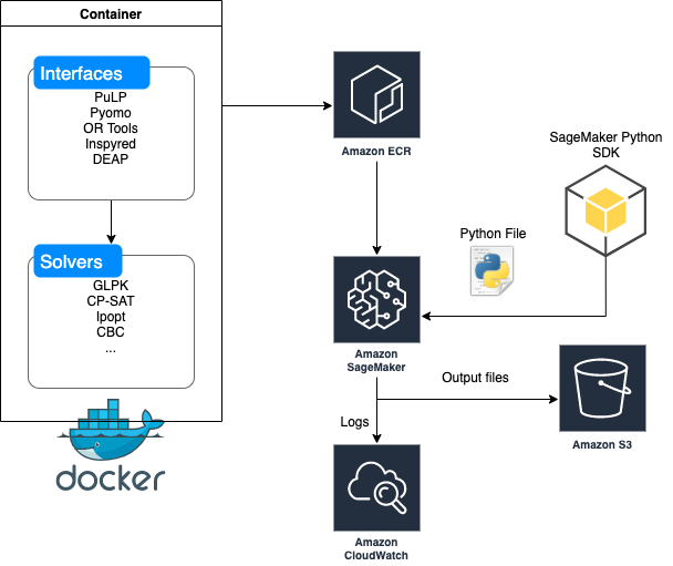
1. Build a Docker container that contains useful Python interfaces (such as Pyomo and PuLP) to optimization solvers (such as GLPK and CBC)
2. Build and push the image to a repository in Amazon Elastic Container Registry (Amazon ECR).
3. Use the SageMaker Python SDK (from a notebook or elsewhere with the right permissions) to point to the Docker image in Amazon ECR and send in a Python file with the actual optimization problem.
4. Monitor the logs in a notebook or Amazon CloudWatch Logs and obtain and outputs you need in a dedicated output folder that you specify in Amazon Simple Storage Service (Amazon S3).

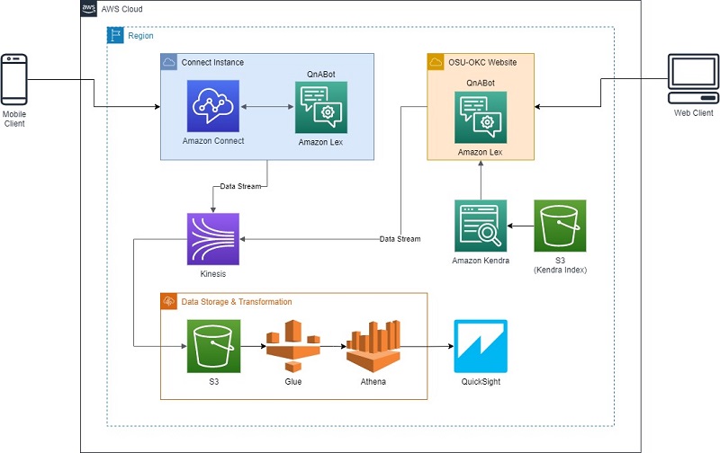
Schematically, this process looks like the following diagram.

Let’s get started!

Building and pushing a Docker container

Start with the following Dockerfile:

FROM continuumio/anaconda3

RUN pip install boto3 pandas scikit-learn pulp pyomo inspyred ortools scipy deap 

RUN conda install -c conda-forge ipopt coincbc glpk

ENV PYTHONUNBUFFERED=TRUE

ENTRYPOINT ["python"]

In this code, we install Python interfaces to solvers such as PuLP, Pyomo, Inspyred, OR-Tools, Scipy, and DEAP. For more information about these solvers, see the References section at the end of this post.

We then use the following commands from the notebook to build and push this container to Amazon ECR:

import boto3

account_id = boto3.client('sts').get_caller_identity().get('Account')
ecr_repository = 'sagemaker-opt-container'
tag = ':latest'
processing_repository_uri = '{}.dkr.ecr.{}.amazonaws.com/{}'.format(account_id, region, ecr_repository + tag)

# Create ECR repository and push docker image
!docker build -t $ecr_repository docker
!$(aws ecr get-login --region $region --registry-ids $account_id --no-include-email)
!aws ecr create-repository --repository-name $ecr_repository
!docker tag {ecr_repository + tag} $processing_repository_uri
!docker push $processing_repository_uri

Sample output for this command looks like the following code:

Sending build context to Docker daemon  2.048kB
Step 1/5 : FROM continuumio/anaconda3
 ---> 5fbf7bac70a0
Step 2/5 : RUN pip install boto3 pandas scikit-learn pulp pyomo inspyred ortools scipy deap
 ---> Using cache
 ---> 98864164a472
Step 3/5 : RUN conda install -c conda-forge ipopt coincbc glpk
 ---> Using cache
 ---> 1fde58988350
Step 4/5 : ENV PYTHONUNBUFFERED=TRUE
 ---> Using cache
 ---> 06cc27c84a9a
Step 5/5 : ENTRYPOINT ["python"]
 ---> Using cache
 ---> 0ae65a2ad5b9
Successfully built <code>
Successfully tagged sagemaker-opt-container:latest
WARNING! Using --password via the CLI is insecure. Use --password-stdin.
WARNING! Your password will be stored unencrypted in /home/ec2-user/.docker/config.json.
Configure a credential helper to remove this warning. See
https://docs.docker.com/engine/reference/commandline/login/#credentials-store

Login Succeeded

An error occurred (RepositoryAlreadyExistsException) when calling the CreateRepository operation: The repository with name 'sagemaker-opt-container' already exists in the registry with id '<account numnber>'
The push refers to repository [<account number>.dkr.ecr.<region>.amazonaws.com/sagemaker-opt-container]

8611989d: Preparing 
d960633d: Preparing 
db96c31c: Preparing 
ea6160d7: Preparing 
4bce66cd: Layer already exists latest: digest: sha256:<hash> size: 1379

Using the SageMaker Python SDK to start a job

Typically, we first initialize a SageMaker Processing ScriptProcessor as follows:

from sagemaker.processing import ScriptProcessor

script_processor = ScriptProcessor(command=['python'],
                image_uri=processing_repository_uri,
                role=role,
                instance_count=1,
                instance_type='ml.m5.xlarge')

Then we write a file (for this post, we always use a file called preprocessing.py) and run a processing job on SageMaker as follows:

from sagemaker.processing import ProcessingInput, ProcessingOutput

script_processor.run(code='preprocessing.py',
                      outputs=[ProcessingOutput(output_name='data',
                                                source='/opt/ml/processing/data')])

script_processor_job_description = script_processor.jobs[-1].describe()
print(script_processor_job_description)

Use case 1: Minimizing the cost of shipping goods through a distribution network

In this use case, American Steel, an Ohio-based steel manufacturing company, produces steel at its two steel mills located at Youngstown and Pittsburgh. The company distributes finished steel to its retail customers through the distribution network of regional and field warehouses.

The network represents shipment of finished steel from American Steel—two steel mills located at Youngstown (node 1) and Pittsburgh (node 2) to their field warehouses at Albany, Houston, Tempe, and Gary (nodes 6, 7, 8, and 9) through three regional warehouses located at Cincinnati, Kansas City, and Chicago (nodes 3, 4, and 5). Also, some field warehouses can be directly supplied from the steel mills.

The following table presents the minimum and maximum flow amounts of steel that may be shipped between different cities, along with the cost per 1,000 tons per month of shipping the steel. For example, the shipment from Youngstown to Kansas City is contracted out to a railroad company with a minimal shipping clause of 1,000 tons per month. However, the railroad can’t ship more than 5,000 tons per month due the shortage of rail cars.

The objective of transshipment problems in general and The American Steel Problem in particular is to minimize the cost of shipping goods through the network.

All the nodes have supply and demand, demand = 0 for supply nodes, supply = 0 for demand nodes, and supply = demand = 0 for transshipment nodes. The only constraints in the transshipment problem are flow conservation constraints. These constraints simply state that the flow of goods into a node must be greater than or equal to the flow of goods out of a node.

This problem can be formulated as follows:

%%writefile preprocessing.py

import argparse
import os
import warnings

"""
The American Steel Problem for the PuLP Modeller

Authors: Antony Phillips, Dr Stuart Mitchell  2007
"""

# Import PuLP modeller functions
from pulp import *

# List of all the nodes
Nodes = ["Youngstown",
         "Pittsburgh",
         "Cincinatti",
         "Kansas City",
         "Chicago",
         "Albany",
         "Houston",
         "Tempe",
         "Gary"]

nodeData = {# NODE        Supply Demand
         "Youngstown":    [10000,0],
         "Pittsburgh":    [15000,0],
         "Cincinatti":    [0,0],
         "Kansas City":   [0,0],
         "Chicago":       [0,0],
         "Albany":        [0,3000],
         "Houston":       [0,7000],
         "Tempe":         [0,4000],
         "Gary":          [0,6000]}

# List of all the arcs
Arcs = [("Youngstown","Albany"),
        ("Youngstown","Cincinatti"),
        ("Youngstown","Kansas City"),
        ("Youngstown","Chicago"),
        ("Pittsburgh","Cincinatti"),
        ("Pittsburgh","Kansas City"),
        ("Pittsburgh","Chicago"),
        ("Pittsburgh","Gary"),
        ("Cincinatti","Albany"),
        ("Cincinatti","Houston"),
        ("Kansas City","Houston"),
        ("Kansas City","Tempe"),
        ("Chicago","Tempe"),
        ("Chicago","Gary")]

arcData = { #      ARC                Cost Min Max
        ("Youngstown","Albany"):      [0.5,0,1000],
        ("Youngstown","Cincinatti"):  [0.35,0,3000],
        ("Youngstown","Kansas City"): [0.45,1000,5000],
        ("Youngstown","Chicago"):     [0.375,0,5000],
        ("Pittsburgh","Cincinatti"):  [0.35,0,2000],
        ("Pittsburgh","Kansas City"): [0.45,2000,3000],
        ("Pittsburgh","Chicago"):     [0.4,0,4000],
        ("Pittsburgh","Gary"):        [0.45,0,2000],
        ("Cincinatti","Albany"):      [0.35,1000,5000],
        ("Cincinatti","Houston"):     [0.55,0,6000],
        ("Kansas City","Houston"):    [0.375,0,4000],
        ("Kansas City","Tempe"):      [0.65,0,4000],
        ("Chicago","Tempe"):          [0.6,0,2000],
        ("Chicago","Gary"):           [0.12,0,4000]}

# Splits the dictionaries to be more understandable
(supply, demand) = splitDict(nodeData)
(costs, mins, maxs) = splitDict(arcData)

# Creates the boundless Variables as Integers
vars = LpVariable.dicts("Route",Arcs,None,None,LpInteger)

# Creates the upper and lower bounds on the variables
for a in Arcs:
    vars[a].bounds(mins[a], maxs[a])

# Creates the 'prob' variable to contain the problem data    
prob = LpProblem("American Steel Problem",LpMinimize)

# Creates the objective function
prob += lpSum([vars[a]* costs[a] for a in Arcs]), "Total Cost of Transport"

# Creates all problem constraints - this ensures the amount going into each node is at least equal to the amount leaving
for n in Nodes:
    prob += (supply[n]+ lpSum([vars[(i,j)] for (i,j) in Arcs if j == n]) >=
             demand[n]+ lpSum([vars[(i,j)] for (i,j) in Arcs if i == n])), "Steel Flow Conservation in Node %s"%n

# The problem data is written to an .lp file
prob.writeLP('/opt/ml/processing/data/' + 'AmericanSteelProblem.lp')

# The problem is solved using PuLP's choice of Solver
prob.solve()

# The status of the solution is printed to the screen
print("Status:", LpStatus[prob.status])

# Each of the variables is printed with it's resolved optimum value
for v in prob.variables():
    print(v.name, "=", v.varValue)

# The optimised objective function value is printed to the screen    
print("Total Cost of Transportation = ", value(prob.objective))

We solve this problem using the PuLP interface and its default solver GLPK using script_processor.run. Logs from this optimization job provide these solutions:

Status: Optimal
Route_('Chicago',_'Gary') = 4000.0
Route_('Chicago',_'Tempe') = 2000.0
Route_('Cincinatti',_'Albany') = 2000.0
Route_('Cincinatti',_'Houston') = 3000.0
Route_('Kansas_City',_'Houston') = 4000.0
Route_('Kansas_City',_'Tempe') = 2000.0
Route_('Pittsburgh',_'Chicago') = 3000.0
Route_('Pittsburgh',_'Cincinatti') = 2000.0
Route_('Pittsburgh',_'Gary') = 2000.0
Route_('Pittsburgh',_'Kansas_City') = 3000.0
Route_('Youngstown',_'Albany') = 1000.0
Route_('Youngstown',_'Chicago') = 3000.0
Route_('Youngstown',_'Cincinatti') = 3000.0
Route_('Youngstown',_'Kansas_City') = 3000.0
Total Cost of Transportation =  15005.0

Use case 2: Scheduling shifts of a set of nurses in a hospital

In the next example, a hospital supervisor must create a schedule for four nurses over a 3-day period, subject to the following conditions:

• Each day is divided into three 8-hour shifts
• Every day, each shift is assigned to a single nurse, and no nurse works more than one shift
• Each nurse is assigned to at least two shifts during the 3-day period

For more information about this scheduling use case, see Employee Scheduling.

This problem can be formulated as follows:

%%writefile preprocessing.py


from __future__ import print_function
from ortools.sat.python import cp_model



class NursesPartialSolutionPrinter(cp_model.CpSolverSolutionCallback):
    """Print intermediate solutions."""

    def __init__(self, shifts, num_nurses, num_days, num_shifts, sols):
        cp_model.CpSolverSolutionCallback.__init__(self)
        self._shifts = shifts
        self._num_nurses = num_nurses
        self._num_days = num_days
        self._num_shifts = num_shifts
        self._solutions = set(sols)
        self._solution_count = 0

    def on_solution_callback(self):
        if self._solution_count in self._solutions:
            print('Solution %i' % self._solution_count)
            for d in range(self._num_days):
                print('Day %i' % d)
                for n in range(self._num_nurses):
                    is_working = False
                    for s in range(self._num_shifts):
                        if self.Value(self._shifts[(n, d, s)]):
                            is_working = True
                            print('  Nurse %i works shift %i' % (n, s))
                    if not is_working:
                        print('  Nurse {} does not work'.format(n))
            print()
        self._solution_count += 1

    def solution_count(self):
        return self._solution_count




def main():
    # Data.
    num_nurses = 4
    num_shifts = 3
    num_days = 3
    all_nurses = range(num_nurses)
    all_shifts = range(num_shifts)
    all_days = range(num_days)
    # Creates the model.
    model = cp_model.CpModel()

    # Creates shift variables.
    # shifts[(n, d, s)]: nurse 'n' works shift 's' on day 'd'.
    shifts = {}
    for n in all_nurses:
        for d in all_days:
            for s in all_shifts:
                shifts[(n, d,
                        s)] = model.NewBoolVar('shift_n%id%is%i' % (n, d, s))

    # Each shift is assigned to exactly one nurse in the schedule period.
    for d in all_days:
        for s in all_shifts:
            model.Add(sum(shifts[(n, d, s)] for n in all_nurses) == 1)

    # Each nurse works at most one shift per day.
    for n in all_nurses:
        for d in all_days:
            model.Add(sum(shifts[(n, d, s)] for s in all_shifts) <= 1)

    # min_shifts_per_nurse is the largest integer such that every nurse
    # can be assigned at least that many shifts. If the number of nurses doesn't
    # divide the total number of shifts over the schedule period,
    # some nurses have to work one more shift, for a total of
    # min_shifts_per_nurse + 1.
    min_shifts_per_nurse = (num_shifts * num_days) // num_nurses
    max_shifts_per_nurse = min_shifts_per_nurse + 1
    for n in all_nurses:
        num_shifts_worked = sum(
            shifts[(n, d, s)] for d in all_days for s in all_shifts)
        model.Add(min_shifts_per_nurse <= num_shifts_worked)
        model.Add(num_shifts_worked <= max_shifts_per_nurse)

    # Creates the solver and solve.
    solver = cp_model.CpSolver()
    solver.parameters.linearization_level = 0
    # Display the first five solutions.
    a_few_solutions = range(5)
    solution_printer = NursesPartialSolutionPrinter(shifts, num_nurses,
                                                    num_days, num_shifts,
                                                    a_few_solutions)
    solver.SearchForAllSolutions(model, solution_printer)

    # Statistics.
    print()
    print('Statistics')
    print('  - conflicts       : %i' % solver.NumConflicts())
    print('  - branches        : %i' % solver.NumBranches())
    print('  - wall time       : %f s' % solver.WallTime())
    print('  - solutions found : %i' % solution_printer.solution_count())


if __name__ == '__main__':
    main()

We solve this problem using the OR-Tools interface and its CP-SAT solver with script_processor.run. Logs from this optimization job provide these solutions:

Solution 0
Day 0
  Nurse 0 does not work
  Nurse 1 works shift 0
  Nurse 2 works shift 1
  Nurse 3 works shift 2
Day 1
  Nurse 0 works shift 2
  Nurse 1 does not work
  Nurse 2 works shift 1
  Nurse 3 works shift 0
Day 2
  Nurse 0 works shift 2
  Nurse 1 works shift 1
  Nurse 2 works shift 0
  Nurse 3 does not work

Solution 1
Day 0
  Nurse 0 works shift 0
  Nurse 1 does not work
  Nurse 2 works shift 1
  Nurse 3 works shift 2
Day 1
  Nurse 0 does not work
  Nurse 1 works shift 2
  Nurse 2 works shift 1
  Nurse 3 works shift 0
Day 2
  Nurse 0 works shift 2
  Nurse 1 works shift 1
  Nurse 2 works shift 0
  Nurse 3 does not work

Solution 2
Day 0
  Nurse 0 works shift 0
  Nurse 1 does not work
  Nurse 2 works shift 1
  Nurse 3 works shift 2
Day 1
  Nurse 0 works shift 1
  Nurse 1 works shift 2
  Nurse 2 does not work
  Nurse 3 works shift 0
Day 2
  Nurse 0 works shift 2
  Nurse 1 works shift 1
  Nurse 2 works shift 0
  Nurse 3 does not work

Solution 3
Day 0
  Nurse 0 works shift 0
  Nurse 1 does not work
  Nurse 2 works shift 1
  Nurse 3 works shift 2
Day 1
  Nurse 0 works shift 2
  Nurse 1 works shift 1
  Nurse 2 does not work
  Nurse 3 works shift 0
Day 2
  Nurse 0 works shift 2
  Nurse 1 works shift 1
  Nurse 2 works shift 0
  Nurse 3 does not work

Solution 4
Day 0
  Nurse 0 does not work
  Nurse 1 works shift 0
  Nurse 2 works shift 1
  Nurse 3 works shift 2
Day 1
  Nurse 0 works shift 2
  Nurse 1 works shift 1
  Nurse 2 does not work
  Nurse 3 works shift 0
Day 2
  Nurse 0 works shift 2
  Nurse 1 works shift 1
  Nurse 2 works shift 0
  Nurse 3 does not work


Statistics
  - conflicts       : 37
  - branches        : 41231
  - wall time       : 0.367511 s
  - solutions found : 5184

Use case 3: Finding a trajectory for landing the Apollo 11 Lunar Module with the least amount of fuel

This example uses Pyomo and a simple model of a rocket to compute a control policy for a soft landing. The parameters used correspond to the descent of the Apollo 11 Lunar Module to the moon on July 20, 1969. For a rocket with a mass 𝑚 in vertical flight at altitude ℎ, a momentum balance yields the following model:

In this model, 𝑢 is the mass flow of propellant and 𝑣𝑒 is the velocity of the exhaust relative to the rocket. In this first attempt at modeling and control, we neglect the change in rocket mass due to fuel burn.

Fuel consumption can be calculated as the following:

We want to find a trajectory that minimizes fuel consumption:

This problem can be formulated as follows:

%%writefile preprocessing.py

import numpy as np

from pyomo.environ import *
from pyomo.dae import *

#Define constants ...
# lunar module
m_ascent_dry = 2445.0          # kg mass of ascent stage without fuel
m_ascent_fuel = 2376.0         # kg mass of ascent stage fuel
m_descent_dry = 2034.0         # kg mass of descent stage without fuel
m_descent_fuel = 8248.0        # kg mass of descent stage fuel

m_fuel = m_descent_fuel
m_dry = m_ascent_dry + m_ascent_fuel + m_descent_dry
m_total = m_dry + m_fuel

# descent engine characteristics
v_exhaust = 3050.0             # m/s
u_max = 45050.0/v_exhaust      # 45050 newtons / exhaust velocity

# landing mission specifications
h_initial = 100000.0           # meters
v_initial = 1520               # orbital velocity m/s
g = 1.62                       # m/s**2

m = ConcreteModel()
m.t = ContinuousSet(bounds=(0, 1))
m.h = Var(m.t)
m.u = Var(m.t, bounds=(0, u_max))
m.T = Var(domain=NonNegativeReals)

m.v = DerivativeVar(m.h, wrt=m.t)
m.a = DerivativeVar(m.v, wrt=m.t)

m.fuel = Integral(m.t, wrt=m.t, rule = lambda m, t: m.u[t]*m.T)
m.obj = Objective(expr=m.fuel, sense=minimize)

m.ode1 = Constraint(m.t, rule = lambda m, t: m_total*m.a[t]/m.T**2 == -m_total*g + v_exhaust*m.u[t])

m.h[0].fix(h_initial)
m.v[0].fix(-v_initial)

m.h[1].fix(0)    # land on surface
m.v[1].fix(0)    # soft landing

def solve(m):
    TransformationFactory('dae.finite_difference').apply_to(m, nfe=50, scheme='FORWARD')
    SolverFactory('ipopt').solve(m, tee=True)
    
solve(m)

We use the Pyomo interface and the nonlinear optimization solver Ipopt to solve this continuous-time, trajectory optimization problem. Logs from ScriptProcessor.run provide the following solution:

Ipopt 3.12.13: 

******************************************************************************
This program contains Ipopt, a library for large-scale nonlinear optimization.
 Ipopt is released as open source code under the Eclipse Public License (EPL).
         For more information visit http://projects.coin-or.org/Ipopt
******************************************************************************

This is Ipopt version 3.12.13, running with linear solver mumps.
NOTE: Other linear solvers might be more efficient (see Ipopt documentation).

Number of nonzeros in equality constraint Jacobian...:      448
Number of nonzeros in inequality constraint Jacobian.:        0
Number of nonzeros in Lagrangian Hessian.............:      154

Error in an AMPL evaluation. Run with "halt_on_ampl_error yes" to see details.
Error evaluating Jacobian of equality constraints at user provided starting point.
  No scaling factors for equality constraints computed!
Total number of variables............................:      201
                     variables with only lower bounds:        1
                variables with lower and upper bounds:       51
                     variables with only upper bounds:        0
Total number of equality constraints.................:      151
Total number of inequality constraints...............:        0
        inequality constraints with only lower bounds:        0
   inequality constraints with lower and upper bounds:        0
        inequality constraints with only upper bounds:        0

iter    objective    inf_pr   inf_du lg(mu)  ||d||  lg(rg) alpha_du alpha_pr  ls
   0  9.9999800e-05 5.00e+06 9.90e-01  -1.0 0.00e+00    -  0.00e+00 0.00e+00   0
   1r 9.9999800e-05 5.00e+06 9.99e+02   6.7 0.00e+00    -  0.00e+00 4.29e-14R  4
   2r 2.1397987e+02 5.00e+06 4.78e+08   6.7 2.14e+05    -  1.00e+00 6.83e-05f  1
   3r 2.1342176e+02 5.00e+06 1.36e+08   3.2 4.37e+04    -  7.16e-01 6.16e-01f  1
   4r 1.7048263e+02 4.99e+06 4.67e+07   3.2 1.60e+04    -  9.85e-01 4.16e-01f  1
   5r 1.5143799e+02 4.99e+06 2.50e+07   3.2 3.57e+03    -  5.88e-01 7.62e-01f  1
   6r 1.3041897e+02 4.99e+06 2.08e+07   3.2 1.89e+03    -  2.75e-01 8.14e-01f  1
   7r 1.1452223e+02 4.99e+06 3.17e+04   3.2 1.97e+03    -  9.78e-01 8.18e-01f  1
   8r 1.1168709e+02 4.99e+06 2.72e+05   3.2 3.36e-01   4.0 9.78e-01 1.00e+00f  1
   9r 1.0774716e+02 4.99e+06 1.66e+05   3.2 4.28e+03    -  9.36e-01 9.70e-02f  1
iter    objective    inf_pr   inf_du lg(mu)  ||d||  lg(rg) alpha_du alpha_pr  ls
  10r 8.7784873e+01 5.00e+06 5.08e+04   3.2 3.69e+03    -  8.74e-01 7.24e-01f  1
  11r 7.9008215e+01 5.00e+06 1.88e+04   2.5 1.09e+03    -  1.22e-01 8.35e-01h  1
  12r 1.1960245e+02 5.00e+06 4.34e+03   2.5 1.81e+03    -  6.76e-01 1.00e+00f  1
  13r 1.2344166e+02 5.00e+06 1.35e+03   1.8 1.66e+02    -  8.23e-01 1.00e+00f  1
  14r 2.0065756e+02 4.99e+06 6.85e+02   1.1 4.28e+03    -  4.26e-01 1.00e+00f  1
  15r 3.0115879e+02 4.99e+06 4.78e+01   1.1 9.69e+03    -  7.64e-01 1.00e+00f  1
  16r 3.0355974e+02 4.99e+06 5.30e+00   1.1 4.92e+00    -  1.00e+00 1.00e+00f  1
  17r 3.0555655e+02 4.99e+06 6.83e+02   0.4 7.49e+00    -  1.00e+00 1.00e+00f  1
  18r 4.4494526e+02 4.97e+06 2.28e+01   0.4 2.17e+04    -  8.05e-01 1.00e+00f  1
  19r 3.9588385e+02 4.97e+06 3.77e+00   0.4 4.73e+00    -  1.00e+00 1.00e+00f  1
iter    objective    inf_pr   inf_du lg(mu)  ||d||  lg(rg) alpha_du alpha_pr  ls
  20r 4.0158949e+02 4.97e+06 7.79e-02   0.4 5.70e-01    -  1.00e+00 1.00e+00h  1
  21r 4.0076180e+02 4.97e+06 9.88e+02  -1.0 1.80e+00    -  1.00e+00 1.00e+00f  1
  22r 5.4964501e+02 4.95e+06 7.59e+02  -1.0 1.57e+05    -  2.48e-01 2.32e-01f  1
  23r 5.5056601e+02 4.95e+06 7.57e+02  -1.0 1.21e+05    -  1.00e+00 3.02e-03f  1
  24r 5.5057553e+02 4.95e+06 7.57e+02  -1.0 1.09e+05    -  8.13e-01 3.34e-05f  1
  25r 5.5898777e+02 4.95e+06 7.00e+02  -1.0 3.82e+04    -  1.00e+00 7.48e-02f  1
  26r 6.0274077e+02 4.96e+06 3.93e+02  -1.0 3.53e+04    -  1.00e+00 4.39e-01f  1
  27r 6.0301192e+02 4.96e+06 3.90e+02  -1.0 1.98e+04    -  1.00e+00 7.83e-03f  1
  28r 6.0301418e+02 4.96e+06 3.89e+02  -1.0 1.61e+04    -  1.00e+00 9.62e-05f  1
  29r 5.9834909e+02 4.96e+06 3.71e+02  -1.0 3.63e+03    -  1.00e+00 1.85e-01f  1
iter    objective    inf_pr   inf_du lg(mu)  ||d||  lg(rg) alpha_du alpha_pr  ls
  30r 5.7601446e+02 4.95e+06 1.67e+00  -1.0 2.96e+03    -  1.00e+00 1.00e+00f  1
  31r 5.6977301e+02 4.95e+06 6.41e-02  -1.0 1.22e+00    -  1.00e+00 1.00e+00h  1
  32r 5.7024128e+02 4.95e+06 9.05e-05  -1.0 4.89e-02    -  1.00e+00 1.00e+00h  1
  33r 5.6989454e+02 4.95e+06 6.84e+02  -2.5 9.30e-02    -  1.00e+00 1.00e+00f  1
  34r 5.7613459e+02 4.94e+06 5.38e+02  -2.5 5.65e+04    -  4.67e-01 2.13e-01f  1
  35r 5.7617358e+02 4.94e+06 5.37e+02  -2.5 4.45e+04    -  1.00e+00 9.52e-04f  1
  36r 6.6264177e+02 4.90e+06 3.78e+01  -2.5 4.45e+04    -  6.62e-01 9.30e-01f  1
  37r 7.5101828e+02 4.90e+06 7.59e+01  -2.5 3.12e+03    -  1.25e-02 1.00e+00f  1
  38r 7.5705424e+02 4.90e+06 8.60e-02  -2.5 7.04e-01    -  1.00e+00 1.00e+00h  1
  39r 7.5713736e+02 4.90e+06 2.85e-05  -2.5 9.02e-03    -  1.00e+00 1.00e+00h  1
iter    objective    inf_pr   inf_du lg(mu)  ||d||  lg(rg) alpha_du alpha_pr  ls
  40r 7.5713093e+02 4.90e+06 4.90e+02  -5.7 6.76e-03    -  1.00e+00 9.99e-01f  1
  41r 1.0909809e+03 4.78e+06 4.67e+02  -5.7 2.54e+06    -  6.15e-02 4.62e-02f  1
  42r 1.0909867e+03 4.78e+06 4.67e+02  -5.7 2.42e+06    -  1.00e+00 9.55e-07f  1
  43r 1.5672936e+03 4.59e+06 8.15e+03  -5.7 2.42e+06    -  3.36e-03 7.69e-02f  1
  44r 1.7598365e+03 4.50e+06 8.17e+03  -5.7 2.24e+06    -  4.43e-08 4.23e-02f  1
  45r 5.7264420e+03 2.36e+06 4.60e+03  -5.7 2.14e+06    -  7.07e-02 1.00e+00f  1
  46  4.3546591e+03 2.35e+06 1.50e+01  -1.0 2.51e+08    -  3.52e-03 2.97e-03f  1
  47  3.7700543e+03 2.16e+06 1.94e+01  -1.0 2.87e+06    -  3.27e-01 8.10e-02f  1
  48  3.9963720e+03 1.02e+06 7.97e+00  -1.0 3.70e+05    -  3.47e-01 5.26e-01h  1
  49  4.0601733e+03 5.28e+05 5.09e+00  -1.0 1.57e+06    -  5.24e-03 4.85e-01h  1
iter    objective    inf_pr   inf_du lg(mu)  ||d||  lg(rg) alpha_du alpha_pr  ls
  50  4.0596593e+03 5.27e+05 3.53e+00  -1.0 4.32e+06    -  7.60e-01 1.81e-03h  1
  51  4.1577305e+03 9.40e+04 7.32e-01  -1.0 4.01e+05    -  9.09e-01 8.22e-01h  1
  52  4.1754490e+03 1.27e+01 4.74e-02  -1.0 5.08e+04    -  8.32e-01 1.00e+00h  1
  53  4.1752565e+03 7.78e-02 8.68e-07  -1.0 1.49e+04    -  1.00e+00 1.00e+00h  1
  54  4.1704409e+03 1.60e+00 3.18e-05  -2.5 1.16e+04    -  1.00e+00 1.00e+00f  1
  55  4.1704236e+03 6.98e-04 2.83e-08  -2.5 1.41e+03    -  1.00e+00 1.00e+00h  1
  56  4.1702897e+03 1.15e-03 2.31e-08  -3.8 2.98e+02    -  1.00e+00 1.00e+00f  1
  57  4.1702823e+03 3.63e-06 5.75e-11  -5.7 1.67e+01    -  1.00e+00 1.00e+00h  1
  58  4.1702822e+03 1.28e-09 1.62e-14  -8.6 2.04e-01    -  1.00e+00 1.00e+00h  1

Number of Iterations....: 58

                                   (scaled)                 (unscaled)
Objective...............:   4.1702822027548118e+03    4.1702822027548118e+03
Dual infeasibility......:   1.6235231869939369e-14    1.6235231869939369e-14
Constraint violation....:   1.2805685400962830e-09    1.2805685400962830e-09
Complementarity.........:   2.5079038009909822e-09    2.5079038009909822e-09
Overall NLP error.......:   2.5079038009909822e-09    2.5079038009909822e-09


Number of objective function evaluations             = 63
Number of objective gradient evaluations             = 16
Number of equality constraint evaluations            = 63
Number of inequality constraint evaluations          = 0
Number of equality constraint Jacobian evaluations   = 60
Number of inequality constraint Jacobian evaluations = 0
Number of Lagrangian Hessian evaluations             = 58
Total CPU secs in IPOPT (w/o function evaluations)   =      0.682
Total CPU secs in NLP function evaluations           =      0.002

EXIT: Optimal Solution Found.

Summary

We used various examples, front ends, and solvers to solve numerical optimization problems using SageMaker Processing. Next, try using Scipy.optimize, DEAP, or Inspyred to explore other examples. See the references in the next section for documentation and other examples to help solve your own business problems using SageMaker Processing. If you currently use SageMaker APIs for your machine learning projects, using SageMaker Processing for running optimization is a simple, obvious extension. However, consider that other compute options on AWS such as Lambda or Fargate may be more relevant when running some of these open source libraries for serverless optimization, especially when your team has this expertise. Lastly, open source libraries are provided as is, with minimal support whereas commercial libraries such as CPLEX and Gurobi are constantly being tuned for higher performance, and usually provide premium support.

References

• Training APIs: Processing
• https://pypi.org/project/PuLP/
• OR-Tools: Get Started Guides
• Pyomo Documentation 5.7.2
• inspyred: Recipes
• Optimization and root finding (scipy.optimize)
• DEAP documentation
• https://www.gurobi.com/
• CPLEX optimzer
• OR Tools code license
• PuLP code license
• Pyomo code license

About the Author

Shreyas Subramanian is a AI/ML specialist Solutions Architect, and helps customers by using Machine Learning to solve their business challenges using the AWS platform.

Read More

For many students, embarking on a higher education journey is an exciting time filled with new experiences. However, like anything new, it also can also bring plenty of questions to answer and obstacles to overcome. Oklahoma State University, Oklahoma City (OSU-OKC) recognized this, and was intent on providing a better solution to address student questions using machine learning (ML) technology from AWS.

They knew that if they could develop a solution that accurately anticipated their students’ needs and delivered timely and relevant information, they could boost their chances of attracting future students. After all, universities need students the same way businesses need customers.

“The first thing we wanted to address was the lack of visibility we had into customer sentiment at any given time,” says Michael Widell, Interim President at OKC-OSU. “Building on that, we also had a real focus on consistency and accuracy of information—it mattered to us that current and future students could rely on the information they were getting across school and faculty communication channels.”

The team identified conversational chatbots as a way to address the information gap that students face. ML-powered chatbots are dynamic, and help connect with students through the communication channels they prefer, whether that’s a website, phone, chatbot, or by asking an Alexa-enabled device.

With this in mind, OSU-OKC began working with AWS Professional Services in January 2020, and became the first university to deploy a call center using Amazon Connect and the QnABot.

Amazon Connect is a cloud contact center that provides a seamless experience across voice and chat for customers and agents. The QnABot is an open-source project that uses Amazon Lex to provide a conversational interface for your questions and answers, and can be applied to a host of communication channels, including websites, contact centers, chatbots, collaboration tools like Slack, and Amazon Alexa-enabled devices.

Deploying QnABot in the call center

Although OSU-OKC’s use of the QnABot evolved throughout 2020, its initial area of focus centered on boosting call center efficiency. They achieved this by automating answers to student FAQs, thereby delivering accurate and up-to-date information, reducing call hold times, and enabling human call center agents to focus on handling higher-value interactions.

The following diagram illustrates the solution architecture.

For OSU-OKC, QnABot simplified bot deployment and administration, allowing even non-technical users to maximize the impact of the solution by allowing them to:

• Deploy into their AWS account using AWS CloudFormation at the push of a button
• Use the Content Designer UI to add and edit content to make their bot smarter
• Integrate the bot with Amazon Kendra to tap into ML-powered enterprise search (for more information, see Using Kendra FAQ for question matching)
• Optionally customize the answers by mode; for example, use buttons and markdown for a rich web experience, and SSML for a rich voice experience
• Extend the bot using AWS Lambda hooks to fetch dynamic answers from external sources (for more information, see Extending QnABot with Lambda hook functions)
• Capture user feedback with “Thumbs Up” and “Thumbs Down” responses
• Use the built-in dashboards to see what questions people are asking, making it easy to add new features and functionality as users demand them
• Direct users to their website or a human agent on their helpdesk when the bot doesn’t have the answer to a question

Extending the QnABot to the website

After implementing the QnABot to assist agents inside their call center, OSU-OKC decided to extend the bot’s reach to the university’s website. They used the AWS open-source Amazon Lex Web UI project, a sample Amazon Lex Web UI that helps provide a full-featured web client for Amazon Lex chatbots.

After content was gathered from the campus, creating question and answer responses for the bot was an easy process. The content designer provided customization options that allowed for organization and readability. The built-in test features aided the tuning and development process by attributing a matching score to a response.

Shortly after expanding the QnABot to their website, OSU-OKC realized that providing more channels for students to interact with didn’t dilute engagement levels. In fact, they increased overall engagement from their student body and doubled the average number of conversations with students.

Adding the QnABot to the university website wasn’t a replacement for human interaction; it was an aid to increase quality interactions by reducing repetitive phone traffic. Try asking OSU-OKC bot, OKC Pete, some questions of your own via the university website.

OKC Pete on the university website

Equipping the QnABot with more responses

While QnABot answered high volumes of questions for students and delivered consistent service at scale, the OSU-OKC team learned a great deal about student sentiment by observing which questions the QnABot couldn’t answer.

For example, some questions highlighted how much prospective students knew about the campus and its resources. Incoming students asked about dorms when in fact the campus doesn’t have any student housing.

The team could use the QnABot’s Content Designer UI to continuously enhance the bot, and equip it with appropriate responses about student housing or any other campus resources. This helped students avoid a phone call, which freed call center agents to focus on more critical or higher-quality interactions.

This flexibility proved particularly helpful during the onset of the COVID-19 pandemic in the spring of 2020. OSU-OKC was able to rapidly expand the newly deployed QnABot’s knowledge base to include answers to many pandemic-related questions. Students and parents could quickly get answers to the questions that mattered to them via the QnABot-assisted university call center or via the website chatbot.

Scaling QnABot’s knowledge with Amazon Kendra

QnABot’s Content Designer UI allowed OSU-OKC to add new questions and answers to the bot when they identified a gap. However, the team also wanted to ensure that customers could still get answers when a question had not yet been added.

To achieve this, they used Amazon Kendra, a highly accurate intelligent search service. In the summer of 2020, the team at OSU-OKC integrated the QnABot with Amazon Kendra to enhance the accuracy and relevance of responses in the following ways:

• Use the document index in Amazon Kendra as an additional source of answers when a question and answer isn’t found in QnABot’s knowledge base. This allows QnABot to find answers to questions that may not have been added to its knowledge base, including unstructured data contained in word documents or PDFs that have been indexed by Amazon Kendra.
• Without extensive QnABot tuning, the natural language processing and reading comprehension capabilities of Amazon Kendra more accurately understand user queries, and its ML models expertly handle variations in how users phrase their questions to increase search accuracy and return relevant responses to user queries.

By using ML to automate the handling of common customer questions via their call center and website, OSU-OKC ensured consistent service levels even during their busiest time of year. Widell says, “During peak we can receive over 2,000 calls, which is too many for one agent to handle—however, since launching the QnABot, it’s supported over 34,000 conversations and saved 833 hours in staff time, while ensuring every customer received the same level of service and accuracy.”

Creating your own QnABot and integrating with Amazon Kendra

To get started on your own QnABot journey, see Create a Question and Answer Bot with Amazon Lex and Amazon Alexa. The section Turbocharging QnABot with Amazon Kendra outlines how to integrate QnABot with Amazon Kendra. If you want to follow OSU-OKC’s lead and add the QnABot to your website, you can take advantage of our companion Chatbot UI project.

As you think about configuration and deployment, consider the following options:

• Deploy the QnABot and Chatbot UI yourself (self-serve), using the project as is
• Make your own customizations and enhancements to the open-source code
• Follow OSU-OKC’s example and contact AWS Professional Services for expert help to customize and enhance QnABot, and to integrate with your own communication channels

For more information, watch the team at OSU-OKC present their QnABot solution at Re:Invent 2020.

Conclusion

The team at OSU-OKC is excited to build on the early success they have seen from deploying the QnABot, Amazon Kendra, and Amazon Lex. “For customers and students, this has been the most impactful technology that we’ve implemented,” Widell says.

Our overarching vision for ML technology will evolve student interactions from being transactional exchanges to becoming more meaningful experiences, allowing us to easily connect to customers, understand their needs, and serve them better. Widell adds, “In the future, we hope to expand our use of QnABot to provide personalized information to students as it relates to their academic schedules, advisement, and other relevant information related to their course of study.”

About the Authors

Bob Strahan is a Principal Solutions Architect in the AWS Language AI Services team.

Michael Widell is the Interim President at OSU-OKC. As an innovative agent of change he has worked to strengthen organizations through redesign and resource optimization, allowing individuals to excel, and deliver transformative products and services. In his career, Widell has also held leadership positions in the private sector for AT&T and key roles within the General Office of Walmart Inc. where he began his post collegiate career.

Read More

Training an accurate machine learning (ML) model requires many different steps, but none are potentially more important than data processing. Examples of processing steps include converting data to the input format expected by the ML algorithm, rescaling and normalizing, cleaning and tokenizing text, and many more. However, data processing at scale involves considerable operational overhead: managing complex infrastructure like processing clusters, writing code to tie all the moving pieces together, and implementing security and governance. Fortunately, AWS provides a wide variety of data processing options to suit every ML workload and teams’ preferred workflows. This set of options expanded even more at AWS re:Invent 2020, so now is the perfect time to examine how to choose between them.

In this post, we review the primary options and provide guidance on how to select one to match your use case and how your team prefers to work with Python, Spark, SQL, and other tools. Although the discussion centers around Amazon SageMaker for ML model building, training, and hosting, it’s equally applicable to workflows where other AWS services are used for these tasks, such as Amazon Personalize or Amazon Comprehend. The main assumption we make is that the decision is being made by those in data science, ML engineering, or MLOps roles. Other factors that are important in making the decision are team experience level, and inclination for writing code and managing infrastructure. Lower experience and inclination typically map to choosing a more fully managed option instead of a less managed or “roll your own” approach.

Prerequisite: Data Lake or Lake House

Before we dive deep into the options, there is a question we must answer: how do we reconcile our chosen option with the preferred technology choices of data engineering teams? Different tools may be suited to different roles; the tools a data scientist may prefer for an ML workflow may have little overlap with the tools used by a data engineer to support analytics workloads such as reporting. The good news is that AWS makes it very easy for these roles to pick their own tools and apply them to their organization’s data without conflict. The key is to create a data lake in Amazon Simple Storage Service (Amazon S3) at the center of the organization’s architecture for all data. This separates data and compute and avoids the problem of each team having individual data silos.

With a data lake in the center of the architecture, data engineering teams can apply their own tools for analytics workloads. At the same time, data science teams can also use their own separate tools to access the same data for ML workloads. Multiple separate processing clusters run by various teams can access the same data, always keeping in mind the need to retain the raw data in Amazon S3 for all teams as a source of truth. Additionally, use of a feature store for transformed data, such as Amazon SageMaker Feature Store, by data science teams helps delineate the boundary with data engineering, as well as provide benefits such as feature discovery, sharing, updating, and reuse.

As an alternative to a “classic” data lake, the teams might build on top of a Lake House Architecture, an evolution of the concept of a data lake. Featuring support for ACID transactions, this architecture enables multiple users to concurrently insert, delete, and modify rows across tables, while still allowing other users to simultaneously run analytical queries and ML models on the same datasets. AWS Lake Formation recently added new features to support the Lake House Architecture (currently in preview).

Now that we’ve solved the conundrum of enabling data engineering and data science teams to use their separate, preferred tools without conflict, let’s examine the data processing options for ML workloads on AWS.

Options overview

In this post, we review the following processing options. They’re in categories ranked by the following formula: (user friendliness for data scientists and ML engineers) x (usefulness for ML-specific tasks).

1. SageMaker managed features only
2. Low (or no) code solutions with other AWS services
3. Spark in Amazon EMR
4. Self-managed stack with Python or R

Keep in mind that these are not mutually exclusive; you can use them in various combinations to suit your team’s preferred workflow. For example, some teams may prefer to use SQL as much as possible, while others may use Spark for some tasks in addition to Python frameworks like Pandas. Another point to consider is that some services have built-in data visualization capabilities, while others do not and require use of other services for visualization. Let’s discuss the specifics of each option.

SageMaker managed features

SageMaker is a fully managed service that helps data scientists and developers prepare, build, train, and deploy high-quality ML models quickly by bringing together a broad set of capabilities purpose-built for ML. These capabilities include robust data processing features. For data processing and data preparation, you can use either Amazon SageMaker Data Wrangler or Amazon SageMaker Processing for the processing itself, and either Amazon SageMaker Studio or SageMaker notebook instances for data visualization. You can process datasets with sizes ranging from small to very large (petabytes) with SageMaker.

SageMaker Data Wrangler is a feature of SageMaker, enabled through SageMaker Studio, that makes it easy for data scientists and ML engineers to aggregate and prepare data for ML applications using a visual interface to accelerate data cleansing, exploration, and visualization. It allows you to easily connect to various data sources such as Amazon S3 and apply built-in transformations or custom transformations written in PySpark, Pandas, or SQL.

SageMaker Processing comes built in with SageMaker, and provides you with full control of your cluster resources such as instance count, type, and storage. It includes prebuilt containers for Spark and Scikit-learn, and offers an easy path for integrating your custom containers. For a “lift and shift” of an existing workload to SageMaker, SageMaker Processing may be a good fit. The following table compares SageMaker Processing and SageMaker Data Wrangler across some key dimensions.

The SageMaker option is ranked first due to its ease of use for data scientists and ML engineers, and its usefulness for ML-specific tasks; it was built from the ground up specifically to support ML workloads. However, several other options may be useful even though they weren’t developed solely for, or dedicated specifically to, ML workloads. Let’s review those options next.

Low (or no) code

This option involves several services that are serverless: infrastructure details and management are hidden under the hood. Additionally, there might be no need to write custom code, or in some cases, any code at all. This may lead to a relatively fast path to results, while potentially causing greater workflow friction by requiring you to switch between multiple services, UIs, and tools, and sacrificing some flexibility and ability to customize. For our purposes, we consider a solution that requires SQL queries to be a low code solution, and one that doesn’t require any code, even SQL, to be a no code solution.

For example, one low code possibility involves Amazon Athena, a serverless interactive query service, for transforming data using standard SQL queries, in combination with Amazon QuickSight, a serverless BI tool that offers no code, built-in visualizations. When evaluating this powerful combination, consider whether your data transformations can be accomplished with SQL. On the visualization side, an alternative to QuickSight is to use a library such as PyAthena to run the queries in SageMaker notebooks with Python code and visualize the results there.

Another low code possibility involves AWS Glue, a serverless ETL service that catalogs your data and offers built-in transforms, along with the ability to write custom PySpark code. For visualizations, besides QuickSight, you can attach either SageMaker or Zeppelin notebooks to an AWS Glue development endpoint. Choosing between AWS Glue and Athena comes down to a team’s preference for using SQL versus PySpark code (in the case when AWS Glue built-in transforms don’t fully cover the desired set of data transforms).

A no code possibility is AWS Glue DataBrew, a serverless visual data preparation tool, to transform data, combined with either the SageMaker console to start model training jobs using built-in algorithms such as XGBoost, or the SageMaker Studio UI to start AutoML model training jobs with SageMaker Autopilot. With many built-in transformations and built-in visualizations, DataBrew covers both data processing and data visualization. However, if your dataset requires custom transformations other than the built-in ones, you need to pair DataBrew with another solution that allows you to write custom code. Autopilot automatically performs typical featurization of data (such as one-hot encoding of categorical values) as part of its AutoML pipeline, so you might find the set of transformations in DataBrew sufficient if paired with Autopilot. The following table provides a more detailed comparison.

Spark in Amazon EMR

Many organizations use Spark for data processing and other purposes, such as the basis for a data warehouse. In these situations, Spark clusters are typically run in Amazon EMR, a managed service for Hadoop-ecosystem clusters, which eliminates the need to do your own setup, tuning, and maintenance. From the perspective of a data scientist or ML engineer, Spark in Amazon EMR may be considered in the following circumstances:

• Spark is already used for a data warehouse or other application with a persistent cluster. Unlike the other options we described, which only provision transient resources, Amazon EMR also enables creation of persistent clusters to support analytics applications.
• The team already has a complete end-to-end pipeline in Spark and also the skillset and inclination to run a persistent Spark cluster for the long term. Otherwise, the SageMaker and AWS Glue options for Spark generally are preferable.

Another consideration is the wider range of instance types offered by Amazon EMR, including AWS Graviton2 processors and Amazon EC2 Spot Instances for cost optimization.

For visualization with Amazon EMR, there are several choices. To keep your primary ML workflow within SageMaker, use SageMaker Studio and its built-in SparkMagic kernel to connect to Amazon EMR. You can start to query, analyze, and process data with Spark in a few steps. For added security, you can connect to EMR clusters using Kerberos authentication. Amazon EMR also features other integrations with SageMaker, for example you can start a SageMaker model training job from a Spark pipeline in Amazon EMR. Another visualization possibility is to use Amazon EMR Studio (preview), which provides access to fully managed Jupyter notebooks, and includes the ability to log in via AWS Single Sign-On (AWS SSO). However, EMR Studio lacks the many SageMaker-specific UI integrations of SageMaker Studio.

There are other factors to consider when evaluating this option. Spark is based on the Scala/Java stack, with all the problems that entails in regard to dependency management and JVM issues that may be unfamiliar to data scientists. Also keep in mind that Spark’s PySpark API has often lagged behind its primary API in Scala, which is a language less familiar to data scientists. In this regard, if you prefer the alternative Dask framework for your workloads, you can install Dask on your EMR clusters.

Self-managed stack using Python or R

For this option, teams roll their own solutions using Amazon Elastic Compute Cloud (Amazon EC2) compute resources, or the container services Amazon Elastic Container Service (Amazon ECS) or Amazon Elastic Kubernetes Service (Amazon EKS).  Integration with SageMaker is most conveniently achieved using the Amazon SageMaker Python SDK. Any machine with AWS Identity and Access Management (IAM) permissions to SageMaker can use the SageMaker Python SDK to invoke SageMaker functionality for model building, training, tuning, deployment, and more.

This option provides the most flexibility to mix and match any data processing tools and frameworks. It also offers access to the widest range of EC2 instance types and storage options. In addition to the possibility of using Spot Instances similarly to Amazon EMR, you can also use this option with the flexible pricing model of AWS Savings Plans. These plans can be applied not only to Amazon EC2 resources, but also to serverless compute AWS Lambda resources, and serverless compute engine AWS Fargate resources.

However, keep in mind in regard to user-friendliness for data scientists and ML engineers, this option requires them to manage low-level infrastructure, a task better suited to other roles. Also, with respect to usefulness for ML-specific tasks, although there are many frameworks and tools that can be layered on top of these services to make management easier and provide specific functionality for ML workloads, this option is still far less managed than the preceding options. It requires more personnel time to manage, tune, maintain infrastructure and dependencies, and write code to fill functionality gaps. As a result, this option also is likely to prove the most costly in the long run.

Review and conclusion

Your choice of a data processing option for ML workloads typically depends on your team’s preference for tools (Spark, SQL, or Python) and inclination for writing code and managing infrastructure. The following table summarizes the options across several relevant dimensions. The first column emphasizes that separate services or features may be used for processing and related visualization, and the third column refers to resources used to process data rather than for visualization, which tends to happen on lighter-weight resources.

Workloads evolve over time, and you don’t need to be locked in to one set of tools forever. You can mix and match according to your use case. When you use Amazon S3 at the center of your data lake and the fully managed SageMaker service for core ML workflow steps, it’s easy to switch tools as needed or desired to accommodate the latest technologies. Whichever option you choose now, AWS provides the flexibility to evolve your tool chain to best fit the then-current data processing needs of your ML workloads.

About the Author

Brent Rabowsky focuses on data science at AWS, and leverages his expertise to help AWS customers with their own data science projects.

Read More

JavaScript Object Notation (JSON) is a schema-less, lightweight format for storing and transporting data. It’s a text-based, self-describing representation of structured data that is based on key-value pairs. JSON is supported either natively or through libraries in most major programming languages, and is commonly used to exchange information between web clients and web servers. Over the last 15 years, JSON has become ubiquitous on the web and is the format of choice for almost all web services.

To reach more users, you often want to localize your content and applications that may be in JSON format. This post shows you a serverless approach for easily translating JSON documents using Amazon Translate. Serverless architecture is ideal because it is event-driven and can automatically scale, making it a cost effective solution. In this approach, JSON tags are left as they are, and the content within those tags is translated. This allows you to preserve the context of the text, so that translations can be handled with greater precision. The approach presented here was recently used by a large higher education customer of AWS for translating media documents that are in JSON format.

Amazon Translate is a neural machine translation service that delivers fast, high-quality, affordable, and customizable language translation. Neural machine translation uses deep learning models to deliver more accurate and natural-sounding translation than traditional statistical and rule-based translation algorithms. The translation service is trained on a wide variety of content across different use cases and domains to perform well on many kinds of content. Its asynchronous batch processing capability enables you to translate a large collection of text, HTML, and OOXML documents with a single API call.

In this post, we walk you through creating an automated and serverless pipeline for translating JSON documents using Amazon Translate.

Solution overview

Amazon Translate currently supports the ability to ignore tags and only translate text content in XML documents. In this solution, we therefore first convert JSON documents to XML documents, use Amazon Translate to convert text content in the XML document, and then covert the XML document back to JSON.

The solution uses serverless technologies and managed services to provide maximum scalability and cost-effectiveness. In addition to Amazon Translate, the solution uses the following services:

• AWS Lambda – Runs code in response to triggers such as changes in data, changes in application state, or user actions. Because services like Amazon S3 and Amazon SNS can directly trigger a Lambda function, you can build a variety of real-time serverless data-processing systems.
• Amazon Simple Notification Service (Amazon SNS) – Enables you to decouple microservices, distributed systems, and serverless applications with a highly available, durable, secure, fully managed publish/subscribe messaging service.
• Amazon Simple Storage Service (Amazon S3) – Stores your documents and allows for central management with fine-tuned access controls.
• AWS Step Functions – Coordinates multiple AWS services into serverless workflows.

Solution architecture

The architecture workflow contains the following steps:

1. Users upload one or more JSON documents to Amazon S3.
2. The Amazon S3 upload triggers a Lambda function.
3. The function converts the JSON documents into XML, stores them in Amazon S3, and invokes Amazon Translate in batch mode to translate the XML documents texts into the target language.
4. The Step Functions-based job poller polls for the translation job to complete.
5. Step Functions sends an SNS notification when the translation is complete.
6. A Lambda function reads the translated XML documents in Amazon S3, converts them to JSON documents, and stores them back in Amazon S3.

The following diagram illustrates this architecture.

Deploying the solution with AWS CloudFormation

The first step is to use an AWS CloudFormation template to provision the necessary resources needed for the solution, including the AWS Identity and Access Management (IAM) roles, IAM policies, and SNS topics.

1. Launch the AWS CloudFormation template by choosing Launch Stack (this creates the stack the us-east-1 Region):
   

2. For Stack name, enter a unique stack name for this account; for example, translate-json-document.
3. For SourceLanguageCode, enter the language code for the current language of the JSON documents; for example, en for English.
4. For TargetLanguageCode, enter the language code that you want your translated documents in; for example, es for Spanish.

For more information about supported languages, see Supported Languages and Language Codes.

5. For TriggerFileName, enter the name of the file that triggers the translation serverless pipeline; the default is triggerfile.
6. In the Capabilities and transforms section, select the check boxes to acknowledge that AWS CloudFormation will create IAM resources and transform the AWS Serverless Application Model (AWS SAM) template.

AWS SAM templates simplify the definition of resources needed for serverless applications. When deploying AWS SAM templates in AWS CloudFormation, AWS CloudFormation performs a transform to convert the AWS SAM template into a CloudFormation template. For more information, see Transform.

7. Choose Create stack.

The stack creation may take up to 20 minutes, after which the status changes to CREATE_COMPLETE. You can see the name of the newly created S3 bucket on the Outputs tab.

Translating JSON documents

To translate your documents, upload one or more JSON documents to the input folder of the S3 bucket you created in the previous step. For this post, we use the following JSON file:

{
    "firstName": "John",
    "lastName": "Doe",
    "isAlive": true,
    "age": 27,
    "address": {
      "streetAddress": "100 Main Street",
      "city": "Anytown",
      "postalCode": "99999-9999"
    },
    "phoneNumbers": [
      {
        "type": "home",
        "number": "222 555-1234"
      },
      {
        "type": "office",
        "number": "222 555-4567"
      }
    ],
    "children": ["Richard Roe", "Paulo Santos"],
    "spouse": "Jane Doe"
}

After you upload all the JSON documents, upload the file that triggers the translation workflow. This file can be a zero-byte file, but the filename should match the TriggerFileName parameter in the CloudFormation stack. The default name for the file is triggerfile.

This upload event triggers the Lambda function <Stack name>-S3FileEventProcessor-<Random string>, which converts the uploaded JSON documents into XML and places them in the xmlin folder of the S3 bucket. The function then invokes the Amazon Translate startTextTranslationJob, with the xmlin folder in the S3 bucket location as the input location and the xmlout folder as the output location for the translated XML files.

The following code is the processRequest method in the <Stack name>-S3FileEventProcessor-<Random string> Lambda function:

def processRequest(request):
    output = ""
    logger.info("request: {}".format(request))

    bucketName = request["bucketName"]
    sourceLanguageCode = request["sourceLanguage"]
    targetLanguageCode = request["targetLanguage"]
    access_role = request["access_role"]
    triggerFile = request["trigger_file"]
    try:
        # Filter only the JSON files for processing
        objs = S3Helper().getFilteredFileNames(bucketName,"input/","json")
        for obj in objs:
            try:
                content = S3Helper().readFromS3(bucketName,obj)
                logger.debug(content)
                jsonDocument = json.loads(content)
                print(jsonDocument)
                # Convert the JSON document into XML
                outputXML = json2xml.Json2xml(jsonDocument, attr_type=False).to_xml()
                logger.debug(outputXML)
                newObjectKey = "xmlin/{}.xml".format(FileHelper.getFileName(obj))
                # Store the XML in the S3 location for Translation
                S3Helper().writeToS3(str(outputXML),bucketName,newObjectKey)   
                output = "Output Object: {}/{}".format(bucketName, newObjectKey)
                logger.debug(output)
                # Rename the JSON files to prevent reprocessing
                S3Helper().renameObject(bucketName,obj,"{}.processed".format(obj))
            except ValueError:
                logger.error("Error occured loading the json file:{}".format(obj))
            except ClientError as e:
                logger.error("An error occured with S3 Bucket Operation: %s" % e)
        # Start the translation batch job using Amazon Translate
        startTranslationJob(bucketName,sourceLanguageCode,targetLanguageCode,access_role)
        S3Helper().deleteObject(bucketName,"input/{}".format(triggerFile))
    except ClientError as e:
        logger.error("An error occured with S3 Bucket Operation: %s" % e)

The Amazon Translate job completion SNS notification from the job poller triggers the Lambda function <Stack name>-TranslateJsonJobSNSEventProcessor-<Random string>. The function converts the XML document created by the Amazon Translate batch job to JSON documents in the output folder of the S3 bucket with the following naming convention: TargetLanguageCode-<inputJsonFileName>.json.

The following code shows the JSON document translated in Spanish.

{
    "firstName": "John",
    "lastName": "Cierva",
    "isAlive": "Es verdad",
    "age": "27",
    "address": {
        "streetAddress": "100 Calle Principal",
        "city": "En cualquier ciudad",
        "postalCode": "99999-9999"
    },
    "phoneNumbers": {
        "item": [
            {
                "type": "hogar",
                "number": "222 555-1234"
            },
            {
                "type": "oficina",
                "number": "222 555-4567"
            }
        ]
    },
    "children": {
        "item": [
            "Richard Roe",
            "Paulo Santos"
        ]
    },
    "spouse": "Jane Doe"
}

The following code is the processRequest method containing the logic in the <Stack name>-TranslateJsonJobSNSEventProcessor-<Random string> Lambda function:

def processRequest(request):
    output = ""
    logger.debug("request: {}".format(request))
    up = urlparse(request["s3uri"], allow_fragments=False)
    accountid = request["accountId"]
    jobid =  request["jobId"]
    bucketName = up.netloc
    objectkey = up.path.lstrip('/')
    # choose the base path for iterating within the translated files for the specific job
    basePrefixPath = objectkey  + accountid + "-TranslateText-" + jobid + "/"
    languageCode = request["langCode"]
    logger.debug("Base Prefix Path:{}".format(basePrefixPath))
    # Filter only the translated XML files for processing
    objs = S3Helper().getFilteredFileNames(bucketName,basePrefixPath,"xml")
    for obj in objs:
        try:
            content = S3Helper().readFromS3(bucketName,obj)
            logger.debug(content)
            #Convert the XML file to Dictionary object
            data_dict = xmltodict.parse(content)
            #Generate the Json content from the dictionary
            data_dict =  data_dict["all"]
            flatten_dict = {k: (data_dict[k]["item"] if (isinstance(v,dict) and len(v.keys()) ==1 and "item" in v.keys())  else v) for (k,v) in data_dict.items()}
            json_data = json.dumps(flatten_dict,ensure_ascii=False).encode('utf-8')
            logger.debug(json_data)
            newObjectKey = "output/{}.json".format(FileHelper.getFileName(obj))
            #Write the JSON object to the S3 output folder within the bucket
            S3Helper().writeToS3(json_data,bucketName,newObjectKey)   
            output = "Output Object: {}/{}".format(bucketName, newObjectKey)
            logger.debug(output)
        except ValueError:
            logger.error("Error occured loading the json file:{}".format(obj))
        except ClientError as e:
            logger.error("An error occured with S3 bucket operations: %s" % e)
        except :
            e = sys.exc_info()[0]
            logger.error("Error occured processing the xmlfile: %s" % e)
    objs = S3Helper().getFilteredFileNames(bucketName,"xmlin/","xml")
    if( request["delete_xmls"] and request["delete_xmls"] == "true") :
        for obj in objs:
            try:
                logger.debug("Deleting temp xml files {}".format(obj))
                S3Helper().deleteObject(bucketName,obj)
            except ClientError as e:
                logger.error("An error occured with S3 bucket operations: %s" % e)
            except :
                e = sys.exc_info()[0]
                logger.error("Error occured processing the xmlfile: %s" % e)

For any pipeline failures, check the Amazon CloudWatch Logs for the corresponding Lambda function and look for potential errors that caused the failure.

To do a translation for a different source-target language combination, you can update the SOURCE_LANG_CODE and TARGET_LANG_CODE environment variable for the <Stack name>-S3FileEventProcessor-<Random string> Lambda function and trigger the solution pipeline by uploading JSON documents and the TriggerFileName into the input folder of the S3 bucket.

All code used in this post is available in the GitHub repo. If you want to build your own pipeline and don’t need to use the CloudFormation template provided, you can use the file s3_event_handler.py under the directory translate_json in the GitHub repo. That file carries code to convert a JSON file into XML as well as to call the Amazon Translate API. The code for converting translated XML back to JSON format is available in the file sns_event_handler.py.

Conclusion

In this post, we demonstrated how to translate JSON documents using Amazon Translate asynchronous batch processing.

You can easily integrate the approach into your own pipelines as well as handle large volumes of JSON text given the scalable serverless architecture. This methodology works for translating JSON documents between over 70 languages that are supported by Amazon Translate (as of this writing). Because this solution uses asynchronous batch processing, you can customize your machine translation output using parallel data. For more information on using parallel data, see Customizing Your Translations with Parallel Data (Active Custom Translation). For a low-latency, low-throughput solution translating smaller JSON documents, you can perform the translation through the real-time Amazon Translate API.

For further reading, we recommend the following:

• Asynchronous Batch Processing with Amazon Translate
• Translating documents with Amazon Translate, AWS Lambda, and the new Batch Translate API
• Getting a batch job completion message from Amazon Translate
• Amazon Translate FAQs

About the Authors

Siva Rajamani is a Boston-based Enterprise Solutions Architect for AWS. He enjoys working closely with customers and supporting their digital transformation and AWS adoption journey. His core areas of focus are serverless, application integration, and security. Outside of work, he enjoys outdoors activities and watching documentaries.

Raju Penmatcha is a Senior AI/ML Specialist Solutions Architect at AWS. He works with education, government, and non-profit customers on machine learning and artificial intelligence related projects, helping them build solutions using AWS. When not helping customers, he likes traveling to new places with his family.

Read More