Monthly Archives: February 2021

The ability to rapidly iterate and train machine learning (ML) models is key to deriving business value from ML workloads. Because ML models often have many tunable parameters (known as hyperparameters) that can influence the model’s ability to effectively learn, data scientists often use a technique known as hyperparameter optimization (HPO) to achieve the best-performing model against a certain predefined metric. Depending on the number of hyperparameters and the size of the search space, finding the best model can require thousands or even tens of thousands of training runs. Real-world problems that often require extensive HPO include image segmentation for modeling vehicular traffic for autonomous driving, developing algorithmic trading strategies based on historical financial data, or building fraud detection models on transaction data. Amazon SageMaker provides a built-in HPO algorithm that removes the undifferentiated heavy lifting required to build your own HPO algorithm. This post shows how to batch your HPO jobs to maximize the number of jobs you can run in parallel, thereby reducing the total time it takes to effectively cover the desired parameter space and obtain the best-performing models.

Before diving into the batching approach on Amazon SageMaker, let’s briefly review the state-of-the-art [1]. There are a large number of HPO algorithms, ranging from random or grid search, Bayesian search, and hand tuning, where researchers use their domain knowledge to tune parameters to population-based training inspired from genetic algorithms. For deep learning models, however, even training a single training run can be time consuming. In that case, it becomes important to have an aggressive early stopping strategy, which ends trials in search spaces that are unlikely to produce good results. Several strategies like successive halving or asynchronous successive halving use multi-arm bandits to trade-off between exploration (trying out different parameter combinations) versus exploitation (allowing a training run to converge). Finally, to help developers quickly iterate with these approaches, there are a number of tools, such as SageMaker HPO, Ray, HyperOpt, and more. In this post, you also see how you can bring one of the most popular HPO tools, Ray Tune, to SageMaker.

Use case: Predicting credit card loan defaults

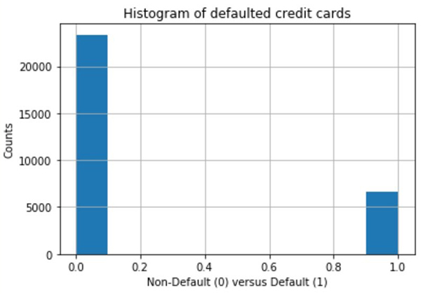
To demonstrate this on a concrete example, imagine that you’re an ML engineer working for a bank, and you want to predict the likelihood of a customer defaulting on their credit card payments. To train a model, you use historical data available from the UCI repository. All the code developed in this post is made available on GitHub. The notebook covers the data preprocessing required to prep the raw data for training. Because the number of defaults is quite small (as shown in the following graph), we split the dataset into train and test, and upsample the training data to 50/50 default versus non-defaulted loans.

Then we upload the datasets to Amazon Simple Storage Service (Amazon S3). See the following code:

#Upload Training and test data into S3
train_s3 = sagemaker_session.upload_data(path='./train_full_split/', key_prefix=prefix + '/train')
print(train_s3)
test_s3 = sagemaker_session.upload_data(path='./test_full_split/', key_prefix=prefix + '/test')
print(test_s3)

Although SageMaker provides many built-in algorithms, such as XGBoost, in this post we demonstrate how to apply HPO to a custom PyTorch model using the SageMaker PyTorch training container using script mode. You can then adapt this to your own custom deep learning code. Furthermore, we will demonstrate how you can bring custom metrics to SageMaker HPO.

When dealing with tabular data, it’s helpful to shard your dataset into smaller files to avoid long data loading times, which can starve your compute resources and lead to inefficient CPU/GPU usage. We create a custom Dataset class to fetch our data and wrap this in the DataLoader class to iterate over the dataset. We set the batch size to 1, because each batch consists of 10,000 rows, and load it using Pandas.

Our model is a simple feed-forward neural net, as shown in the following code snippet:

class Net(nn.Module):
    def __init__(self, inp_dimension):
        super().__init__()
        self.fc1 = nn.Linear(inp_dimension, 500)
        self.drop = nn.Dropout(0.3)
        self.bn1 = nn.BatchNorm1d(500)
        self.bn2=nn.BatchNorm1d(250)
        self.fc2 = nn.Linear(500, 250)
        self.fc3 = nn.Linear(250, 100)
        self.bn3=nn.BatchNorm1d(100)
        self.fc4 = nn.Linear(100,2)
        


    def forward(self, x):
        x = x.squeeze()
        x = F.relu(self.fc1(x.float()))
        x = self.drop(x)
        x = self.bn1(x)
        x = F.relu(self.fc2(x))
        x = self.drop(x)
        x = self.bn2(x)
        x = F.relu(self.fc3(x))
        x = self.drop(x)
        x = self.bn3(x)
        x = self.fc4(x)
        # last layer converts it to binary classification probability
        return F.log_softmax(x, dim=1)

As shown in the Figure above, the dataset is highly imbalanced and as such, model accuracy isn’t the most useful evaluation metric, because a baseline model that predicts all customers won’t default on their payments will have high accuracy. A more useful metric is the AUC, which is the area under the receiver operator characteristic (ROC) curve that aims to minimize the number of false positives while maximizing the number of true positives. A false positive (model incorrectly predicting a good customer will default on their payment) can cause the bank to lose revenue by denying credit cards to customers. To make sure that your HPO algorithm can optimize on a custom metric such as the AUC or F1-score, you need to log those metrics into STDOUT, as shown in the following code:

def test(model, test_loader, device, loss_optim):
    model.eval()
    test_loss = 0
    correct = 0
    fulloutputs = []
    fulltargets = []
    fullpreds = []
    with torch.no_grad():
        for i, (data, target) in enumerate(test_loader):
            data, target = data.to(device), target.to(device)
            output = model(data)
            target = target.squeeze()
            test_loss += loss_optim(output, target).item()  # sum up batch loss
            pred = output.max(1, keepdim=True)[1]  # get the index of the max log-probability
            correct += pred.eq(target.view_as(pred)).sum().item()
            fulloutputs.append(output.cpu().numpy()[:, 1])
            fulltargets.append(target.cpu().numpy())
            fullpreds.append(pred.squeeze().cpu())

    i+=1
    test_loss /= i
    logger.info("Test set Average loss: {:.4f}, Test Accuracy: {:.0f}%;n".format(
            test_loss, 100. * correct / (len(target)*i)
        ))
    fulloutputs = [item for sublist in fulloutputs for item in sublist]
    fulltargets = [item for sublist in fulltargets for item in sublist]
    fullpreds = [item for sublist in fullpreds for item in sublist]
    logger.info('Test set F1-score: {:.4f}, Test set AUC: {:.4f} n'.format(
        f1_score(fulltargets, fullpreds), roc_auc_score(fulltargets, fulloutputs)))

Now we’re ready to define our SageMaker estimator and define the parameters for the HPO job:

estimator = PyTorch(entry_point="train_cpu.py",
                    role=role,
                    framework_version='1.6.0',
                    py_version='py36',
                    source_dir='./code',
                    output_path = f's3://{bucket}/{prefix}/output',
                    instance_count=1, 
                    sagemaker_session=sagemaker_session,
                    instance_type='ml.m5.xlarge', 
                    hyperparameters={
                        'epochs': 10, # run more epochs for HPO.
                        'backend': 'gloo' #gloo for cpu, nccl for gpu
                    }
            )
            
#specify the hyper-parameter ranges           
hyperparameter_ranges = {'lr': ContinuousParameter(0.001, 0.1),
                         'momentum': CategoricalParameter(list(np.arange(0, 10)/10))}

inputs ={'training': train_s3,
         'testing':test_s3}

#specify the custom HPO metric
objective_metric_name = 'test AUC'
objective_type = 'Maximize'
metric_definitions = [{'Name': 'test AUC',
                       'Regex': 'Test set AUC: ([0-9\.]+)'}]   #note that the regex must match your test function above      
estimator.fit({'training': train_s3,
                'testing':test_s3},
             wait=False)

We pass in the paths to the training and test data in Amazon S3.

With the setup in place, let’s now turn to running multiple HPO jobs.

Parallelizing HPO jobs

To run multiple hyperparameter tuning jobs in parallel, we must first determine the tuning strategy. SageMaker currently provides a random and Bayesian optimization strategy. For random strategy, different HPO jobs are completely independent of one another, whereas Bayesian optimization treats the HPO problem as a regression problem and makes intelligent guesses about the next set of parameters to pick based on the prior set of trials.

First, let’s review some terminology:

• Trials – A trial corresponds to a single training job with a set of fixed values for the hyperparameters
• max_jobs – The total number of training trials to run for that given HPO job
• max_parallel_jobs – The maximum concurrent running trials per HPO job

Suppose you want to run 10,000 total trials. To minimize the total HPO time, you want to run as many trials as possible in parallel. This is limited by the availability of a particular Amazon Elastic Compute Cloud (Amazon EC2) instance type in your Region and account. If you want to modify or increase those limits, speak to your AWS account representatives.

For this example, let’s suppose that you have 20 ml.m5.xlarge instances available. This means that you can simultaneously run 20 trials of one instance each. Currently, without increasing any limits, SageMaker limits max_jobs to 500 and max_parallel_jobs to 10. This means that you need to run a total of 10,000/500 = 20 HPO jobs. Because you can run 20 trials and max_parallel_jobs is 10, you can maximize the number of simultaneous HPO jobs running by running 20/10 = 2 HPO jobs in parallel. So one approach to batch your code is to always have two jobs running, until you meet your total required jobs of 20.

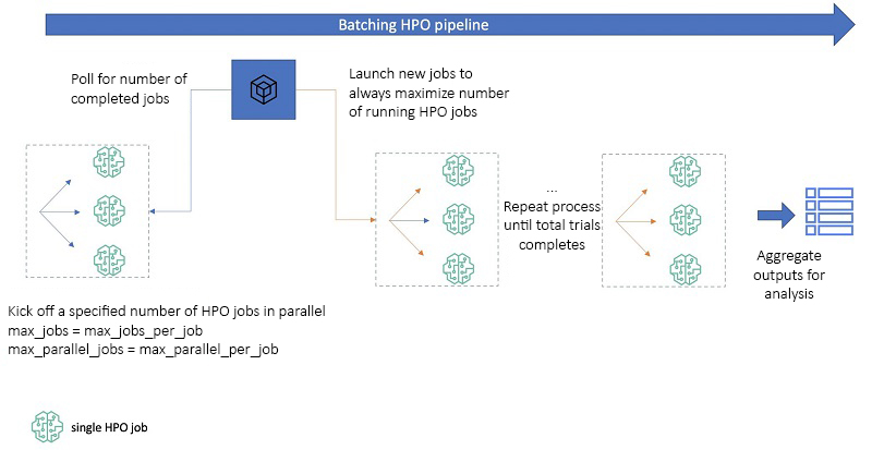
In the following code snippet, we show two ways in which you can poll the number of running jobs to achieve this. The first approach uses boto3, which is the AWS SDK for Python to poll running HPO jobs, and can be run in your notebook and is illustrated pictorially in the following diagram. This approach can primarily be used by data scientists. Whenever the number of running HPO jobs falls below a fixed number, indicated by the blue arrows in the dashed box on the left, the polling code will launch new jobs (shown in orange arrows). The second approach uses Amazon Simple Queue Service (Amazon SQS) and AWS Lambda to queue and poll SageMaker HPO jobs, allowing you to build an operational pipeline for repeatability.

Sounds complicated? No problem, the following code snippet allows you to determine the optimal strategy to minimize your overall HPO time by running as many HPO jobs in parallel as allowed. After you determine the instance type you want to use and your respective account limits for that instance, replace max_parallel_across_jobs with your value.

def bayesian_batching_cold_start(total_requested_trials, max_parallel_across_jobs=20, max_parallel_per_job=10, max_candidates_per_job = 500):
    '''Given a total number of requested trials, generates the strategy for Bayesian HPO
    The strategy is a list (batch_strat) where every element is the number of jobs to run in parallel. The sum of all elements in the list is
    the total number of HPO jobs needed to reach total_requested_trials. For example if batch_strat = [2, 2, 2, 1], means you will run a total of 7
    HPO jobs starting with 2 --> 2 ---> 2 ---> 1. 
    total_requested_trials = number of trails user wants to run.
    max_parallel_across_jobs = max number of training jobs across all trials Sagemaker runs in parallel. Limited by instance availability
    max_parallel_per_job = max number of parallel jobs to run per HPO job
    max_candidates_per_job = total number of training jobs per HPO job'''
    batch_strat = [] 
    tot_jobs_left = total_requested_trials
    max_parallel_hpo_jobs = max_parallel_across_jobs//max_parallel_per_job
    if total_requested_trials < max_parallel_hpo_jobs*max_candidates_per_job:
        batch_strat.append(total_requested_trials//max_candidates_per_job)
    else:
        while tot_jobs_left > max_parallel_hpo_jobs*max_candidates_per_job:
            batch_strat.append(max_parallel_hpo_jobs)
            tot_jobs_left -=max_parallel_hpo_jobs*max_candidates_per_job

        batch_strat.append(math.ceil((tot_jobs_left)/max_candidates_per_job))
    return math.ceil(total_requested_trials/max_candidates_per_job), max_parallel_hpo_jobs, batch_strat
                
bayesian_batching_cold_start(10000)
(20, 2, [2, 2, 2, 2, 2, 2, 2, 2, 2, 2])

After you determine how to run your jobs, consider the following code for launching a given sequence of jobs. The helper function _parallel_hpo_no_polling runs the group of parallel HPO jobs indicated by the dashed box in the preceding figure. It’s important to set the wait parameter to False when calling the tuner, because this releases the API call to allow the loop to run. The orchestration code poll_and_run polls for the number of jobs that are running at any given time. If the number of jobs falls below the user-specified maximum number of trials they want to run in parallel (max_parallel_across_jobs), the function automatically launches new jobs. Now you might be thinking,  “But these jobs can take days to run, what if I want to turn off my laptop or if I lose my session?” No problem, the code picks up where it left off and runs the remaining number of jobs by counting how many HPO jobs are remaining prefixed by the job_name_prefix you provide.

Finally, the get_best_job function aggregates the outputs in a Pandas DataFrame in ascending order of the objective metric for visualization.

# helper function to launch a desired number of "n_parallel" HPO jobs simultaneously
def _parallel_hpo_no_polling(job_name_prefix, n_parallel, inputs, max_candidates_per_job, max_parallel_per_job):
    """kicks off N_parallel Bayesian HPO jobs in parallel
    job_name_prefix: user specified prefix for job names
    n_parallel: Number of HPO jobs to start in parallel
    inputs: training and test data s3 paths
    max_candidates_per_job: number of training jobs to run in each HPO job in total
    max_parallel_per_job: number of training jobs to run in parallel in each job
    
    """
    # kick off n_parallel jobs simultaneously and returns all the job names 
    tuning_job_names = []
    for i in range(n_parallel):
        timestamp_suffix = strftime("%d-%H-%M-%S", gmtime())
        try:
            tuner = HyperparameterTuner(estimator,
                            objective_metric_name,
                            hyperparameter_ranges,
                            metric_definitions,
                            max_jobs=max_candidates_per_job,
                            max_parallel_jobs=max_parallel_per_job,
                            objective_type=objective_type
                    )
        # fit the tuner to the inputs and include it as part of experiments
            tuner.fit(inputs, 
                      job_name = f'{job_name_prefix}-{timestamp_suffix}',
                      wait=False
                     ) # set wait=False, so you can launch other jobs in parallel.
            tuning_job_names.append(tuner.latest_tuning_job.name)
            sleep(1) #this is required otherwise you will get an error for using the same tuning job name
            print(tuning_job_names)
        except Exception as e:
            sleep(5)
    return tuning_job_names

#orchestration and polling logicdef poll_and_run(job_name_prefix, inputs, max_total_candidates, max_parallel_across_jobs, max_candidates_per_job, max_parallel_per_job):
    """Polls for number of running HPO jobs. If less than max_parallel , starts a new one. 
    job_name_prefix: the name prefix to give all your training jobs
    max_total_candidates: how many total trails to run across all HPO jobs
    max_candidates_per_job: how many total trails to run for 1 HPO job 
    max_parallel_per_job: how many trials to run in parallel for a given HPO job (fixed to 10 without limit increases). 
    max_parallel_across_jobs: how many concurrent trials to run in parallel across all HPO jobs
    """
    #get how many jobs to run in total and concurrently
    max_num, max_parallel, _ = bayesian_batching_cold_start(max_total_candidates, 
                                                            max_parallel_across_jobs=max_parallel_across_jobs,
                                                            max_parallel_per_job=max_parallel_per_job,
                                                            max_candidates_per_job = max_candidates_per_job
                                                           )
    
    # continuously polls for running jobs -- if they are less than the required number, then launches a new one. 

    all_jobs = sm.list_hyper_parameter_tuning_jobs(SortBy='CreationTime', SortOrder='Descending', 
                                                       NameContains=job_name_prefix,
                                                        MaxResults = 100)['HyperParameterTuningJobSummaries']
    all_jobs = [i['HyperParameterTuningJobName'] for i in all_jobs]

    if len(all_jobs)==0:
        print(f"Starting a set of HPO jobs with the prefix {job_name_prefix} ...")
        num_left = max_num
        #kick off the first set of jobs
        all_jobs += _parallel_hpo_no_polling(job_name_prefix, min(max_parallel, num_left), inputs, max_candidates_per_job, max_parallel_per_job)
        
    else:
        print("Continuing where you left off...")
        response_list = [sm.describe_hyper_parameter_tuning_job(HyperParameterTuningJobName=i)['HyperParameterTuningJobStatus']
                         for i in all_jobs]
        print(f"Already completed jobs = {response_list.count('Completed')}")
        num_left = max_num - response_list.count("Completed")
        print(f"Number of jobs left to complete = {max(num_left, 0)}")
    
    while num_left >0:
        response_list = [sm.describe_hyper_parameter_tuning_job(HyperParameterTuningJobName=i)['HyperParameterTuningJobStatus']
                         for i in all_jobs]
        running_jobs = response_list.count("InProgress") # look for the jobs that are running. 
        print(f"number of completed jobs = {response_list.count('Completed')}")
        sleep(10)
        if running_jobs < max_parallel and len(all_jobs) < max_num:
            all_jobs += _parallel_hpo_no_polling(job_name_prefix, min(max_parallel-running_jobs, num_left), inputs, max_candidates_per_job, max_parallel_per_job)
        num_left = max_num - response_list.count("Completed")
                
    return all_jobs
# Aggregate the results from all the HPO jobs based on the custom metric specified
def get_best_job(all_jobs_list):
    """Get the best job from the list of all the jobs completed.
    Objective is to maximize a particular value such as AUC or F1 score"""
    df = pd.DataFrame()
    for job in all_jobs_list:
        tuner = sagemaker.HyperparameterTuningJobAnalytics(job)
        full_df = tuner.dataframe()
        tuning_job_result = sm.describe_hyper_parameter_tuning_job(HyperParameterTuningJobName=job)
        is_maximize = (tuning_job_result['HyperParameterTuningJobConfig']['HyperParameterTuningJobObjective']['Type'] == 'Maximize')
        if len(full_df) > 0:
            df = pd.concat([df, full_df[full_df['FinalObjectiveValue'] < float('inf')]])
    if len(df) > 0:
        df = df.sort_values('FinalObjectiveValue', ascending=is_maximize)
        print("Number of training jobs with valid objective: %d" % len(df))
        print({"lowest":min(df['FinalObjectiveValue']),"highest": max(df['FinalObjectiveValue'])})
        pd.set_option('display.max_colwidth', -1)  # Don't truncate TrainingJobName
        return df
    else:
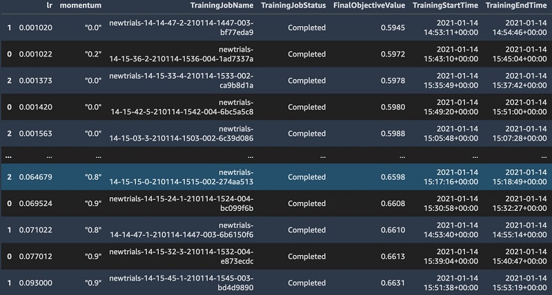
        print("No training jobs have reported valid results yet.")

Now, we can test this out by running a total of 260 trials, and request that the code run 20 trials in parallel at all times:

alljobs = poll_and_run('newtrials', inputs, max_total_candidates=260, max_parallel_across_jobs = 20, max_candidates_per_job=4, max_parallel_per_job=2)

After the jobs are complete, we can look at all the outputs (see the following screenshot).

The above code will allow you to run HPO jobs in parallel up to the allowed limit of 100 concurrent HPO jobs.

Parallelizing HPO jobs with warm start

Now suppose you want to run a warm start job, where the result of a prior job is used as input to the next job. Warm start is particularly useful if you have already determined a set of hyperparameters that produce a good model but now have new data. Another use case for warm start is when a single HPO job can take a long time, particularly for deep learning workloads. In that case, you may want to use the outputs of the prior job to launch the next one. For our use case, that could occur when you get a batch of new monthly or quarterly default data. For more information about SageMaker HPO with warm start, see Run a Warm Start Hyperparameter Tuning Job.

The crucial difference between warm and cold start is the naturally sequential nature of warm start. Again, suppose we want to launch 10,000 jobs with warm start. This time, we only launch a single HPO job with the maximally allowed max_jobs parameter, wait for its completion, and launch the next job with this job as parent. We repeat the process until the total desired number of jobs is reached. We can achieve this with the following code:

def large_scale_hpo_warmstart(job_name_prefix, inputs, max_total_trials,  max_parallel_per_job, max_trials_per_hpo_job=250):
    """Kicks off sequential HPO jobs with warmstart. 
    job_name_prefix: user defined prefix to name your HPO jobs. HPO will add a timestamp
    inputs: locations of train and test datasets in S3 provided as a dict
    max_total_trials: total number of trials you want to run
    max_trials_per_hpo_job: Fixed at 250 unless you want fewer.
    max_parallel_per_job: max trails to run in parallel per HPO job"""
    
    if max_trials_per_hpo_job >250:
        raise ValueError('Please select a value less than or equal to 250 for max_trials_per_hpo_job')
    
    base_hpo_job_name = job_name_prefix
    timestamp_suffix = strftime("%d-%H-%M-%S", gmtime())
    tuning_job_name = lambda i : f"{base_hpo_job_name}-{timestamp_suffix}-{i}"
    current_jobs_completed = 0
    job_names_list = []
    while current_jobs_completed < max_total_trials:
        jobs_to_launch = min(max_total_trials - current_jobs_completed, max_trials_per_hpo_job)

        hpo_job_config = dict(
            estimator=estimator,
            objective_metric_name=objective_metric_name,
            metric_definitions=metric_definitions,
            hyperparameter_ranges=hyperparameter_ranges,
            max_jobs=jobs_to_launch,
            strategy="Bayesian",
            objective_type=objective_type,
            max_parallel_jobs=max_parallel_per_job,
        )

        if current_jobs_completed > 0:
            parent_tuning_job_name = tuning_job_name(current_jobs_completed)
            warm_start_config = WarmStartConfig(
                WarmStartTypes.IDENTICAL_DATA_AND_ALGORITHM,
                parents={parent_tuning_job_name}
            )
            hpo_job_config.update(dict(
                base_tuning_job_name=parent_tuning_job_name,
                warm_start_config=warm_start_config
            ))

        tuner = HyperparameterTuner(**hpo_job_config)
        tuner.fit(
            inputs,
            job_name=tuning_job_name(current_jobs_completed + jobs_to_launch),
            logs=True,
        )
        tuner.wait()
        job_names_list.append(tuner.latest_tuning_job.name)
        current_jobs_completed += jobs_to_launch
    return job_names_list

After the jobs run, again use the get_best_job function to aggregate the findings.

Using other HPO tools with SageMaker

SageMaker offers the flexibility to use other HPO tools such as the ones discussed earlier to run your HPO jobs by removing the undifferentiated heavy lifting of managing the underlying infrastructure. For example, a popular open-source HPO tool is Ray Tune [2], which is a Python library for large-scale HPO that supports most of the popular frameworks such as XGBoost, MXNet, PyTorch, and TensorFlow. Ray integrates with popular search algorithms such as Bayesian, HyperOpt, and SigOpt, combined with state-of-the-art schedulers such as Hyperband or ASHA.

To use Ray with PyTorch, you first need to include ray[tune] and tabulate to your requirements.txt file in your code folder containing your training script. Provide the code folder into the SageMaker PyTorch estimator as follows:

from sagemaker.pytorch import PyTorch

estimator = PyTorch(entry_point="train_ray_cpu.py", #put requirements.txt file to install ray
                    role=role,
                    source_dir='./code',
                    framework_version='1.6.0',
                    py_version='py3',
                    output_path = f's3://{bucket}/{prefix}/output',
                    instance_count=1,
                    instance_type='ml.m5.xlarge',
                    sagemaker_session=sagemaker_session,
                    hyperparameters={
                        'epochs': 7,
                        'backend': 'gloo' # gloo for CPU and nccl for GPU
                    },
                   disable_profiler=True)

inputs ={'training': train_s3,
         'testing':test_s3}

estimator.fit(inputs, wait=True)

Your training script needs to be modified to output your custom metrics to the Ray report generator, as shown in the following code. This allows your training job to communicate with Ray. Here we use the ASHA scheduler to implement early stopping:

# additional imports
from ray.tune import CLIReporter
from ray.tune.schedulers import ASHAScheduler

# modify test function to output to ray tune report.
def test(model, test_loader, device):
    # same as test function above with 1 line of code added to enable communication 
    # with tune.
    tune.report(loss=test_loss, accuracy=correct / (len(target)*i), f1score=f1score, roc=roc)

You also need to checkpoint your model at regular intervals:

for epoch in range(1, args.epochs + 1):
        model.train()
        for batch_idx, (data, target) in enumerate(train_loader, 1):
            data, target = data.to(device), target.to(device)
            optimizer.zero_grad()
            output = model(data)
            loss = F.nll_loss(output, target.squeeze())
            loss.backward()
     
            optimizer.step()
            if batch_idx % args.log_interval == 0:
                logger.info("Train Epoch: {} [{}/{} ({:.0f}%)] Loss: {:.6f}".format(
                    epoch, batch_idx * len(data), len(train_loader.sampler),
                    100. * batch_idx / len(train_loader), loss.item()))
        # have your test function publish metrics to tune.report
        test(model, test_loader, device)
        # checkpoint your model
        with tune.checkpoint_dir(epoch) as checkpoint_dir: # modified to store checkpoint after every epoch.
                path = os.path.join(checkpoint_dir, "checkpoint")
                torch.save((model.state_dict(), optimizer.state_dict()), path)

Finally, you need to wrap the training script in a custom main function that sets up the hyperparameters such as the learning rate, the size of the first and second hidden layers, and any additional hyperparameters you want to iterate over. You also need to use a scheduler, such as the ASHA scheduler we use here, for single- and multi-node GPU training. We use the default tuning algorithm Variant Generation, which supports both random (shown in the following code) and grid search, depending on the config parameter used.

def main(args):
    config = {
        "l1": tune.sample_from(lambda _: 2**np.random.randint(2, 9)),
        "l2": tune.sample_from(lambda _: 2**np.random.randint(2, 9)),
        "lr": tune.loguniform(1e-4, 1e-1)
    }
    scheduler = ASHAScheduler(
        metric="loss",
        mode="min",
        max_t=args.epochs,
        grace_period=1,
        reduction_factor=2)
    reporter = CLIReporter(
        metric_columns=["loss","training_iteration", "roc"])
    
    # run the HPO job by calling train
    print("Starting training ....")
    result = tune.run(
        partial(train_ray, args=args),
        resources_per_trial={"cpu": args.num_cpus, "gpu": args.num_gpus},
        config=config,
        num_samples=args.num_samples,
        scheduler=scheduler,
        progress_reporter=reporter)

The output of the job looks like the following screenshot.

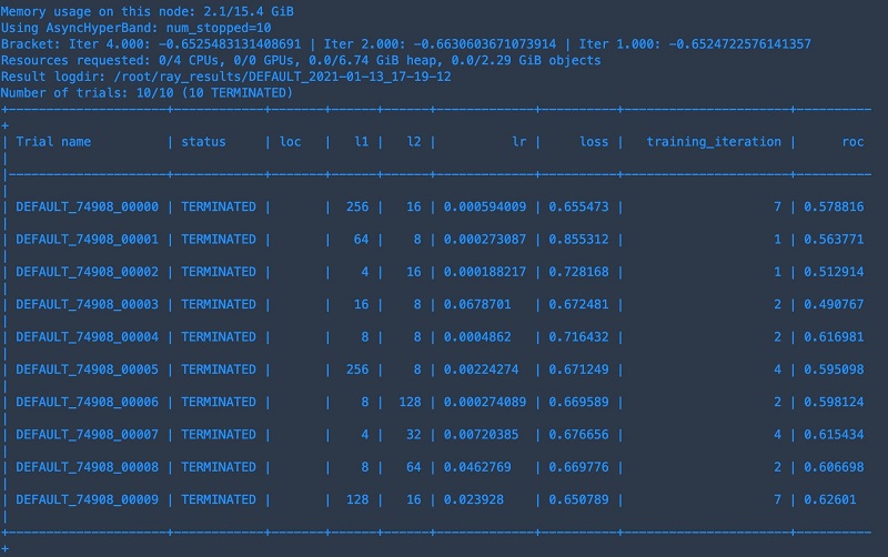
Ray Tune automatically ends poorly performing jobs while letting the better-performing jobs run longer, optimizing your total HPO times. In this case, the best-performing job ran all full 7 epochs, whereas other hyperparameter choices were stopped early. To learn more about how early stopping works with SageMaker HPO see here.

Queuing HPO jobs with Amazon SQS

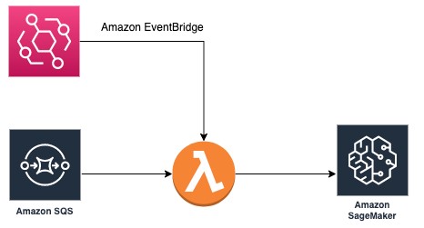
When multiple data scientists create HPO jobs in the same account at the same time, the limit of 100 concurrent HPO jobs per account might be reached. In this case, we can use Amazon SQS to create an HPO job queue. Each HPO job request is represented as a message and submitted to an SQS queue. Each message contains hyperparameters and tunable hyperparameter ranges in the message body. A Lambda function is also created. The function first checks the number of HPO jobs in progress. If the 100 concurrent HPO jobs limit isn’t reached, it retrieves messages from the SQS queue and creates HPO jobs as stipulated in the message. The function is triggered by Amazon EventBridge events at a regular interval (for example, every 10 minutes). The simple architecture is shown as follows.

To build this architecture, we first create an SQS queue and note the URL. In the Lambda function, we use the following code to return the number of HPO jobs in progress:

sm_client = boto3.client('sagemaker')

def check_hpo_jobs():
    response = sm_client.list_hyper_parameter_tuning_jobs(
    MaxResults=HPO_LIMIT,
    StatusEquals='InProgress')
    return len(list(response["HyperParameterTuningJobSummaries"]))

If the number of HPO jobs in progress is greater than or equal to the limit of 100 concurrent HPO jobs (for current limits, see Amazon SageMaker endpoints and quotas), the Lambda function returns 200 status and exits. If the limit isn’t reached, the function calculates the number of HPO jobs available for creation and retrieves the same number of messages from the SQS queue. Then the Lambda function extracts hyperparameter ranges and other data fields for creating HPO jobs. If the HPO job is created successfully, the corresponding message is deleted from the SQS queue. See the following code:

def lambda_handler(event, context):
    
    # first: check HPO jobs in progress
    hpo_in_progress = check_hpo_jobs()
    
    if hpo_in_progress >= HPO_LIMIT:
        return {
        'statusCode': 200,
        'body': json.dumps('HPO concurrent jobs limit reached')
    }
    else:
        hpo_capacity = HPO_LIMIT - hpo_in_progress
        container = image_uris.retrieve("xgboost", region, "0.90-2")
        train_input = TrainingInput(f"s3://{bucket}/{key_prefix}/train/train.csv", content_type="text/csv")
        validation_input = TrainingInput(f"s3://{bucket}/{key_prefix}/validation/validation.csv", content_type="text/csv")
      
        while hpo_capacity > 0:
            sqs_response = sqs.receive_message(QueueUrl = queue_url)
            if 'Messages' in sqs_response.keys():
                msgs = sqs_response['Messages']
                for msg in msgs:
                    try:
                        hp_in_msg = json.loads(msg['Body'])['hyperparameter_ranges']
                        create_hpo(container,train_input,validation_input,hp_in_msg)
                        response = sqs.delete_message(QueueUrl=queue_url,ReceiptHandle=msg['ReceiptHandle'])
                        hpo_capacity = hpo_capacity-1
                        if hpo_capacity == 0: 
                            break
                    except :
                        return ("error occurred for message {}".format(msg['Body']))
            else:
                return {'statusCode': 200, 'body': json.dumps('Queue is empty')}
    
        return {'statusCode': 200,  'body': json.dumps('Lambda completes')}

After your Lambda function is created, you can add triggers with the following steps:

1. On the Lambda console, choose your function.
2. On the Configuration page, choose Add trigger.
3. Select EventBridge (CloudWatch Events).
4. Choose Create a new rule.
5. Enter a name for your rule.
6. Select Schedule expression.
7. Set the rate to 10 minutes.
8. Choose Add.

This rule triggers our Lambda function every 10 minutes.

When this is complete, you can test it out by sending messages to the SQS queue with your HPO job configuration in the message body. The code and notebook for this architecture is on our GitHub repo. See the following code:

response = sqs.send_message(
    QueueUrl=queue_url,
    DelaySeconds=1,
    MessageBody=(
        '{"hyperparameter_ranges":{
            "<hyperparamter1>":<range>,
            "hyperparamter2":<range>} }'
        )
    )

Conclusions

ML engineers often need to search through a large hyperparameter space to find the best-performing model for their use case. For complex deep learning models, where individual training jobs can be quite time consuming, this can be a cumbersome process that can often take weeks or months of developer time.

In this post, we discussed how you can maximize the number of tuning jobs you can launch in parallel with SageMaker, which reduces the total time it takes to run HPO with custom user-specified objective metrics. We first discussed a Jupyter notebook based approach that can be used by individual data scientists for research and experimentation workflows. We also demonstrated how to use an SQS queue to allow teams of data scientists to submit more jobs. SageMaker is a highly flexible platform, allowing you to bring your own HPO tool, which we illustrated using the popular open-source tool Ray Tune.

To learn more about bringing other algorithms such as genetic algorithms to SageMaker HPO, see Bring your own hyperparameter optimization algorithm on Amazon SageMaker.

References

About the Authors

Iaroslav Shcherbatyi is a Machine Learning Engineer at Amazon Web Services. His work is centered around improvements to the Amazon SageMaker platform and helping customers best use its features. In his spare time, he likes to catch up on recent research in ML and do outdoor sports such as ice skating or hiking.

Enrico Sartorello is a Sr. Software Development Engineer at Amazon Web Services. He helps customers adopt machine learning solutions that fit their needs by developing new functionalities for Amazon SageMaker. In his spare time, he passionately follows his soccer team and likes to improve his cooking skills.

Tushar Saxena is a Principal Product Manager at Amazon, with the mission to grow AWS’ file storage business. Prior to Amazon, he led telecom infrastructure business units at two companies, and played a central role in launching Verizon’s fiber broadband service. He started his career as a researcher at GE R&D and BBN, working in computer vision, Internet networks, and video streaming.

Stefan Natu is a Sr. Machine Learning Specialist at Amazon Web Services. He is focused on helping financial services customers build end-to-end machine learning solutions on AWS. In his spare time, he enjoys reading machine learning blogs, playing the guitar, and exploring the food scene in New York City.

Qingwei Li is a Machine Learning Specialist at Amazon Web Services. He received his PhD in Operations Research after he broke his advisor’s research grant account and failed to deliver the Nobel Prize he promised. Currently, he helps customers in the financial service and insurance industry build machine learning solutions on AWS. In his spare time, he likes reading and teaching.

Read More

Personal protective equipment (PPE) such as face covers (face mask), hand covers (gloves), and head covers (helmet) are essential for many businesses. For example, helmets are required at construction sites for employee safety, and gloves and face masks are required in the restaurant industry for hygienic operations. In the current COVID-19 pandemic environment, PPE compliance has also become important as face masks are mandated by many businesses. In this post, we demonstrate how you can deploy a solution to automatically check face mask compliance on your business premises and extract actionable insights using the Amazon Rekognition DetectProtectiveEquipment API.

This solution has been developed by AWS Professional Services to help customers that rely heavily on on-site presence of customers or employees to support their safety. Our team built the following architecture to automate PPE detection by consuming the customer’s camera video feeds. This solution enabled a large sports entertainment customer to take timely action to ensure people who are on the premises comply with face mask requirements. The architecture is designed to take raw camera feeds for model inference and pass the model output to an analytic dashboard for further analysis. As of this writing, it’s successfully deployed at a customer site with multiple production cameras.

Let’s walk through the solution in detail and discuss the scalability and security of the application.

Solution overview

The PPE detection solution architecture is an end-to-end pipeline consisting of three components:

• Video ingestion pipeline – Ensures you receive on-demand video feeds from camera and preprocesses the feeds to break them into frames. Finally, it saves the frames in an Amazon Simple Storage Service (Amazon S3) bucket for ML model inference.
• Machine learning inference pipeline – Demonstrates how the machine learning (ML) model processes the frames as soon as they arrive at the S3 bucket. The model outputs are stored back in the S3 bucket for further visualization.
• Model interaction pipeline – Used for visualizing the model outputs. The model outputs feed into Amazon QuickSight, which you can use to analyze the data based on the camera details, day, and time of day.

The following diagram illustrates this architecture (click to expand).

We now discuss each section in detail.

Video ingestion pipeline

The following diagram shows the architecture of the video ingestion pipeline.

The video ingestion pipeline begins at a gateway located on premises at the customer location. The gateway is a Linux machine with access to RTSP streams on the cameras. Installed on the gateway is the open-source GStreamer framework and AWS-provided Amazon Kinesis Video Streams GStreamer plugin. For additional information on setting up a gateway with the tools needed to stream video to AWS, see Example: Kinesis Video Streams Producer SDK GStreamer Plugin.

The gateway continuously publishes live video to a Kinesis video stream, which acts like a buffer while AWS Fargate tasks read video fragments for further processing. To accommodate customer-specific requirements around the location of cameras that periodically come online and the time of day when streaming processing is needed, we developed a cost-effective and low-operational overhead consumer pipeline with automatic scaling. This avoids manually starting and stopping processing tasks when a camera comes online or goes dark.

Consuming from Kinesis Video Streams is accomplished via an AWS Fargate task running on Amazon Elastic Container Service (Amazon ECS). Fargate is a serverless compute engine that removes the need to provision and manage servers, and you pay for compute resources only when necessary. Processing periodic camera streams is an ideal use case for a Fargate task, which was developed to automatically end when no video data is available on a stream. Additionally, we built the framework to automatically start tasks using a combination of Amazon CloudWatch alarms, AWS Lambda, and checkpointing tables in Amazon DynamoDB. This ensures that the processing always continues from the video segment where the streaming data was paused.

The Fargate task consumes from the Kinesis Video Streams GetMedia API to obtain real-time, low-latency access to individual video fragments and combines them into video clips of 30 seconds or more. The video clips are then converted from MKV to an MP4 container and resampled to 1 frame per second (FPS) to extract an image from each second of video. Finally, the processed video clips and images are copied into an S3 bucket to feed the ML inference pipeline.

ML inference pipeline

The following diagram illustrates the architecture of the ML pipeline.

The ML pipeline is architected to be automatically triggered when new data lands in the S3 bucket, and it utilizes a new deep learning-based computer vision model tailored for PPE detection in Amazon Rekognition. As soon as the S3 bucket receives a new video or image object, it generates and delivers an event notification to an Amazon Simple Queue Service (Amazon SQS) queue, where each queue item triggers a Lambda invocation. Each Lambda invocation calls the Amazon Rekognition DetectProtectiveEquipment API to generate model inference and delivers the result back to Amazon S3 through Amazon Kinesis Data Firehose.

The Amazon Rekognition PPE API detects several types of equipment, including hand covers (gloves), face covers (face masks), and head covers (helmets). For our use case, the customer was focused on detecting face masks. The computer vision model in Amazon Rekognition first detects if people are in a given image, and then detects face masks. Based on the location of the face mask on a face, if a person is wearing a face mask not covering their nose or mouth, the service will assign a noncompliant label. When the model can’t detect a face due to image quality, such as when the region of interest (face) is too small, it labels that region as unknown. For each image, the Amazon Rekognition API returns the number of compliant, noncompliant, and unknowns, which are used to calculate meaningful metrics for end users. The following table lists the metrics.

We use the following formulas to calculate these metrics:

• Total number of noncompliant = Total number of detected faces not wearing face cover in the frame
• Total number of compliant = Total number of detected faces wearing face cover in the frame
• Total number of unknowns = Total number of people for which a face cover or face can’t be detected in the frame
• Total number of detected faces = Total number of noncompliant + Total number of compliant
• Total number of detected people = Total number of unknowns + Total number of detected faces
• Mask noncompliant per frame = Total number of noncompliant in the frame

Preprocessing for crowded images and images of very small size

Amazon Rekognition PPE detection supports up to 15 people per image. To support images where more than 15 people are present, we fragment the image into smaller tiles and process them via Amazon Rekognition. Also, PPE detection requires a minimum face size of 40×40 pixels for an image with 1920×1080 pixels. If the image is too small, we interpolate it before performing inference. For more information about size limits, see Guidelines and Quotas in Amazon Rekognition.

Model interaction pipeline

Finally, we can visualize the calculated metrics in QuickSight. QuickSight is a cloud-native and serverless business intelligence tool that enables straightforward creation of interactive visualizations. For more information about setting up a dashboard, see Getting Started with Data Analysis in Amazon QuickSight.

As shown in the following dashboard, end users can configure and display the top priority statistics at the top of the dashboard, such as total count of noncompliant, seating area total count of noncompliant, and front entrance total count of noncompliant. In addition, end users can interact with the line chart to dive deep into the mask-wearing noncompliant patterns. The bottom chart shows such statistics of the eight cameras over time.

You can create additional visualizations according to your business needs. For more information, see Working with Visual Types in Amazon QuickSight.

Code template

This section contains the code template to help you get started in deploying this solution into your AWS account. This is an AWS Serverless Application Model (AWS SAM) project and requires you to have the AWS Command Line Interface (AWS CLI) and AWS SAM CLI set up in your system.

To build and deploy the AWS CloudFormation stack, complete the following steps:

1. Install the AWS CLI and configure your AWS CLI credentials.
2. Install the AWS SAM CLI using these instructions.
3. Download the Ppe-detection-ml-pipeline.zip
4. Unzip the contents of the .zip file and navigate to the root of the project.
5. Build the project – This will package the Lambda functions. Note: Python 3.8 and pip are required for this deployment.

   sam build

6. Deploy the CloudFormation stack in your AWS account

   sam deploy --guided

Choose an appropriate AWS region to deploy the stack. Use the defaults for all other prompts.
Note: Use sam deploy for subsequent stack updates.

Note: The Rekognition PPE API needs the following SDK versions: boto3 >= 1.15.17 and botocore >=1.18.17. Currently, the AWS Lambda Python 3.8 runtime does not support the preceding versions (see documentation). A layer has been added to the Lambda function in template to support the required SDK versions. We will update this post and the code template after the updated SDK is natively supported by the Python 3.8 runtime.

We use Amazon S3 as a data lake to store the images coming out of the video ingestion pipeline after it splits the original camera feeds into 1 FPS images. The S3 data lake bucket folder structure, which organizes the collected image and camera metadata along with the model responses.

After deploying the stack, create the input folder inside the S3 bucket. The input prefix can contain multiple folders, which helps in organizing the results by camera source. To test the pipeline, upload a .jpg containing people and faces to input/[camera_id]/ folder in the S3 bucket. The camera_id can be any arbitrary name. The output and error prefixes are created automatically when the PPE detection job is triggered. The output prefix contains model inference outputs. The error prefix contains records of jobs that failed to run. Make sure you have a similar folder structure in the deployed S3 bucket for the code to work correctly.

S3 DataLake Bucket
-- input/
---- [camera_id]/ 
-- output/
---- ppe/
------ [YYYY]/[MM]/[DD]/
-- error/
---- ppe/

For example, this sample image is uploaded to the S3 Bucket location: input/CAMERA01/. After Amazon Kinesis Data Firehose delivers the event to Amazon S3, the output/ prefix will contain a file with a JSON record indicating the PPE compliant status of each individual.

{
  "CameraID": "CAMERA01",
  "Bucket": "ppe-detection-blog-post-datalakes3bucket-abc123abc123",
  "Key": "input/CAMERA01/ppe_sample_image.jpg",
  "RekResult": "{"0": "compliant", "1": "compliant", "2": "compliant", "3": "compliant"}",
  "FaceCoverNonCompliant": 0,
  "FaceCoverNonCompliantPercentage": 0,
  "detectedFaceRate": 100
}

The provided AWS SAM project creates the resources, roles, and necessary configuration of the pipeline. Note that the IAM roles deployed are very permissive and should be restricted in production environments.

Conclusion

In this post, we showed how we take a live camera feed as input to build a video ingestion pipeline and prepare the data for ML inference. Next we demonstrated a scalable solution to perform PPE detection using the Amazon Rekognition API. Then we discussed how to visualize the model output results on a QuickSight dashboard for building meaningful dashboards for your safety compliance guidelines. Finally, we provided an AWS SAM project of the ML pipeline if you want to deploy this in your own AWS account.

We also demonstrated how the AWS Professional Services team can help customers with the implementation and deployment of an end-to-end architecture for detecting PPE at scale using Amazon Rekognition’s new PPE detection feature. For additional information, see Automatically detecting personal protective equipment on persons in images using Amazon Rekognition to learn more about the new PPE detection API, insight into model outputs, and different ways to deploy a PPE solution for your own camera and networking requirements.

AWS Professional Services can help customize and implement the PPE detection solution based on your organization’s requirements. To learn more about how we can help, please connect with us with the help of your account manager.

About the Authors

Pranati Sahu is a Data Scientist at AWS Professional Services and Amazon ML Solutions Lab team. She has an MS in Operations Research from Arizona State University, Tempe and has worked on machine learning problems across industries including social media, consumer hardware, and retail. In her current role, she is working with customers to solve some of the industry’s complex machine learning use cases on AWS.

Surya Dulla is an Associate Cloud Developer at AWS Professional Services. She has an MS in Computer Science from Towson University, Maryland. She has experience in developing full stack applications, microservices in health care and financial industry. In her current role, she focuses on delivering best operational solutions for enterprises using AWS suite of developer tools.

Rohit Rangnekar is a Principal IoT Architect with AWS Professional Services based in the San Francisco Bay Area. He has an MS in Electrical Engineering from Virginia Tech and has architected and implemented data & analytics, AI/ML, and IoT platforms globally. Rohit has a background in software engineering and IoT edge solutions which he leverages to drive business outcomes in healthcare, space and telecom, semiconductors and energy verticals among others.

Taihua (Ray) Li is a data scientist with AWS Professional Services. He holds a M.S. in Predictive Analytics degree from DePaul University and has several years of experience building artificial intelligence powered applications for non-profit and enterprise organizations. At AWS, Ray helps customers to unlock business potentials and to drive actionable outcomes with machine learning. Outside of work, he enjoys fitness classes, biking, and traveling.

Han Man is a Data Scientist with AWS Professional Services. He has a PhD in engineering from Northwestern University and has several years of experience as a management consultant advising clients across many industries. Today he is passionately working with customers to develop and implement machine learning, deep learning, & AI solutions on AWS. He enjoys playing basketball in his spare time and taking his bulldog, Truffle, to the beach.

Jin Fei is a Senior Data Scientist with AWS Professional Services. He has a PhD in computer science in the area of computer vision and image analysis from University of Houston. He has worked as researchers and consultants in different industries including energy, manufacture, health science and finance. Other than providing machine learning and deep learning solutions to customers, his specialties also include IoT, software engineering and architectural design. He enjoys reading, photography, and swimming.

Kareem Williams is a data scientist with Amazon Research. He holds a M.S. in Data Science from Southern Methodist University and has several years of experience solving challenging business problems with ML for SMB and Enterprise organizations. Currently, Kareem is working on leveraging AI to build a more diverse and inclusive workspace at Amazon. In his spare time he enjoys soccer, hikes, and spending time with his family.

Read More

With the rapid growth of object detection techniques, several frameworks with packaged pre-trained models have been developed to provide users easy access to transfer learning. For example, GluonCV, Detectron2, and the TensorFlow Object Detection API are three popular computer vision frameworks with pre-trained models.

In this post, we use Amazon SageMaker to build, train, and deploy an EfficientDet model using the TensorFlow Object Detection API. It’s built on top of TensorFlow 2, which makes it easy to construct, train, and deploy object detection models.

It also provides the TensorFlow 2 Detection Model Zoo, which is a collection of pre-trained detection models we can use to accelerate our endeavor.

SageMaker is a fully managed service that provides developers and data scientists the ability to build, train, and deploy ML models quickly. SageMaker removes the heavy lifting from each step of the ML process to make it easier to develop high-quality models.

Walkthrough overview

This post demonstrates how to do the following:

• Label images using SageMaker Ground Truth
• Generate the dataset TFRecords and label map using SageMaker Processing
• Fine-tune an EfficientDet model with TensorFlow 2 on SageMaker
• Monitor your model training with TensorBoard and SageMaker Debugger
• Deploy your model on a SageMaker endpoint and visualize predictions

Prerequisites

If you want to try out each step yourself, make sure that you have the following in place:

• An AWS account
• An Amazon Simple Storage Service (Amazon S3) bucket
• A running SageMaker notebook instance
• The following GitHub repository cloned to the SageMaker notebook instance

The code repo contains the following folders with step-by-step walkthrough via notebooks.

Preparing the data

You can follow this section by running the cells in this notebook.

The dataset

In this post, we use a dataset from iNaturalist.org and train a model to recognize bees from RGB images.

This dataset contains 500 images of bees that have been uploaded by iNaturalist users for the purposes of recording the observation and identification. We only use images that users have licensed under a CC0 license.

We placed the dataset in Amazon S3 in a single .zip archive that you can download or by following instructions in the prepare_data.ipynb notebook in your instance.

The archive contains 500 .jpg image files, and an output.manifest file, which we explain later in the post. We also have 10 test images in the 3_predict/test_images notebook folder that we use to visualize our model predictions.

Labeling images using SageMaker Ground Truth

To train an ML model, you need large, high-quality, labeled datasets. Labeling thousands of images can become tedious and time-consuming. Thankfully, Ground Truth makes it easy to crowdsource this task. Ground Truth offers easy access to public and private human labelers for annotating datasets. It provides built-in workflows and interfaces for common labeling tasks, including drawing bounding boxes for object detection.

You can now move on to creating labeling jobs in Ground Truth. In this post, we don’t cover each step in creating a labeling job. It’s already covered in detail in the post Amazon SageMaker Ground Truth – Build Highly Accurate Datasets and Reduce Labeling Costs by up to 70%.

For our dataset, we follow the recommended workflow from the post Create high-quality instructions for Amazon SageMaker Ground Truth labeling jobs to create our labeling instructions for the labeler.

The following screenshot shows an example of a labeling job configuration in Ground Truth.

At the end of a labeling job, Ground Truth saves an output manifest file in Amazon S3, where each line corresponds to a single image and its labeled bounding boxes, alongside some metadata. See the following code:

{"source-ref":"s3://sagemaker-remars/datasets/na-bees/500/10006450.jpg","bees-500":{"annotations":[{"class_id":0,"width":95.39999999999998,"top":256.2,"height":86.80000000000001,"left":177}],"image_size":[{"width":500,"depth":3,"height":500}]},"bees-500-metadata":{"job-name":"labeling-job/bees-500","class-map":{"0":"bee"},"human-annotated":"yes","objects":[{"confidence":0.75}],"creation-date":"2019-05-16T00:15:58.914553","type":"groundtruth/object-detection"}}
{"source-ref":"s3://sagemaker-remars/datasets/na-bees/500/10022723.jpg","bees-500":{"annotations":[{"class_id":0,"width":93.8,"top":228.8,"height":135,"left":126.8}],"image_size":[{"width":375,"depth":3,"height":500}]},"bees-500-metadata":{"job-name":"labeling-job/bees-500","class-map":{"0":"bee"},"human-annotated":"yes","objects":[{"confidence":0.82}],"creation-date":"2019-05-16T00:41:33.384412","type":"groundtruth/object-detection"}}
{"source-ref":"s3://sagemaker-remars/datasets/na-bees/500/10059108.jpg","bees-500":{"annotations":[{"class_id":0,"width":157.39999999999998,"top":188.60000000000002,"height":131.2,"left":110.8}],"image_size":[{"width":375,"depth":3,"height":500}]},"bees-500-metadata":{"job-name":"labeling-job/bees-500","class-map":{"0":"bee"},"human-annotated":"yes","objects":[{"confidence":0.8}],"creation-date":"2019-05-16T00:57:28.636681","type":"groundtruth/object-detection"}}
{"source-ref":"s3://sagemaker-remars/datasets/na-bees/500/10250726.jpg","bees-500":{"annotations":[{"class_id":0,"width":77.20000000000002,"top":204,"height":94.4,"left":79.6}],"image_size":[{"width":375,"depth":3,"height":500}]},"bees-500-metadata":{"job-name":"labeling-job/bees-500","class-map":{"0":"bee"},"human-annotated":"yes","objects":[{"confidence":0.81}],"creation-date":"2019-05-16T00:34:21.300882","type":"groundtruth/object-detection"}}

For your convenience, we previously completed a labeling job called bees-500 and included the augmented manifest file output.manifest in the dataset.zip archive. In the provided notebook, we upload this dataset to the default S3 bucket before data preparation.

Generating TFRecords and the dataset label map

To use our dataset in the TensorFlow Object Detection API, we must first combine its images and labels and convert them into the TFRecord file format. The TFRecord format is a simple format for storing a sequence of binary records, which helps in data reading and processing efficiency. We also need to generate a label map, which defines the mapping between a class ID and a class name.

In the provided preprocessing notebook, we build a custom SageMaker Processing job with our own processing container. We first build a Docker container with the necessary TensorFlow image, Python libraries, and code to run those steps and push it to an Amazon Elastic Container Registry (Amazon ECR) repository. We then launch a processing job, which runs the pushed container and prepares the data for training. See the following code:

data_processor = Processor(role=role, 
                           image_uri=container, 
                           instance_count=1, 
                           instance_type='ml.m5.xlarge',
                           volume_size_in_gb=30, 
                           max_runtime_in_seconds=1200,
                           base_job_name='tf2-object-detection')

input_folder = '/opt/ml/processing/input'
ground_truth_manifest = '/opt/ml/processing/input/output.manifest'
label_map = '{"0": "bee"}' # each class ID should map to the human readable equivalent
output_folder = '/opt/ml/processing/output'

data_processor.run(
    arguments= [
        f'--input={input_folder}',
        f'--ground_truth_manifest={ground_truth_manifest}',
        f'--label_map={label_map}',
        f'--output={output_folder}'
    ],
    inputs = [
        ProcessingInput(
            input_name='input',
            source=s3_input,
            destination=input_folder
        )
    ],
    outputs= [
        ProcessingOutput(
            output_name='tfrecords',
            source=output_folder,
            destination=f's3://{bucket}/data/bees/tfrecords'
        )
    ]
)

The job takes the .jpg images, the output.manifest, and the dictionary of classes as Amazon S3 inputs. It splits the dataset into a training and a validation datasets, generates the TFRecord and label_map.pbtxt files, and outputs them into the Amazon S3 destination of our choice.

Out of the total of 500 images, we use 450 for training and 50 for validation.

During the training the algorithm, we use the first set to train the model and the latter for evaluation.

You should end up with three files named label_map.pbtxt, train.records, and validation.records in the Amazon S3 destination you defined (s3://{bucket}/data/bees/tfrecords).

We can now move to model training!

Fine-tuning an EfficientDet model with TensorFlow 2 on SageMaker

You can follow this section by running the cells in this notebook.

Building a TensorFlow 2 Object Detection API Docker container

In this step, we first build and push a Docker container based on the Tensorflow gpu image.

We install the TensorFlow Object Detection API and the sagemaker-training-toolkit library to make it easily compatible with SageMaker.

SageMaker offers several ways to run our custom container. For more information, see Amazon SageMaker Custom Training containers. For this post, we use script mode and instantiate our SageMaker estimator as a CustomFramework. This allows us to work dynamically with our training code stored in the source_dir folder and prevents us from pushing container images to Amazon ECR at every change.

The following screenshot shows the corresponding training folder structure.

Setting up TensorBoard real-time monitoring using SageMaker Debugger

To capture real-time model training and performance metrics, we use TensorBoard and SageMaker Debugger. First, we start by defining a TensorboardOutputConfig in which we specify the S3 path where we save the TensorFlow checkpoints. See the following code:

from sagemaker.debugger import TensorBoardOutputConfig

tensorboard_output_config = TensorBoardOutputConfig(
    s3_output_path=tensorboard_s3_prefix,
    container_local_output_path='/opt/training/'
)

Each time the training script writes a date to the container_local_output_path, SageMaker uploads it to Amazon S3, allowing us to monitor in real time.

Training a TensorFlow 2 object detection model using SageMaker

We fine-tune a pre-trained EfficientDet model available in the TensorFlow 2 Object Detection Model Zoo, because it presents good performance on the COCO 2017 dataset and efficiency to run it.

We save the model checkpoint and its base pipeline.config in the source_dir folder, along with our training code.

We then adjust the pipeline.config so TensorFlow 2 can find the TFRecord and label_map.pbtxt files when they are loaded inside the container from Amazon S3.

Your source_dir folder should now look like the following screenshot.

We use run_training.sh as the run entry point. This is the main script that SageMaker runs during training time, and performs the following steps:

1. Launch the model training based on the specified hyperparameters.
2. Launch the model evaluation based on the last checkpoint saved during the training.
3. Prepare the trained model for inference using the exporter script.

You’re ready to launch the training job with the following commands:

hyperparameters = {
    "model_dir":"/opt/training",        
    "pipeline_config_path": "pipeline.config",
    "num_train_steps": 1000,    
    "sample_1_of_n_eval_examples": 1
}

estimator = CustomFramework(image_uri=container,
                            role=role,
                            entry_point='run_training.sh',
                            source_dir='source_dir/',
                            instance_count=1,
                            instance_type='ml.p3.8xlarge',
                            hyperparameters=hyperparameters,
                            tensorboard_output_config=tensorboard_output_config,
                            base_job_name='tf2-object-detection')

#We make sure to specify wait=False, so our notebook is not waiting for the training job to finish.

estimator.fit(inputs)

When the job is running, Debugger allows us to capture TensorBoard data into a chosen Amazon S3 location and monitor the progress in real time with TensorBoard. As we indicated in the log directory when configuring the TensorBoardOutputConfig object, we can use it to as the --logdir parameter.

Now, we can start up the TensorBoard server with the following command:

job_artifacts_path = estimator.latest_job_tensorboard_artifacts_path()
tensorboard_s3_output_path = f'{job_artifacts_path}/train'

!F_CPP_MIN_LOG_LEVEL=3 AWS_REGION=<ADD YOUR REGION HERE> tensorboard --logdir=$tensorboard_s3_output_path

TensorBoard runs on your notebook instance, and you can open it by visiting the URL https://your-notebook-instance-name.notebook.your-region.sagemaker.aws/proxy/6006/.

The following screenshot shows the TensorBoard dashboard after the training is over.

We can also look at the TensorBoard logs generated by the evaluation step. These are accessible under the following eval folder:

tensorboard_s3_output_path = f'{job_artifacts_path}/eval'
region_name = 'eu-west-1'

!F_CPP_MIN_LOG_LEVEL=3 AWS_REGION=$region_name tensorboard —logdir=$tensorboard_s3_output_path

This allows us to compare the ground truth data (right image in the following screenshot) and the predictions (left image).

Deploying your object detection model into a SageMaker endpoint

When the training is complete, the model is exported to a TensorFlow inference graph as a model.tar.gz.gz .pb file and saved in a model.tar.gz .zip file in Amazon S3 by SageMaker. model

SageMaker provides a managed TensorFlow Serving environment that makes it easy to deploy TensorFlow models.

To access the model_artefact path, you can open the training job on the SageMaker console, as in the following screenshot.

When you have the S3 model artifact path, you can use the following code to create a SageMaker endpoint:

from sagemaker.tensorflow.serving import Model

model_artefact = '<your-model-s3-path>'

model = Model(model_data=model_artefact,
              name=name_from_base('tf2-object-detection'),
              role=role,
              framework_version='2.2')
              
predictor = model.deploy(initial_instance_count=1, instance_type='ml.m5.xlarge')

When the endpoint is up and running, we can send prediction requests to it with test images and visualize the results using the Matplotlib library:

img = image_file_to_tensor('test_images/22673445.jpg')

input = {
  'instances': [img.tolist()]
}

detections = predictor.predict(input)['predictions'][0]

The following screenshot shows an example of our output.

Summary

In this post, we covered an end-to-end process of collecting and labeling data using Ground Truth, preparing and converting the data to TFRecord format, and training and deploying a custom object detection model using the TensorFlow Object Detection API.

Get started today! You can learn more about SageMaker and kick off your own machine learning experiments and solutions by visiting Amazon SageMaker console.

About the Authors

Sofian Hamiti is an AI/ML specialist Solutions Architect at AWS. He helps customers across industries accelerate their AI/ML journey by helping them build and operationalize end-to-end machine learning solutions.

Othmane Hamzaoui is a Data Scientist working in the AWS Professional Services team. He is passionate about solving customer challenges using Machine Learning, with a focus on bridging the gap between research and business to achieve impactful outcomes. In his spare time, he enjoys running and discovering new coffee shops in the beautiful city of Paris.

Read More

AWS is excited to announce the winner of the AWS DeepComposer Chartbusters Track or Treat challenge, Greg Baker. AWS DeepComposer gives developers a creative way to get started with machine learning (ML). In June 2020, we launched Chartbusters, a global competition in which developers use AWS DeepComposer to create original AI-generated compositions and compete to showcase their ML skills. Developers of all skill levels can train and optimize generative AI models to create original music. The Track or Treat challenge, which ran in October 2020, challenged developers to create Halloween-themed compositions using the AWS DeepComposer Music studio.

Greg Baker, a father of two in Sydney, Australia, works as a CTO for several startups to help build out their technology infrastructure. He has a background in mathematics, and teaches courses in ML and data science. One of his friends first introduced him to how he could combine mathematics with ML, and this became his starting point for exploring ML.

We interviewed Greg to learn about his experience competing in the Track or Treat Chartbusters challenge, and asked him to tell us more about how he created his winning composition.

Greg Baker at his work station

Getting started with generative AI

Before entering the Chartbusters challenge, one of Greg’s earliest projects in ML was during an ML meetup in Australia. Participants were tasked with presenting something they had worked on in generative AI. Greg created a model that tried to learn how to handwrite words through an optical character recognition (OCR) system.

“I had a system that generated random scribbled letters and fed them through an OCR system to try and make sense of it,” Greg says. “I sent it to the OCR system and the OCR system gives a percentage probability of what it might be. And my goal with the system was to produce something that could learn how to do handwriting that could be read.”

Greg ended up not pursuing the project.

“It could sort of get the letter L, and that’s all it could learn to write. It didn’t work very well; it was 7,000 iterations to learn the letter L. I had grand plans about how it was going to learn to write Chinese and learn the history of hieroglyphics, but it couldn’t do a thing,” laughed Greg. “It was so embarrassingly bad; I sort of buried it afterwards.”

Greg happened to find AWS DeepComposer on the AWS Console through his work. He was intrigued with AWS DeepComposer, because in addition to his passion in mathematics and ML, Greg has worked as a professional musician.

“The highlight of my music career so far has been jamming with the Piano Guys at the Sydney Opera House. I also worked as a pipe organ building apprentice for a while, so I have a bit of practice in making spooky music!”

Greg spent time in the AWS DeepComposer Music studio and through his interest in music and ML, decided to compete in the Chartbusters challenge.

Building in AWS DeepComposer

In Track or Treat, developers were challenged to compose music using spooky instruments in the AWS DeepComposer Music Studio. Greg created two compositions throughout his process. First, he created a composition to get a handle of the AWS DeepComposer keyboard. Then, he worked on his second composition using the autoregressive convolutional neural network model to make his composition as spooky as possible.

“I knew that to do something spooky, I wanted it to be as low as possible and in a minor key. The AWS keyboard goes down to F, so I played a few notes in F minor, and then echoed them starting on a B flat, and then did a few variant notes starting on F again.”

Greg composing his melody

Greg’s favorite feature on the AWS DeepComposer console is the autoregressive convolutional neural network (AR-CNN) model. The AR-CNN technique works by adding and removing notes from the input track provided. Adjusting the hyperparameters further controls how the model edits the melody. Developers can also use the Edit melody feature to collaborate iteratively with the technique. Learn more about generating compositions using the AR-CNN model.

Greg explains how the model can take a couple notes and generate a musical composition that, upon hearing, you would not know was generated by a machine.

“If you heard it in a concert you wouldn’t guess it was automatically composed. There are options to make the autoregressor very experimental, which I turned way down in the opposite direction so that DeepComposer would be very conservative and follow all the rules that my music theory teachers drilled into me. I wanted to make it feel very classical—like it was written in the same era that Shelley was writing Frankenstein.”

You can listen to Greg’s winning composition, “Halloween,” on the AWS DeepComposer SoundCloud page. 

What’s next

In the future, Greg hopes to see more bridges between music creation, artificial intelligence, and generative AI. With AWS DeepComposer, developers can create original music using generative AI which opens the door to an entire world of human and computer creativity. Greg hopes this challenge encourages more people with no background in music to become creators using AI.

“Computing is one of those enabling technologies that lets individuals, wherever they are, create in the world and create things of value […] What I’m hoping is that this will expand the scope of people who can take some joy in composing. At the moment, it’s not something everyone can do, but creating new music is such a wonderful feeling that I wish more people could experience it.”

Greg felt that the Chartbusters challenge nurtured his desire to be a creator and builder through creating a lasting piece of music. From developers who have no background in music composition, to developers who are experienced in music composition, anyone can enjoy the process of building and creating in AWS DeepComposer and listen to the final compositions created from the Chartbusters challenge.

“I’m not a very competitive person […] but setting algorithms to compete against each other seems like a fun thing to do. The Chartbusters competition is interesting because at the end of it, you have a piece of music that everyone can enjoy regardless of whether you win or lose. So it’s not so much about competing as creating.”

What’s next for Greg in ML? Building a model to predict his weight.

“I just recently created a machine learning model to predict my weight, based on how often I’m going running. I wasn’t really getting anywhere for most of this year—I was actually going backwards—but since I won the Chartbusters challenge and put together my prediction model, I’m beginning to make some progress.”

Congratulations to Greg for his well-deserved win!

We hope Greg’s story has inspired you to learn more about ML and get started with AWS DeepComposer. Check out the next AWS DeepComposer Chartbusters challenge, and start composing today.

About the Author

Paloma Pineda is a Product Marketing Manager for AWS Artificial Intelligence Devices. She is passionate about the intersection of technology, art, and human centered design. Out of the office, Paloma enjoys photography, watching foreign films, and cooking French cuisine.

Read More

References

[1] Hyper-Parameter Optimization: A Review of Algorithms and Applications, Yu, T. and Zhu, H., https://arxiv.org/pdf/2003.05689.pdf.
[2] Tune: A research platform for distributed model selection and training, https://arxiv.org/abs/1807.05118.