Even in this digital age where more and more companies are moving to the cloud and using machine learning (ML) or technology to improve business processes, we still see a vast number of companies reach out and ask about processing documents, especially documents with handwriting. We see employment forms, time cards, and financial applications with tables and forms that contain handwriting in addition to printed information. To complicate things, each document can be in various formats, and each institution within any given industry may have several different formats. Organizations are looking for a simple solution that can process complex documents with varying formats, including tables, forms, and tabular data.
Extracting data from these documents, especially when you have a combination of printed and handwritten text, is error-prone, time-consuming, expensive, and not scalable. Text embedded in tables and forms adds to the extraction and processing complexity. Amazon Textract is an AWS AI service that automatically extracts printed text, handwriting, and other data from scanned documents that goes beyond simple optical character recognition (OCR) to identify, understand, and extract data from forms and tables.
After the data is extracted, the postprocessing step in a document management workflow involves reviewing the entries and making changes as required by downstream processing applications. Amazon Augmented AI (Amazon A2I) makes it easy to configure a human review into your ML workflow. This allows you to automatically have a human step to review your ML pipeline if the results fall below a specified confidence threshold, set up review and auditing workflows, and modify the prediction results as needed.
In this post, we show how you can use the Amazon Textract Handwritten feature to extract tabular data from documents and have a human review loop using the Amazon A2I custom task type to make sure that the predictions are highly accurate. We store the results in Amazon DynamoDB, which is a key-value and document database that delivers single-digit millisecond performance at any scale, making the data available for downstream processing.
We walk you through the following steps using a Jupyter notebook:
- Use Amazon Textract to retrieve tabular data from the document and inspect the response.
- Set up an Amazon A2I human loop to review and modify the Amazon Textract response.
- Evaluating the Amazon A2I response and storing it in DynamoDB for downstream processing.
Prerequisites
Before getting started, let’s configure the walkthrough Jupyter notebook using an AWS CloudFormation template and then create an Amazon A2I private workforce, which is needed in the notebook to set up the custom Amazon A2I workflow.
Setting up the Jupyter notebook
We deploy a CloudFormation template that performs much of the initial setup work for you, such as creating an AWS Identity and Access Management (IAM) role for Amazon SageMaker, creating a SageMaker notebook instance, and cloning the GitHub repo into the notebook instance.
- Choose Launch Stack to configure the notebook in the US East (N. Virginia) Region:

- Don’t make any changes to stack name or parameters.
- In the Capabilities section, select I acknowledge that AWS CloudFormation might create IAM resources.
- Choose Create stack.
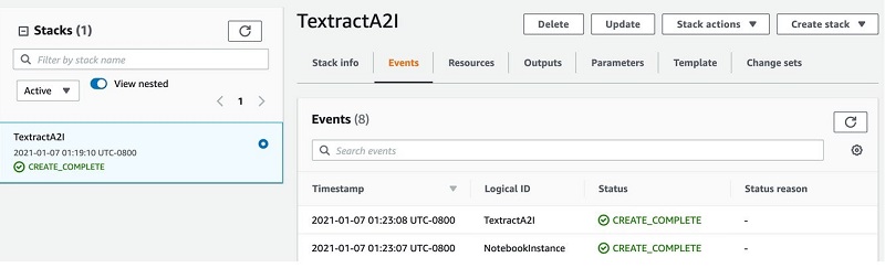
 The following screenshot of the stack details page shows the status of the stack as
 CREATE_IN_PROGRESS. It can take up to 20 minutes for the status to change to CREATE_COMPLETE.
- On the SageMaker console, choose Notebook Instances.
- Choose Open Jupyter for the
TextractA2INotebook notebook you created.
- Open
textract-hand-written-a2i-forms.ipynb and follow along there.
Setting up an Amazon A2I private workforce
For this post, you create a private work team and add only one user (you) to it. For instructions, see Create a Private Workforce (Amazon SageMaker Console). When the user (you) accepts the invitation, you have to add yourself to the workforce. For instructions, see the Add a Worker to a Work Team section in Manage a Workforce (Amazon SageMaker Console).
After you create a labeling workforce, copy the workforce ARN and enter it in the notebook cell to set up a private review workforce:
WORKTEAM_ARN= "<your workteam ARN>"
In the following sections, we walk you through the steps to use this notebook.
Retrieving tabular data from the document and inspecting the response
In this section, we go through the following steps using the walkthrough notebook:
- Review the sample data, which has both printed and handwritten content.
- Set up the helper functions to parse the Amazon Textract response.
- Inspect and analyze the Amazon Textract response.
Reviewing the sample data
Review the sample data by running the following notebook cell:
# Document
documentName = "test_handwritten_document.png"

display(Image(filename=documentName))
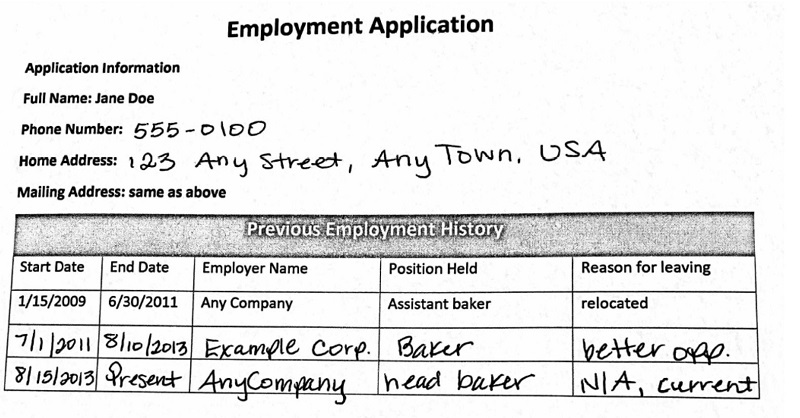
We use the following sample document, which has both printed and handwritten content in tables.
Use the Amazon Textract Parser Library to process the response
We will now import the Amazon Textract Response Parser library to parse and extract what we need from Amazon Textract’s response. There are two main functions here. One, we will extract the form data (key-value pairs) part of the header section of the document. Two, we will parse the table and cells to create a csv file containing the tabular data. In this notebook, we will use Amazon Textract’s Sync API for document extraction, AnalyzeDocument. This accepts image files (png or jpeg) as an input.
client = boto3.client(
         service_name='textract',
         region_name= 'us-east-1',
         endpoint_url='https://textract.us-east-1.amazonaws.com',
)

with open(documentName, 'rb') as file:
        img_test = file.read()
        bytes_test = bytearray(img_test)
        print('Image loaded', documentName)

# process using image bytes
response = client.analyze_document(Document={'Bytes': bytes_test}, FeatureTypes=['TABLES','FORMS'])
You can use the Amazon Textract Response Parser library to easily parse JSON returned by Amazon Textract. The library parses JSON and provides programming language specific constructs to work with different parts of the document. For more details, please refer to the Amazon Textract Parser Library
from trp import Document
# Parse JSON response from Textract
doc = Document(response)

# Iterate over elements in the document
for page in doc.pages:
    # Print lines and words
    for line in page.lines:
        print("Line: {}".format(line.text))
        for word in line.words:
            print("Word: {}".format(word.text))

    # Print tables
    for table in page.tables:
        for r, row in enumerate(table.rows):
            for c, cell in enumerate(row.cells):
                print("Table[{}][{}] = {}".format(r, c, cell.text))

    # Print fields
    for field in page.form.fields:
        print("Field: Key: {}, Value: {}".format(field.key.text, field.value.text))
Now that we have the contents we need from the document image, let’s create a csv file to store it and also use it for setting up the Amazon A2I human loop for review and modification as needed.
# Lets get the form data into a csv file
with open('test_handwritten_form.csv', 'w', newline='') as csvfile:
    formwriter = csv.writer(csvfile, delimiter=',',
                            quoting=csv.QUOTE_MINIMAL)
    for field in page.form.fields:
        formwriter.writerow([field.key.text+" "+field.value.text])

# Lets get the table data into a csv file
with open('test_handwritten_tab.csv', 'w', newline='') as csvfile:
    tabwriter = csv.writer(csvfile, delimiter=',')
    for r, row in enumerate(table.rows):
        csvrow = []
        for c, cell in enumerate(row.cells):
            if cell.text:
                csvrow.append(cell.text.rstrip())
                #csvrow += '{}'.format(cell.text.rstrip())+","
        tabwriter.writerow(csvrow)
Alternatively, if you would like to modify this notebook to use a PDF file or for batch processing of documents, use the StartDocumentAnalysis API. StartDocumentAnalysis returns a job identifier (JobId) that you use to get the results of the operation. When text analysis is finished, Amazon Textract publishes a completion status to the Amazon Simple Notification Service (Amazon SNS) topic that you specify in NotificationChannel. To get the results of the text analysis operation, first check that the status value published to the Amazon SNS topic is SUCCEEDED. If so, call GetDocumentAnalysis, and pass the job identifier (JobId) from the initial call to StartDocumentAnalysis.
Inspecting and analyzing the Amazon Textract response
We now load the form line items into a Pandas DataFrame and clean it up to ensure we have the relevant columns and rows that downstream applications need. We then send it to Amazon A2I for human review.
Run the following notebook cell to inspect and analyze the key-value data from the Amazon Textract response:
# Load the csv file contents into a dataframe, strip out extra spaces, use comma as delimiter
df_form = pd.read_csv('test_handwritten_form.csv', header=None, quoting=csv.QUOTE_MINIMAL, sep=',')
# Rename column
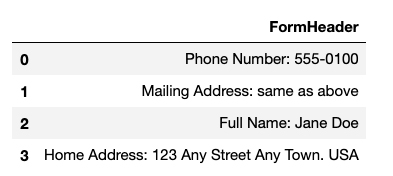
df_form = df_form.rename(columns={df_form.columns[0]: 'FormHeader'})
# display the dataframe
df_form
The following screenshot shows our output.
Run the following notebook cell to inspect and analyze the tabular data from the Amazon Textract response:
# Load the csv file contents into a dataframe, strip out extra spaces, use comma as delimiter
df_tab = pd.read_csv('test_handwritten_tab.csv', header=1, quoting=csv.QUOTE_MINIMAL, sep=',')
# display the dataframe
df_tab.head()
The following screenshot shows our output.
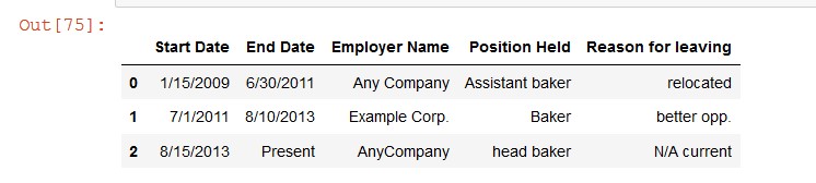
We can see that Amazon Textract detected both printed and handwritten content from the tabular data.
Setting up an Amazon A2I human loop
Amazon A2I supports two built-in task types: Amazon Textract key-value pair extraction and Amazon Rekognition image moderation, and a custom task type that you can use to integrate a human review loop into any ML workflow. You can use a custom task type to integrate Amazon A2I with other AWS services like Amazon Comprehend, Amazon Transcribe, and Amazon Translate, as well as your own custom ML workflows. To learn more, see Use Cases and Examples using Amazon A2I.
In this section, we show how to use the Amazon A2I custom task type to integrate with Amazon Textract tables and key-value pairs through the walkthrough notebook for low-confidence detection scores from Amazon Textract responses. It includes the following steps:
- Create a human task UI.
- Create a workflow definition.
- Send predictions to Amazon A2I human loops.
- Sign in to the worker portal and annotate or verify the Amazon Textract results.
Creating a human task UI
You can create a task UI for your workers by creating a worker task template. A worker task template is an HTML file that you use to display your input data and instructions to help workers complete your task. If you’re creating a human review workflow for a custom task type, you must create a custom worker task template using HTML code. For more information, see Create Custom Worker Task Template.
For this post, we created a custom UI HTML template to render Amazon Textract tables and key-value pairs in the notebook. You can find the template tables-keyvalue-sample.liquid.html in our GitHub repo and customize it for your specific document use case.
This template is used whenever a human loop is required. We have over 70 pre-built UIs available on GitHub. Optionally, you can create this workflow definition on the Amazon A2I console. For instructions, see Create a Human Review Workflow.
After you create this custom template using HTML, you must use this template to generate an Amazon A2I human task UI Amazon Resource Name (ARN). This ARN has the following format: arn:aws:sagemaker:<aws-region>:<aws-account-number>:human-task-ui/<template-name>. This ARN is associated with a worker task template resource that you can use in one or more human review workflows (flow definitions). Generate a human task UI ARN using a worker task template by using the CreateHumanTaskUi API operation by running the following notebook cell:
def create_task_ui():
    '''
    Creates a Human Task UI resource.

    Returns:
    struct: HumanTaskUiArn
    '''
    response = sagemaker_client.create_human_task_ui(
        HumanTaskUiName=taskUIName,
        UiTemplate={'Content': template})
    return response
# Create task UI
humanTaskUiResponse = create_task_ui()
humanTaskUiArn = humanTaskUiResponse['HumanTaskUiArn']
print(humanTaskUiArn)
The preceding code gives you an ARN as output, which we use in setting up flow definitions in the next step:
arn:aws:sagemaker:us-east-1:<aws-account-nr>:human-task-ui/ui-hw-invoice-2021-02-10-16-27-23
Creating the workflow definition
In this section, we create a flow definition. Flow definitions allow us to specify the following:
- The workforce that your tasks are sent to
- The instructions that your workforce receives (worker task template)
- Where your output data is stored
For this post, we use the API in the following code:
create_workflow_definition_response = sagemaker_client.create_flow_definition(
        FlowDefinitionName= flowDefinitionName,
        RoleArn= role,
        HumanLoopConfig= {
            "WorkteamArn": WORKTEAM_ARN,
            "HumanTaskUiArn": humanTaskUiArn,
            "TaskCount": 1,
            "TaskDescription": "Review the table contents and correct values as indicated",
            "TaskTitle": "Employment History Review"
        },
        OutputConfig={
            "S3OutputPath" : OUTPUT_PATH
        }
    )
flowDefinitionArn = create_workflow_definition_response['FlowDefinitionArn'] # let's save this ARN for future use
Optionally, you can create this workflow definition on the Amazon A2I console. For instructions, see Create a Human Review Workflow.
Sending predictions to Amazon A2I human loops
We create an item list from the Pandas DataFrame where we have the Amazon Textract output saved. Run the following notebook cell to create a list of items to be sent for review:
NUM_TO_REVIEW = len(df_tab) # number of line items to review
dfstart = df_tab['Start Date'].to_list()
dfend = df_tab['End Date'].to_list()
dfemp = df_tab['Employer Name'].to_list()
dfpos = df_tab['Position Held'].to_list()
dfres = df_tab['Reason for leaving'].to_list()
item_list = [{'row': "{}".format(x), 'startdate': dfstart[x], 'enddate': dfend[x], 'empname': dfemp[x], 'posheld': dfpos[x], 'resleave': dfres[x]} for x in range(NUM_TO_REVIEW)]
item_list
You get an output of all the rows and columns received from Amazon Textract:
[{'row': '0',
  'startdate': '1/15/2009 ',
  'enddate': '6/30/2011 ',
  'empname': 'Any Company ',
  'posheld': 'Assistant baker ',
  'resleave': 'relocated '},
 {'row': '1',
  'startdate': '7/1/2011 ',
  'enddate': '8/10/2013 ',
  'empname': 'Example Corp. ',
  'posheld': 'Baker ',
  'resleave': 'better opp. '},
 {'row': '2',
  'startdate': '8/15/2013 ',
  'enddate': 'Present ',
  'empname': 'AnyCompany ',
  'posheld': 'head baker ',
  'resleave': 'N/A current '}]
Run the following notebook cell to get a list of key-value pairs:
dforighdr = df_form['FormHeader'].to_list()
hdr_list = [{'hdrrow': "{}".format(x), 'orighdr': dforighdr[x]} for x in range(len(df_form))]
hdr_list
Run the following code to create a JSON response for the Amazon A2I loop by combining the key-value and table list from the preceding cells:
ip_content = {"Header": hdr_list,
              'Pairs': item_list,
              'image1': s3_img_url
             }
Start the human loop by running the following notebook cell:
# Activate human loops
import json
humanLoopName = str(uuid.uuid4())

start_loop_response = a2i.start_human_loop(
            HumanLoopName=humanLoopName,
            FlowDefinitionArn=flowDefinitionArn,
            HumanLoopInput={
                "InputContent": json.dumps(ip_content)
            }
        )
Check the status of human loop with the following code:
completed_human_loops = []
resp = a2i.describe_human_loop(HumanLoopName=humanLoopName)
print(f'HumanLoop Name: {humanLoopName}')
print(f'HumanLoop Status: {resp["HumanLoopStatus"]}')
print(f'HumanLoop Output Destination: {resp["HumanLoopOutput"]}')
print('n')

if resp["HumanLoopStatus"] == "Completed":
    completed_human_loops.append(resp)
You get the following output, which shows the status of the human loop and the output destination S3 bucket:
HumanLoop Name: f69bb14e-3acd-4301-81c0-e272b3c77df0
HumanLoop Status: InProgress
HumanLoop Output Destination: {'OutputS3Uri': 's3://sagemaker-us-east-1-<aws-account-nr>/textract-a2i-handwritten/a2i-results/fd-hw-forms-2021-01-11-16-54-31/2021/01/11/16/58/13/f69bb14e-3acd-4301-81c0-e272b3c77df0/output.json'}
Annotating the results via the worker portal
Run the steps in the notebook to check the status of the human loop. You can use the accompanying SageMaker Jupyter notebook to follow the steps in this post.
- Run the following notebook cell to get a login link to navigate to the private workforce portal:
workteamName = WORKTEAM_ARN[WORKTEAM_ARN.rfind('/') + 1:]
print("Navigate to the private worker portal and do the tasks. Make sure you've invited yourself to your workteam!")
print('https://' + sagemaker_client.describe_workteam(WorkteamName=workteamName)['Workteam']['SubDomain'])
- Choose the login link to the private worker portal.
- Select the human review job.
- Choose Start working.
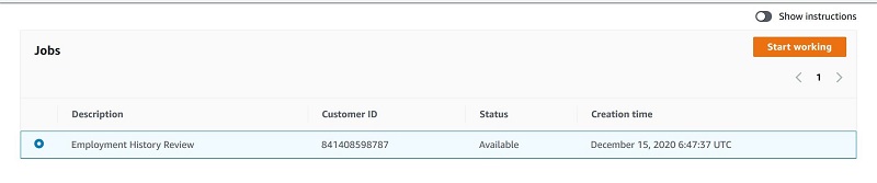
You’re redirected to the Amazon A2I console, where you find the original document displayed, your key-value pair, the text responses detected from Amazon Textract, and your table’s responses.
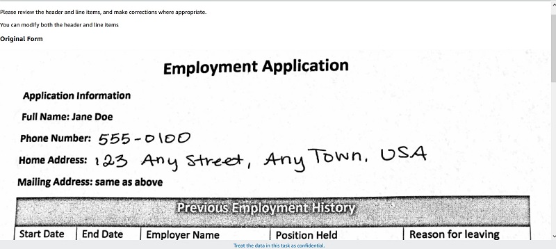
Scroll down to find the correction form for key-value pairs and text, where you can verify the results and compare the Amazon Textract response to the original document. You will also find the UI to modify the tabular handwritten and printed content.
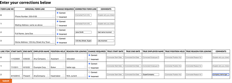
You can modify each cell based on the original image response and reenter correct values and submit your response. The labeling workflow is complete when you submit your responses.
Evaluating the results
When the labeling work is complete, your results should be available in the S3 output path specified in the human review workflow definition. The human answers are returned and saved in the JSON file. Run the notebook cell to get the results from Amazon S3:
import re
import pprint

pp = pprint.PrettyPrinter(indent=4)

for resp in completed_human_loops:
    splitted_string = re.split('s3://' +  'a2i-experiments' + '/', resp['HumanLoopOutput']['OutputS3Uri'])
    output_bucket_key = splitted_string[1]

    response = s3.get_object(Bucket='a2i-experiments', Key=output_bucket_key)
    content = response["Body"].read()
    json_output = json.loads(content)
    pp.pprint(json_output)
    print('n')
The following code shows a snippet of the Amazon A2I annotation output JSON file:
{   'flowDefinitionArn': 'arn:aws:sagemaker:us-east-1:<aws-account-nr>:flow-definition/fd-hw-invoice-2021-02-22-23-07-53',
    'humanAnswers': [   {   'acceptanceTime': '2021-02-22T23:08:38.875Z',
                            'answerContent': {   'TrueHdr3': 'Full Name: Jane '
                                                             'Smith',
                                                 'predicted1': 'relocated',
                                                 'predicted2': 'better opp.',
                                                 'predicted3': 'N/A, current',
                                                 'predictedhdr1': 'Phone '
                                                                  'Number: '
                                                                  '555-0100',
                                                 'predictedhdr2': 'Mailing '
                                                                  'Address: '
                                                                  'same as '
                                                                  'above',
                                                 'predictedhdr3': 'Full Name: '
                                                                  'Jane Doe',
                                                 'predictedhdr4': 'Home '
                                                                  'Address: '
                                                                  '123 Any '
                                                                  'Street, Any '
                                                                  'Town. USA',
                                                 'rating1': {   'agree': True,
                                                                'disagree': False},
                                                 'rating2': {   'agree': True,
                                                                'disagree': False},
                                                 'rating3': {   'agree': False,
                                                                'disagree': True},
                                                 'rating4': {   'agree': True,
                                                                'disagree': False},
                                                 'ratingline1': {   'agree': True,
                                                                    'disagree': False},
                                                 'ratingline2': {   'agree': True,
                                                                    'disagree': False},
                                                 'ratingline3': {   'agree': True,
                                                                    'disagree': False}}
Storing the Amazon A2I annotated results in DynamoDB
We now store the form with the updated contents in a DynamoDB table so downstream applications can use it. To automate the process, simply set up an AWS Lambda trigger with DynamoDB to automatically extract and send information to your API endpoints or applications. For more information, see DynamoDB Streams and AWS Lambda Triggers.
To store your results, complete the following steps:
- Get the human answers for the key-values and text into a DataFrame by running the following notebook cell:
#updated array values to be strings for dataframe assignment
for i in json_output['humanAnswers']:
    x = i['answerContent']

for j in range(0, len(df_form)):
    df_form.at[j, 'TrueHeader'] = str(x.get('TrueHdr'+str(j+1)))
    df_form.at[j, 'Comments'] = str(x.get('Comments'+str(j+1)))


df_form = df_form.where(df_form.notnull(), None)
- Get the human-reviewed answers for tabular data into a DataFrame by running the following cell:
#updated array values to be strings for dataframe assignment
for i in json_output['humanAnswers']:
    x = i['answerContent']

for j in range(0, len(df_tab)):
    df_tab.at[j, 'TrueStartDate'] = str(x.get('TrueStartDate'+str(j+1)))
    df_tab.at[j, 'TrueEndDate'] = str(x.get('TrueEndDate'+str(j+1)))
    df_tab.at[j, 'TrueEmpName'] = str(x.get('TrueEmpName'+str(j+1)))
    df_tab.at[j, 'TruePosHeld'] = str(x.get('TruePosHeld'+str(j+1)))
    df_tab.at[j, 'TrueResLeave'] = str(x.get('TrueResLeave'+str(j+1)))
    df_tab.at[j, 'ChangeComments'] = str(x.get('Change Reason'+str(j+1)))

df_tab = df_tab.where(df_tab.notnull(), None)You will get below output:
- Combine the DataFrames into one DataFrame to save in the DynamoDB table:
# Join both the dataframes to prep for insert into DynamoDB
df_doc = df_form.join(df_tab, how='outer')
df_doc = df_doc.where(df_doc.notnull(), None)
df_doc
Creating the DynamoDB table
Create your DynamoDB table with the following code:
# Get the service resource.
dynamodb = boto3.resource('dynamodb')
tablename = "emp_history-"+str(uuid.uuid4())

# Create the DynamoDB table.
table = dynamodb.create_table(
TableName=tablename,
KeySchema=[
{
'AttributeName': 'line_nr',
'KeyType': 'HASH'
}
],
AttributeDefinitions=[
{
'AttributeName': 'line_nr',
'AttributeType': 'N'
},
],
ProvisionedThroughput={
'ReadCapacityUnits': 5,
'WriteCapacityUnits': 5
}
)
# Wait until the table exists.
table.meta.client.get_waiter('table_exists').wait(TableName=tablename)
# Print out some data about the table.
print("Table successfully created. Item count is: " + str(table.item_count))
You get the following output:
Table successfully created. Item count is: 0
Uploading the contents of the DataFrame to a DynamoDB table
Upload the contents of your DataFrame to your DynamoDB table with the following code:
Note: When adding contents from multiple documents in your DynamoDB table, please ensure you add a document number as an attribute to differentiate between documents. In the example below we just use the index as the line_nr because we are working with a single document.
for idx, row in df_doc.iterrows():
    table.put_item(
       Item={
        'line_nr': idx,
        'orig_hdr': str(row['FormHeader']) ,
        'true_hdr': str(row['TrueHeader']),
        'comments': str(row['Comments']),
        'start_date': str(row['Start Date ']),
        'end_date': str(row['End Date ']),
        'emp_name': str(row['Employer Name ']),
        'position_held': str(row['Position Held ']),
        'reason_for_leaving': str(row['Reason for leaving']),
        'true_start_date': str(row['TrueStartDate']),
        'true_end_date': str(row['TrueEndDate']),
        'true_emp_name': str(row['TrueEmpName']),
        'true_position_held': str(row['TruePosHeld']),
        'true_reason_for_leaving': str(row['TrueResLeave']),
        'change_comments': str(row['ChangeComments'])
        }
    )
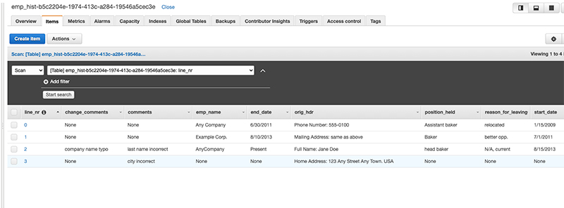
To check if the items were updated, run the following code to retrieve the DynamoDB table value:
response = table.get_item(
Key={
'line_nr': 2
}
)
item = response['Item']
print(item)
Alternatively, you can check the table on the DynamoDB console, as in the following screenshot.
Conclusion
This post demonstrated how easy it is to use services in the AI layer of the AWS AI/ML stack, such as Amazon Textract and Amazon A2I, to read and process tabular data from handwritten forms, and store them in a DynamoDB table for downstream applications to use. You can also send the augmented form data from Amazon A2I to an S3 bucket to be consumed by your AWS analytics applications.
For video presentations, sample Jupyter notebooks, or more information about use cases like document processing, content moderation, sentiment analysis, text translation, and more, see Amazon Augmented AI Resources. If this post helps you or inspires you to solve a problem, we would love to hear about it! The code for this solution is available on the GitHub repo for you to use and extend. Contributions are always welcome!
About the Authors
 Prem Ranga is an Enterprise Solutions Architect based out of Atlanta, GA. He is part of the Machine Learning Technical Field Community and loves working with customers on their ML and AI journey. Prem is passionate about robotics, is an autonomous vehicles researcher, and also built the Alexa-controlled Beer Pours in Houston and other locations.
 Mona Mona is an AI/ML Specialist Solutions Architect based out of Arlington, VA. She works with the World Wide Public Sector team and helps customers adopt machine learning on a large scale. She is passionate about NLP and ML explainability areas in AI/ML.
 Sriharsha M S is an AI/ML specialist solution architect in the Strategic Specialist team at Amazon Web Services. He works with strategic AWS customers who are taking advantage of AI/ML to solve complex business problems. He provides technical guidance and design advice to implement AI/ML applications at scale. His expertise spans application architecture, big data, analytics, and machine learning.
Read More


 Jan Bauer is a Cloud Application Developer at AWS Professional Services. His interests are serverless computing, machine learning, and everything that involves cloud computing.