Integrating Amazon Polly with legacy IVR systems by converting output to WAV format

Amazon Web Services (AWS) offers a rich stack of artificial intelligence (AI) and machine learning (ML) services that help automate several components of the customer service industry. Amazon Polly, an AI generated text-to-speech service, enables you to automate and scale your interactive voice solutions, helping to improve productivity and reduce costs.

You might face common implementation challenges when updating or modifying legacy interactive voice response (IVR) systems that don’t support file formats such as MP3 and PCM. Amazon Polly, in order to minimize response latency, produces synthesis in real-time and streams the results back to the customer in a streamable format (MP3, Ogg/Vorbis or raw PCM samples) while the request is being processed. WAV audio format is not streamable by definition, but a WAV file can be easily created from a PCM stream generated by Polly at the end of synthesis, when all samples are collected and the length of the result can be calculated. This post shows you how to convert Amazon Polly output to a common audio format like WAV.

Converting Amazon Polly file output to WAV

One of the challenges with legacy systems is that they may not support Amazon Polly file outputs like MP3. The output of the Amazon Polly SynthesizeSpeech API call doesn’t support WAV, but some legacy IVRs obtain the audio output in WAV file format, which isn’t supported natively in Amazon Polly. Many of these applications are written in Python and Java.

The following sample code which will help in such situations where audio is in WAV file format not supported natively in Amazon Polly. The sample code converts files from PCM to WAV in Python for inputs given in both SSML and text.

#The following sample code snippet converts files from PCM to WAV in Python for both SSML and non SSML text

#Importing libraries
import boto3
import wave
import os

#Initializing variables
CHANNELS = 1 #Polly's output is a mono audio stream
RATE = 16000 #Polly supports 16000Hz and 8000Hz output for PCM format
OUTPUT_FILE_IN_WAVE = "sample_SSML.wav" #WAV format Output file  name
FRAMES = []
WAV_SAMPLE_WIDTH_BYTES = 2 # Polly's output is a stream of 16-bits (2 bytes) samples

#Initializing Polly Client
polly = boto3.client("polly")

#Input text for conversion
INPUT = "<speak>Hi! I'm Matthew. Hope you are doing well. This is a sample PCM to WAV conversion for SSML. I am a Neural voice and have a conversational style. </speak>" # Input in SSML

WORD = "<speak>"
try:
	if WORD in INPUT: #Checking for SSML input
        #Calling Polly synchronous API with text type as SSML
		response = polly.synthesize_speech(Text=INPUT, TextType="ssml", OutputFormat="pcm",VoiceId="Matthew", SampleRate="16000") #the input to sampleRate is a string value.
	else:
		 #Calling Polly synchronous API with text type as plain text
		response = polly.synthesize_speech(Text=INPUT, TextType="text", OutputFormat="pcm",VoiceId="Matthew", SampleRate="16000")
except (BotoCoreError, ClientError) as error:
    sys.exit(-1)

#Processing the response to audio stream
STREAM = response.get("AudioStream")
FRAMES.append(STREAM.read())

WAVEFORMAT = wave.open(OUTPUT_FILE_IN_WAVE,'wb')
WAVEFORMAT.setnchannels(CHANNELS)
WAVEFORMAT.setsampwidth(WAV_SAMPLE_WIDTH_BYTES)
WAVEFORMAT.setframerate(RATE)
WAVEFORMAT.writeframes(b''.join(FRAMES))
WAVEFORMAT.close()

The following is the sample output from the preceding code:

Conclusion

You can convert Amazon Polly output from PCM to WAV so that you can use Amazon Polly in your legacy IVR, enabling it to support WAV file format output. Try this out for yourself and let us know how it goes in the comments!

You can further refine the converted file using the powerful capabilities available in Amazon Polly like the SynthesizeSpeech request, managing lexicons, reserved characters in SSML, and controlling volume, speaking rate, and pitch.


About the Author

Abhishek Soni is a Partner Solutions Architect at AWS. He works with customers to provide technical guidance for the best outcome of workloads on AWS.

Read More

Introducing Amazon SageMaker Reinforcement Learning Components for open-source Kubeflow pipelines

This blog post was co-authored by AWS and Max Kelsen. Max Kelsen is one of Australia’s leading Artificial Intelligence (AI) and Machine Learning (ML) solutions businesses. The company delivers innovation, directly linked to the generation of business value and competitive advantage to customers in Australia and globally, including Fortune 500 companies. Max Kelsen is also dedicated to reinvesting our expertise and profits to solve the challenges of humankind, focusing on Genomics, AI Safety, and Quantum Computing.

Robots require the integration of technologies such as image recognition, sensing, artificial intelligence, machine learning (ML), and reinforcement learning (RL) in ways that are new to the field of robotics. Today, we’re launching Amazon SageMaker Reinforcement Learning Kubeflow Components supporting AWS RoboMaker, a cloud robotics service, for orchestrating robotics ML workflows. Orchestrating robotics operations to train, simulate, and deploy RL applications is difficult and time-consuming. Now, with SageMaker RL components and pipelines, it’s faster to experiment and manage robotics ML workflows from perception to controls and optimization, and create end-to-end solutions without having to rebuild each time.

Robots are being used more widely in society for purposes that are increasing in sophistication, such as complex assembly, picking and packing, last-mile delivery, environmental monitoring, search and rescue, and assisted surgery. Robotics often involves training complex sequences of behaviors. RL is an emerging ML technique that can help develop solutions for exactly these kinds of problems. It learns complex behaviors without requiring any labeled training data, and can make short-term decisions while optimizing for a long-term goal. For example, when a robot interacts with its environment, this mostly takes place in a simulator. The robot receives a positive or negative reward for actions that it takes. Rewards are computed by a user-defined function that outputs a numeric representation of the actions that should be incentivized. The agent tries to maximize positive rewards, and as a result the model learns an optimal strategy for decision-making.

SageMaker and AWS RoboMaker are two different services streamlined to serve two separate personas: data scientists and roboticists, respectively. SageMaker is a fully managed service that provides every developer and data scientist with the ability to build, train, and deploy ML models quickly. SageMaker RL builds on top of SageMaker, adding pre-packaged RL toolkits and making it easy to integrate any simulation environment. AWS RoboMaker is the most complete cloud solution for robotic developers to simulate, test, and securely deploy robotic applications at scale. Its managed Robot Operating System (ROS) (https://www.ros.org/) and Gazebo (http://gazebosim.org/), an open-source robot simulation software, stacks free up engineering resources and enable you to start building quickly. The task of stitching together machine learning workflows for robotics using Amazon SageMaker and AWS RoboMaker is non-trivial, consuming valuable time for both data scientists and roboticists.

With Amazon SageMaker RL Components for Kubernetes, you can use SageMaker RL Components in your Kubeflow pipelines to invoke and parallelize SageMaker training jobs and AWS RoboMaker simulation jobs as steps in your RL training workflow, without having to worry about how it runs under the hood. The following diagram illustrates the pipeline workflow for SageMaker RL Components

The following diagram illustrates the pipeline workflow for SageMaker RL Components.

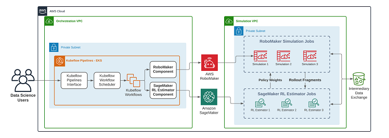
SageMaker Components in your Kubeflow pipeline simply loads the components and describes your pipeline using the Kubeflow Pipelines SDK. SageMaker RL uses open-source libraries such as Anyscale’s Ray to start training an RL agent by collecting experience from Gazebo (an open-source software to simulate populations of robots in complex indoor and outdoor environments) in AWS RoboMaker using ROS (a set of software libraries and tools that help you build robot applications). When the training is completed, the RL agent model is stored in an Amazon Simple Storage Service (Amazon S3) bucket, and an Amazon SageMaker inference node can be created for deployment in production. You can then download the model to the robot with the same ROS structure from the simulation to perform the required tasks.

Although our solution is implemented in Kubeflow components and pipelines, it’s not specific to Kubeflow and can be generalized to MLOps workflows in Argo and Kubernetes to orchestrate parallel robotics ML jobs.

Use case: Woodside Energy deploys robotics in oil and gas environments

Woodside Energy uses AWS RoboMaker with Amazon SageMaker Kubeflow operators to train, tune, and deploy reinforcement learning agents to their robots to perform manipulation tasks that are repetitive or dangerous. This framework will allow the team to iterate and deploy at scale.

“Our team and our partners wanted to start exploring using machine learning methods for robotics manipulation,” says Kyle Saltmarsh, Robotics Engineer at Woodside Energy. “Before we could do this effectively, we needed a framework that would allow us to train, test, tune, and deploy these models efficiently. Utilizing Kubeflow components and pipelines with SageMaker and RoboMaker provides us with this framework and we are excited to have our roboticists and data scientists focus their efforts and time on algorithms and implementation.”

Woodside and AWS engaged Max Kelsen to assist in the development and contribution of the RoboMaker and RLEstimator components that enable the pipelines described in this project. Max Kelsen leverages open source throughout most of its work, and views participation in these communities as strategically important to delivering the best outcomes for our clients.

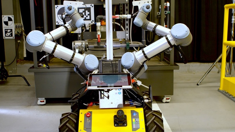
In the following image, Ripley, a custom-built robotics platform by Woodside Energy, is getting ready to perform a double block and bleed, a manual pump shutdown procedure that involves turning multiple valves in sequence. Ripley is based on a Clearpath Robotics Husky equipped with two Universal Robotics UR5 arms, Intel RealSense D435 cameras on each wrist, and a Kodak PixPro body camera. The reinforcement learning formulation utilizes the joint states and camera views as inputs to the agent and outputs optimal trajectories for valve manipulation.

Ripley is a Clearpath Robotics Husky equipped with two Universal Robotics UR5 arms.

Getting started with SageMaker RL components

In a typical Kubeflow pipeline, each component encapsulates your logic in a container image. As a developer or data scientist, you bring in your training, data preprocessing, model serving, or other logic wrapped in a Kubeflow Pipelines ContainerOp function, which builds your code into a new container. Alternatively, you can put the code into a custom container image and push it to a container registry such as Amazon Elastic Container Registry (Amazon ECR). When the pipeline runs, the component’s container is instantiated on one of the worker nodes on the Kubernetes cluster running Kubeflow, and your logic is implemented. Pipeline components can read outputs from the previous components and create outputs that the next component in the pipeline can consume.

When you use SageMaker Components in your Kubeflow pipeline, rather than encapsulating your logic in a custom container, you simply load the components and describe your pipeline using the Kubeflow Pipelines SDK. When the pipeline runs, your instructions are translated into a SageMaker job or deployment. This workload runs on the fully managed infrastructure of SageMaker. You also get all the benefits of a typical SageMaker capability, including Managed Spot Training, automatic scaling of endpoints, and more.

You have separate VPCs for orchestration and simulation. The reason is that no direct communication is needed between the RLEstimator or AWS RoboMaker jobs and the Kubeflow Pipelines components. The components interact directly with the AWS RoboMaker and SageMaker APIs, but not the jobs themselves. The components poll the APIs for the status of the jobs and any related Amazon CloudWatch Logs, and the responses are reflected back to the Kubeflow Pipelines UI. This offers a single interface for viewing the status of the running jobs.

The orchestration VPC utilizes both public and private subnets and a NAT gateway. The Amazon Elastic Kubernetes Service (Amazon EKS) worker nodes are launched into a private network, and use a route to the NAT gateway in the public subnet to interact with AWS APIs, and also to pull public Docker images to run on the cluster. For this post, we allow public access to the EKS cluster endpoint. This allows you to run kubectl port forwarding from your local machine and by doing so open up a tunnel to access the Kubeflow UI. In a production system, we suggest placing the Kubeflow service behind an Application Load Balancer (ALB) and secure using AWS Identity and Access Management (IAM).

Prerequisites

To run the following use case, you need the following:

  • Kubernetes cluster – You can use your existing cluster or create a new one. The fastest way to get one up and running is to launch an EKS cluster using eksctl. For instructions, see Getting started with eksctl. Create a simple cluster with two CPU nodes to run this example. We tested this example on a 2 c5.xlarge. You just need enough node resources to run the SageMaker Component containers and Kubeflow. Training and deployments run on the SageMaker and AWS RoboMaker managed infrastructure.
  • Kubeflow Pipelines – Install Kubeflow Pipelines on your cluster. For instructions, see Step 1 in Deploying Kubeflow Pipelines. Your Kubeflow Pipelines version must be 0.5.0 or above. Optionally, you can install all of Kubeflow, which includes Kubeflow Pipelines.
  • SageMaker and AWS RoboMaker components prerequisites – For instructions on setting up IAM roles and permissions, see Amazon SageMaker Components for Kubeflow Pipelines. You need three IAM roles for the following:
    • Kubeflow pipeline pods to access SageMaker and AWS RoboMaker and launch training and simulation jobs.
    • Amazon SageMaker execution role to access other AWS resources such as Amazon S3.
    • AWS RoboMaker execution role to access other AWS resources such as Amazon S3.

You can launch an EKS cluster from your laptop, desktop, Amazon Elastic Compute Cloud (Amazon EC2) instance, or SageMaker notebook instance. This instance is typically called a gateway instance. Because Amazon EKS offers a fully managed control plane, you only use out-of-the-box the gateway instance to interact with the Kubernetes API and worker nodes. The instance should have a role that allows for interaction with the EKS cluster. The code in the examples here was run from a local device with access to the EKS cluster.

Solution overview

The code, configuration files, and Jupyter notebooks used in this post are available on GitHub. The following walkthrough is provided to explain the key concepts. Rather than copying code from these steps, we recommend running the prepared Jupyter notebook. In this post, we walk through the following high-level steps:

  1. Configure your dependent resources.
  2. Clone the example repository and install dependencies.
  3. Open the example Jupyter notebook.
  4. Install the Kubeflow Pipelines SDK and load SageMaker pipeline components.
  5. Prepare your training datasets and upload them to Amazon S3.
  6. Create your Kubernetes pipeline.
  7. Compile and run your pipeline.

Configuring your dependent resources

If you’re following the proposed architecture from this post, you run the simulation jobs in a private subnet. To ensure that the running jobs have connectivity to AWS resources, add VPC endpoints for the following services:

  • Amazon S3
  • CloudWatch

Next, create an S3 bucket to host your simulation job and RLEstimator job source files. The jobs also use this bucket to communicate by writing config files. The bucket should be in the same Region that you’re running the rest of your infrastructure, because VPC endpoints are locked to accessing resources within the same Region.

Finally, you need to configure an IAM role with access to the S3 bucket and AmazonSageMakerFullAccess and AWSRoboMaker_FullAccess policies.

Cloning the example repository and installing dependencies

Open a terminal and SSH to the EC2 gateway instance that you use to communicate with your EKS cluster. After you log in, clone the example repository to access the example Jupyter notebook. See the following code:

git clone https://github.com/MaxKelsen/kubeflow-pipelines-robomaker-examples
cd kubeflow-pipelines-robomaker-examples
pip install -r requirements.txt

Opening the example Jupyter notebook

As part of the previous step, you installed Jupyter. To open the Jupyter notebook on your gateway instance, complete the following steps:

  1. Launch JupyterLab on your gateway instance and access it on your local machine with the following code:
    jupyter lab

  1. If you’re running the JupyterLab server on an EC2 instance, set up a tunnel to the EC2 instance so you can access the JupyterLab client on your local laptop or desktop. (If you’re using Amazon Linux instead of Ubuntu, you have to use ec2-user as the username. Update the IP address of the EC2 instance and use the appropriate key pair.) See the following code:
    ssh -N -L 0.0.0.0:8081:localhost:8081 -L 0.0.0.0:8888:localhost:8888 -i ~/.ssh/<key_pair>.pem ubuntu@<IP_ADDRESS>

You can now access Jupyter lab at http://localhost:8888 on your local machine.

  1. Access the Kubeflow dashboard by running the following on your gateway instance:
    kubectl port-forward svc/istio-ingressgateway -n istio-system 8081:80

You can now access the Kubeflow dashboard at http://localhost:8081.

Open the example Jupyter notebook (kfp-robomaker-example.ipynb).

SageMaker RLEstimator supports two modes for training jobs (the GitHub repo includes one Jupyter notebook for the latter approach):

  • Bring your own Docker container image – In this mode, you can provide your own Docker container for training. Build your container with your training scripts and push it to Amazon ECR, which is a container registry. SageMaker pulls your container image, instantiates it, and runs training.
  • Bring your own training script (script mode) – In this mode, you don’t have to deal with Docker containers. Simply bring your RLEstimator training scripts in popular frameworks such as TensorFlow, PyTorch, MXNet, and popular RL toolkits such as Coach and Ray, and upload it to Amazon S3. SageMaker automatically pulls the appropriate container, downloads your training scripts, and runs it. This mode is ideal if you don’t want to deal with Docker containers. The kfp-robomaker-example.ipynb Jupyter notebook implements this approach.

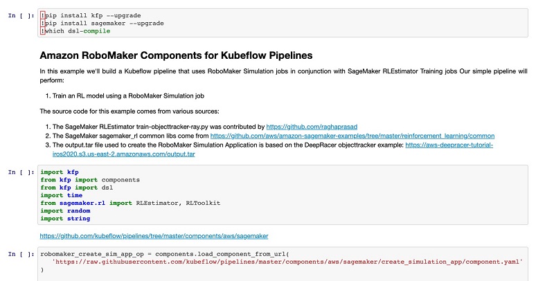
The following example takes a closer look at the first approach (bringing your own Docker container image). You walk through all the important steps in the kfp-robomaker-example.ipynb Jupyter notebook. Having it open makes it easy for you to follow along.

The following screenshot shows the kfp-robomaker-example.ipynb notebook.

The following screenshot shows the kfp-robomaker-example.ipynb notebook.

Installing Kubeflow Pipelines SDK and loading SageMaker pipeline components

To install the SDK and load the pipeline components, complete the following steps:

  1. Install the Kubeflow Pipelines SDK with the following code:
    pip install kfp –upgrade

  1. Import Kubeflow Pipeline packages in Python with the following code:
    import kfp
    from kfp import components
    from kfp.components import func_to_container_op
    from kfp import dsl

  1. Load SageMaker Components in Python with the following code:
    robomaker_create_sim_app_op = components.load_component_from_url('https://raw.githubusercontent.com/kubeflow/pipelines/ 4aa11c3c7f6f068fdb135e1af4a0af5bb1d72d17
    /components/aws/sagemaker/create_simulation_app/component.yaml')
    robomaker_sim_job_op = components.load_component_from_url('https://raw.githubusercontent.com/kubeflow/pipelines/ 4aa11c3c7f6f068fdb135e1af4a0af5bb1d72d17/components/aws/sagemaker/simulation_job/component.yaml')
    robomaker_delete_sim_app_op = components.load_component_from_url( 'https://raw.githubusercontent.com/kubeflow/pipelines/ 4aa11c3c7f6f068fdb135e1af4a0af5bb1d72d17/components/aws/sagemaker/delete_simulation_app/component.yaml')
    sagemaker_rlestimator_op = components.load_component_from_url('https://raw.githubusercontent.com/kubeflow/pipelines/ 4aa11c3c7f6f068fdb135e1af4a0af5bb1d72d17/components/aws/sagemaker/rlestimator/component.yaml')

Preparing training datasets and uploading to Amazon S3

To prepare and upload the source code for SageMaker and AWS RoboMaker, enter the following code:

import boto3
s3 = boto3.resource('s3')
role = "<your_role_name>"
bucket_name = "<your_bucket_name>"
s3.meta.client.upload_file("sourcedir.tar.gz", bucket_name, "sagemaker-sources/sourcedir.tar.gz")
print(f"nUploaded to S3 location: {bucket_name}sagemaker-sources/sourcedir.tar.gz")
s3.meta.client.upload_file("output.tar", bucket_name, "robomaker-sources/output.tar")
print(f"nUploaded to S3 location: {bucket_name}robomaker-sources/output.tar")

Here we upload a sourcedir.tar.gz that contains some object_tracker code that the SageMaker RLEstimator training job uses. We also upload an output.tar file, which contains a colcon bundle that is used to create an AWS RoboMaker simulation application.

Creating a Kubeflow pipeline using AWS RoboMaker and SageMaker Components

You can express a Kubeflow pipeline as a function decorated with @dsl.pipeline, as shown in the following code and in kfp-robomaker-example.ipynb. For more information, see Overview of Kubeflow Pipelines.

@dsl.pipeline(
    name="SageMaker & RoboMaker pipeline",
    description="SageMaker & RoboMaker Reinforcement Learning job where the jobs work together to train an RL model",
)
def sagemaker_robomaker_rl_job(
    region="us-east-1",
    role=role,
    name="robomaker-pipeline-simulation-application"
    + "".join(random.choice(string.ascii_lowercase) for i in range(10)),
    sources=[
        {
            "s3Bucket": bucket_name,
            "s3Key": "robomaker-sources/output.tar",
            "architecture": "X86_64",
        }
    ],
…

In this code example, you create a new function called sagemaker_robomaker_rl_job() and define arguments that are common to all the steps in the pipeline. Within the function, you then define your pipeline components:

  • Creating the simulation application
  • RLEstimator training job
  • AWS RoboMaker simulation jobs
  • Deleting the simulation application

Component 1: Creating the simulation application

This component describes options for creating an AWS RoboMaker simulation application from a colcon bundle file. See the following code:

 robomaker_create_sim_app = robomaker_create_sim_app_op(
        region=region,
        app_name=name,
        sources=sources,
        simulation_software_name=simulation_software_name,
        simulation_software_version=simulation_software_version,
        robot_software_name=robot_software_name,
        robot_software_version=robot_software_version,
        rendering_engine_name=rendering_engine_name,
        rendering_engine_version=rendering_engine_version,
    ).set_display_name('Create RoboMaker Sim App')

The options include the simulation software name and version, the robot software name and version, and also the sources, which are a link to a colcon bundle in Amazon S3.

Component 2: RLEstimator training job

This component describes an SageMaker RLEstimator training job. The job receives data from the AWS RoboMaker simulation jobs and uses that data to train a model. The job issues new policy weights to the simulation jobs while training. See the following code:

rlestimator_training_toolkit_ray = sagemaker_rlestimator_op(
        region=region,
        entry_point=entry_point,
        source_dir=source_dir,
        toolkit=toolkit,
        toolkit_version=toolkit_version,
        framework=framework,
        role=assume_role,
        instance_type=instance_type,
        instance_count=instance_count,
        model_artifact_path=output_path,
        job_name=job_name,
        metric_definitions=metric_definitions,
        max_run=max_run,
        hyperparameters={
            "rl.training.config.lambda": "0.95",
            "robomaker.config.app_arn": robomaker_create_sim_app.outputs["arn"],
            "robomaker.config.num_workers": "3",
            "robomaker.config.packageName": "object_tracker_simulation",
            "robomaker.config.launchFile": "local_client.launch",
            "robomaker.config.policyServerPort": "9000",
            "robomaker.config.iamRole": assume_role,
            "robomaker.config.sagemakerBucket": input_bucket_name,
        },
        vpc_security_group_ids=vpc_security_group_ids,
        vpc_subnets=vpc_subnets,
    ).set_display_name('Start RLEstimator Training')

The options include a reference to the source directory in Amazon S3 where the source code is stored, hyperparameters that are used to configure the training job, and VPC configuration to define where the training job is run. The RLEstimator job spins up a local Redis server that it uses to issue the new policy weights that are consumed by the simulation jobs.

Components 3,4,5: Multiple AWS RoboMaker simulation jobs

These components describe three AWS RoboMaker simulation jobs that use the simulation application created in the robomaker_create_sim_app component. The following code shows one of the components:

robomaker_simulation_job_1 = robomaker_sim_job_op(
        region=region,
        role=role,
        output_bucket=output_bucket,
        output_path=robomaker_output_path,
        max_run=max_run,
        failure_behavior="Fail",
        sim_app_arn=robomaker_create_sim_app.outputs["arn"],
        sim_app_launch_config={
            "packageName": "object_tracker_simulation",
            "launchFile": "local_client.launch",
            "environmentVariables": {
                "RLCAMP_POLICY_SERVER_PORT": "9000",
                "RLCAMP_SAGEMAKER_BUCKET": input_bucket_name,
                "RLCAMP_SAGEMAKER_JOB_NAME": job_name,
                "RLCAMP_AWS_REGION": region,
            },
        },
        vpc_security_group_ids=vpc_security_group_ids,
        vpc_subnets=vpc_subnets,
        use_public_ip="False",
    ).set_display_name('RoboMaker Simulation 1')

Options include the simulation app launch configuration, which includes environment variables that can configure the S3 bucket used for communication between the RLEstimator job and these simulation jobs.

Component 6: Deleting the simulation application

This component is used to delete the simulation application that we created. There is a soft limit of 40 simulation applications per AWS account, so it makes sense to clean up automatically as we create new pipeline runs. See the following code:

robomaker_delete_sim_app = robomaker_delete_sim_app_op(
        region=region, arn=robomaker_create_sim_app.outputs["arn"],
    ).after(
        robomaker_simulation_job_1,
        robomaker_simulation_job_2,
        robomaker_simulation_job_3,
        robomaker_create_sim_app,
    ).set_display_name('Delete RoboMaker Sim App')

The only options are the Region to use to interact with the AWS RoboMaker API and also the ARN of the simulation application to delete. We use the .after() method to define when this component should run as part of the pipeline.

Compiling and running your pipeline

Using the Kubeflow pipeline compiler, you compile the pipeline, create an experiment, and run the pipeline. See the following code:

kfp.compiler.Compiler().compile(sagemaker_robomaker_rl_job,'sagemaker_robomaker_rl_job.zip')
client = kfp.Client()
aws_experiment = client.create_experiment(name='rm-kfp-experiment')
exp_name    = f'sagemaker_robomaker_rl_job-{time.strftime("%Y-%m-%d-%H-%M-%S", time.gmtime())}'
my_run = client.run_pipeline(aws_experiment.id, exp_name, 'sagemaker_robomaker_rl_job.zip')

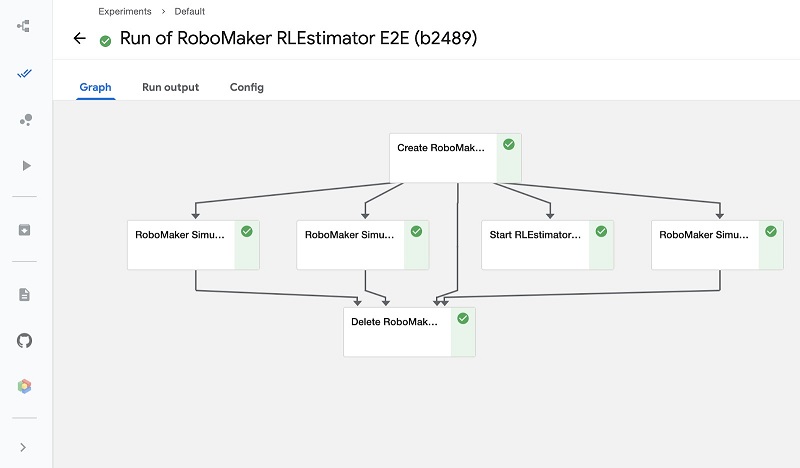
The following is an annotated screenshot of a Kubeflow pipeline after it finishes running. All the steps are SageMaker and AWS RoboMaker capabilities running as part of a Kubeflow pipeline.

The following is an annotated screenshot of a Kubeflow pipeline after it finishes running.

Conclusion

In this post, we discussed using SageMaker RL Components to build open-source Kubeflow pipelines. If you have questions or comments about SageMaker RL Components or AWS RoboMaker components, please leave a comment or create an issue on the Kubeflow Pipelines GitHub repo.


About the Authors

Alex Chung is a Senior Product Manager with AWS in enterprise machine learning systems. His role is to make AWS MLOps products more accessible from Kubernetes and custom environments. He’s passionate about accelerating ML adopted for a large body of users to solve global economic and societal problems. Outside machine learning, he is also a board member at a Silicon Valley nonprofit for donating stock to charityCocatalyst.org.

Kyle Saltmarsh is a robotics engineer from the Intelligent Assets and Robotics group at Woodside Energy. Kyle enjoys rock climbing, long walks on the beach and robot learning.

Leonard O’Sullivan is a Senior Technical Engineer at Max Kelsen, with numerous AWS certifications including SysOps Admin, Developer and Solution Architect. Leonard has more than 8 years of software development experience, and his passion is creating extensible, maintainable and readable code, with a focus on optimizing workflows and removing bottlenecks. Leonard’s current position centres around the automation and optimization of Machine Learning Operations. In his free time, you can find him playing soccer, eating pizza or trying new activities such as axe throwing and hang gliding.

Nicholas Therkelsen-Terry is CEO and Co-Founder of Max Kelsen, a machine learning and artificial intelligence solutions company. Nick has a broad range of expertise spanning across business, economics, sales, management and law. Nick has a deep theoretical and applied understanding of cutting-edge machine learning techniques and has been widely recognized as an expert and thought-leader in this field. Nick is a founding member and board representative of the Queensland AI Hub, a large investment supporting the development of the AI industry, creating more jobs and providing aspiring AI engineers with a space of their own to contribute to Australia’s innovation growth.

Nicholas Thomson is a Software Development Engineer with AWS Deep Learning. He helps build the open-source deep learning infrastructure projects that power Amazon AI. In his free time, he enjoys playing pool or building proof of concept websites.

Ragha Prasad is a software engineer on the AWS RoboMaker team. Primarily interested in robotics and artificial intelligence. In his spare time, he likes to travel, work on art projects and catch up on documentaries.

Sahika Genc is a senior applied scientist at Amazon artificial intelligence (AI). Her research interests are in smart automation, robotics, predictive control and optimization, and reinforcement learning (RL), and she serves in the industrial committee for the International Federation of Automatic Control. She leads science teams in scalable autonomous driving and automation systems, including consumer products such as AWS DeepRacer and SageMaker RL. Previously, she was a senior research scientist in the Artificial Intelligence and Learning Laboratory at the General Electric (GE) Global Research Center.

Read More

Analyzing open-source ML pipeline models in real time using Amazon SageMaker Debugger

Open-source workflow managers are popular because they make it easy to orchestrate machine learning (ML) jobs for productions. Taking models into productions following a GitOps pattern is best managed by a container-friendly workflow manager, also known as MLOps. Kubeflow Pipelines (KFP) is one of the Kubernetes-based workflow managers used today. However, it doesn’t provide all the functionality you need for a best-in-class data science and ML engineer experience. A common issue when developing ML models is having access to the tensor-level metadata of how the job is performing. For extremely large models such as for natural language processing (NLP) and computer vision (CV), this can be critical to avoid wasted GPU resources. However, most training frameworks become a black box after starting to train a model.

Amazon SageMaker is a managed ML platform from AWS to build, train, and deploy ML models at scale. SageMaker Components for Kubeflow Pipelines offer the flexibility to run steps of your KFP workflows on SageMaker instead of on your Kubernetes cluster, which provides the extra capabilities of SageMaker to develop high-quality models. SageMaker Debugger offers the capability to debug ML models during training by identifying and detecting problems with the models in near-real time. This feature can be used when training models within Kubeflow Pipelines through the SageMaker Training component. When combined, you can ensure that if your training jobs aren’t continuously improving with decreasing loss rate, the job ends early, thereby saving both cost and time.

SageMaker Debugger allows you to capture and analyze the state from training with minimal code changes. The state is composed of the following:

  • The parameters being learned by the model, such as weights and biases for neural networks
  • The changes applied to these parameters by the optimizer, called gradients
  • The optimization parameters themselves
  • Scalar values, such as accuracies and losses
  • The output of each layer

The monitoring of these states is done through rules. SageMaker includes a variety of predefined rules, and you can also make custom rules using Python. For more information, see Amazon SageMaker Debugger – Debug Your Machine Learning Models.

In this post, we go over how to deploy a simple pipeline featuring a training component that has a debugger enabled.

Using SageMaker Debugger for Kubeflow Pipelines with XGBoost

This post demonstrates how adding additional parameters to configure the debugger component can allow us to easily find issues within a model. We train a gradient-boosting model on the Modified National Institute of Standards and Technology (MNIST) dataset using Kubeflow Pipelines. The MNIST dataset contains images of handwritten digits from 0–9 and is a popular ML problem. The MNIST dataset contains 60,000 training images and 10,000 test images.

This post walks through the following steps:

  • Generating your data
  • Cloning the sample repository
  • Creating the training pipeline
  • Adding debugger parameters
  • Compiling the pipeline
  • Deploying the training pipeline through Kubeflow Pipelines
  • Reading the debugger output

Prerequisites

To run the example in this post, you need the following prerequisites:

You can run this example from any instance that has Python installed and access to the Kubernetes cluster where Kubeflow pipelines is installed.

Generating your training data

This post uses a SageMaker prebuilt container to train an XGBoost model on the MNIST dataset. We include a Python file that uploads the MNIST dataset to an S3 bucket in the format that the XGBoost prebuilt container expects.

  1. Create an S3 bucket. This post uses the us-east-1 Region.
  2. Create a new file named s3_dsample_data_creator.py with the following code:
    import pickle, gzip, numpy, urllib.request, json
    from urllib.parse import urlparse
    
    ###################################################################
    # This is the only thing that you need to change to run this code 
    # Give the name of your S3 bucket 
    bucket = '<bucket-name>' 
    
    # If you are going to use the default values of the pipeline then 
    # give a bucket name which is in us-east-1 region 
    ###################################################################
    
    
    # Load the dataset
    urllib.request.urlretrieve("http://deeplearning.net/data/mnist/mnist.pkl.gz", "mnist.pkl.gz")
    with gzip.open('mnist.pkl.gz', 'rb') as f:
        train_set, valid_set, test_set = pickle.load(f, encoding='latin1')
    
    
    # Upload dataset to S3
    from sagemaker.amazon.common import write_numpy_to_dense_tensor
    import io
    import boto3
    
    train_data_key = 'mnist_kmeans_example/train_data'
    test_data_key = 'mnist_kmeans_example/test_data'
    train_data_location = 's3://{}/{}'.format(bucket, train_data_key)
    test_data_location = 's3://{}/{}'.format(bucket, test_data_key)
    print('training data will be uploaded to: {}'.format(train_data_location))
    print('training data will be uploaded to: {}'.format(test_data_location))
    
    # Convert the training data into the format required by 
    # the SageMaker XGBoost algorithm
    buf = io.BytesIO()
    write_numpy_to_dense_tensor(buf, train_set[0], train_set[1])
    buf.seek(0)
    
    boto3.resource('s3').Bucket(bucket).Object(train_data_key).upload_fileobj(buf)
    
    # Convert the test data into the format required by XGBoost algorithm
    write_numpy_to_dense_tensor(buf, test_set[0], test_set[1])
    buf.seek(0)
    
    boto3.resource('s3').Bucket(bucket).Object(test_data_key).upload_fileobj(buf)
    
    # Convert the valid data into the format required by XGBoost algorithm
    numpy.savetxt('valid-data.csv', valid_set[0], delimiter=',', fmt='%g')
    s3_client = boto3.client('s3')
    input_key = "{}/valid_data.csv".format("mnist_kmeans_example/input")
    s3_client.upload_file('valid-data.csv', bucket, input_key)
    

  1. Replace <bucket-name> with the name of the bucket you created.

This script requires you to install Python3, boto3, and NumPy.

  1. Run this script by using python3 s3_sample_data_creator.py.
  2. Verify that the data was successfully uploaded.

In your S3 bucket, you should now see a folder called mnist_kmeans_example, and under input, there should be a CSV file named valid-data.

Cloning the sample repository

In a terminal window, clone the Kubeflow pipelines repository and navigate to the directory with the sample code:

git clone https://github.com/kubeflow/pipelines
cd pipelines/samples/contrib/aws-samples/sagemaker_debugger_demo

We now go over how to create the training pipeline debugger-component-demo.py. This folder contains what the final pipeline should be.

Creating a training pipeline

Create a debugger-component-demo.py Python file as our training pipeline. The pipeline specified has poor hyperparameters and results in a poor model. It doesn’t yet have a debugger configured, but can still be compiled and submitted as a training job, and outputs a model.

See the following code:

#!/usr/bin/env python3

import kfp
import json
import os
import copy
from kfp import components
from kfp import dsl


cur_file_dir = os.path.dirname(__file__)
components_dir = os.path.join(cur_file_dir, '../../../../components/aws/sagemaker/')

sagemaker_train_op = components.load_component_from_file(components_dir + '/train/component.yaml')

def training_input(input_name, s3_uri, content_type):
    return {
        "ChannelName": input_name,
        "DataSource": {"S3DataSource": {"S3Uri": s3_uri, "S3DataType": "S3Prefix"}},
        "ContentType": content_type
    }

bad_hyperparameters = {
    'max_depth': '5',
    'eta': '0',
    'gamma': '4',
    'min_child_weight': '6',
    'silent': '0',
    'subsample': '0.7',
    'num_round': '50'
}


@dsl.pipeline(
    name='XGBoost Training Pipeline with bad hyperparameters',
    description='SageMaker training job test with debugger'
)
def training(role_arn="", bucket_name="my-bucket"):
    train_channels = [
        training_input("train", f"s3://{bucket_name}/mnist_kmeans_example/input/valid_data.csv", 'text/csv')
    ]

    training = sagemaker_train_op(
        region='us-east-1',
        # Refer this link for xgboost Registry URLs: https://docs.aws.amazon.com/sagemaker/latest/dg/sagemaker-algo-docker-registry-paths.html
        image='683313688378.dkr.ecr.us-east-1.amazonaws.com/sagemaker-xgboost:0.90-2-cpu-py3',
        hyperparameters=bad_hyperparameters,
        channels=train_channels,
        instance_type='ml.m5.2xlarge',
        model_artifact_path=f's3://{bucket_name}/mnist_kmeans_example/output/model',
        role=role_arn,
    )


if __name__ == '__main__':
    kfp.compiler.Compiler().compile(training, __file__ + '.zip')

Adding debugger parameters

To enable SageMaker Debugger in your training jobs, you need to define the additional parameters to configure the debugger.

First, use debug_hook_config to select the tensor groups you want to collect for analysis and specify the frequency at which you want to save them. debug_hook_config takes in two parameters:

  • S3OutputPath – Points to the Amazon S3 URI where we intend to store our debugging tensors. SageMaker takes care of uploading these tensors transparently during the run.
  • CollectionConfigurations – Enumerates named collections of tensors we want to save. Collections are a convenient way to organize relevant tensors under same umbrella to make it easy to navigate them during analysis. In this particular example, one of the collections we instruct SageMaker Debugger to save is named metrics. We also instruct SageMaker Debugger to save metrics every three iterations.
    # Collections of tensors we want to save
    collections = {
        'feature_importance' : {
            'save_interval': '5'
        },
        'losses' : {
            'save_interval': '10'
        },
        'average_shap': {
            'save_interval': '5'
        },
        'metrics': {
            'save_interval': '3'
        }
    }
    
    
    # Helper method to format CollectionConfigurations
    def format_collection_config(collection_dict):
        output = []
        for key, val in collection_dict.items():
            output.append({'CollectionName': key, 'CollectionParameters': val})
        return output
    
    
    # Helper method to format debug_hook_config
    def training_debug_hook(s3_uri, collection_dict):
        return {
            'S3OutputPath': s3_uri,
            'CollectionConfigurations': format_collection_config(collection_dict)
        }
        
        
    # Provide the debug_hook_config input to the pipeline
    @dsl.pipeline(...)
    def training(role_arn="", bucket_name="my-bucket"):
        ...
        # debug_hook_config containing S3OutputPath and collections to be saved
        training = sagemaker_train_op(
            debug_hook_config=training_debug_hook(f's3://{bucket_name}/mnist_kmeans_example/hook_config', collections),

We also need to specify what rules we want to activate for automatic analysis using debug_rules_config. In this example, we use two SageMaker built-in rules: OverTraining and LossNotDecreasing. As the names suggest, the rules attempt to evaluate if the loss is not decreasing in the tensors captured by the debugging hook during training and also if the model is being over-trained (validation loss should not increase). See the following code:

# Helper method to format debug_rules_config
def training_debug_rules(rule_name, parameters):
    return {
        'RuleConfigurationName': rule_name,
        # Refer this link for Debugger Registry URLs: https://docs.aws.amazon.com/sagemaker/latest/dg/debugger-docker-images-rules.html
        'RuleEvaluatorImage': '503895931360.dkr.ecr.us-east-1.amazonaws.com/sagemaker-debugger-rules:latest',
        'RuleParameters': parameters
    }

# Provide the debug_rule_config input to the pipeline
@dsl.pipeline(...)
def training(role_arn="", bucket_name="my-bucket"):
    ...
    # Rules and rule parameters
    train_debug_rules = [
        training_debug_rules("LossNotDecreasing", {"rule_to_invoke": "LossNotDecreasing", "tensor_regex": ".*"}),
        training_debug_rules("Overtraining", {'rule_to_invoke': 'Overtraining', 'patience_train': '10', 'patience_validation': '20'}),
    ]
    training = sagemaker_train_op(
        # Provide the debug_rule_config as input to the pipeline
        debug_rule_config=train_debug_rules,
        ...
    )

For more information about SageMaker rules and the configurations best suited for using them, see Amazon SageMaker Debugger RulesConfig.

The following code shows what the pipeline looks like after configuring the debug hook and rules:

#!/usr/bin/env python3

import kfp
import json
import os
import copy
from kfp import components
from kfp import dsl


cur_file_dir = os.path.dirname(__file__)
components_dir = os.path.join(cur_file_dir, '../../../../components/aws/sagemaker/')

sagemaker_train_op = components.load_component_from_file(components_dir + '/train/component.yaml')

def training_input(input_name, s3_uri, content_type):
    return {
        "ChannelName": input_name,
        "DataSource": {"S3DataSource": {"S3Uri": s3_uri, "S3DataType": "S3Prefix"}},
        "ContentType": content_type
    }


def training_debug_hook(s3_uri, collection_dict):
    return {
        'S3OutputPath': s3_uri,
        'CollectionConfigurations': format_collection_config(collection_dict)
    }


def training_debug_rules(rule_name, parameters):
    return {
        'RuleConfigurationName': rule_name,
        # Refer this link for Debugger Registry URLs: https://docs.aws.amazon.com/sagemaker/latest/dg/debugger-docker-images-rules.html
        'RuleEvaluatorImage': '503895931360.dkr.ecr.us-east-1.amazonaws.com/sagemaker-debugger-rules:latest',
        'RuleParameters': parameters
    }


def format_collection_config(collection_dict):
    output = []
    for key, val in collection_dict.items():
        output.append({'CollectionName': key, 'CollectionParameters': val})
    return output


collections = {
    'feature_importance' : {
        'save_interval': '5'
    },
    'losses' : {
        'save_interval': '10'
    },
    'average_shap': {
        'save_interval': '5'
    },
    'metrics': {
        'save_interval': '3'
    }
}


bad_hyperparameters = {
    'max_depth': '5',
    'eta': '0',
    'gamma': '4',
    'min_child_weight': '6',
    'silent': '0',
    'subsample': '0.7',
    'num_round': '50'
}


@dsl.pipeline(
    name='XGBoost Training Pipeline with bad hyperparameters',
    description='SageMaker training job test with debugger'
)
def training(role_arn="", bucket_name="my-bucket"):
    train_channels = [
        training_input("train", f"s3://{bucket_name}/mnist_kmeans_example/input/valid_data.csv", 'text/csv')
    ]
    train_debug_rules = [
        training_debug_rules("LossNotDecreasing", {"rule_to_invoke": "LossNotDecreasing", "tensor_regex": ".*"}),
        training_debug_rules("Overtraining", {'rule_to_invoke': 'Overtraining', 'patience_train': '10', 'patience_validation': '20'}),
    ]
    training = sagemaker_train_op(
        region='us-east-1',
        # Refer this link for xgboost Registry URLs: https://docs.aws.amazon.com/sagemaker/latest/dg/sagemaker-algo-docker-registry-paths.html
        image='683313688378.dkr.ecr.us-east-1.amazonaws.com/sagemaker-xgboost:0.90-2-cpu-py3',
        hyperparameters=bad_hyperparameters,
        channels=train_channels,
        instance_type='ml.m5.2xlarge',
        model_artifact_path=f's3://{bucket_name}/mnist_kmeans_example/output/model',
        debug_hook_config=training_debug_hook(f's3://{bucket_name}/mnist_kmeans_example/hook_config', collections),
        debug_rule_config=train_debug_rules,
        role=role_arn,
    )


if __name__ == '__main__':
    kfp.compiler.Compiler().compile(training, __file__ + '.zip')

Compiling the pipeline

Our pipeline is now complete and ready to be compiled using the following command:

dsl-compile --py debugger-component-demo.py --output debugger-component-demo.tar.gz

This creates debugger-component-demo.tar.gz in the same folder, and is the file we upload as our training job.

Deploying the pipeline

Now use kubectl to open up the KFP UI on our browser so we have access to the interface where we can upload the pipeline.

  1. In a new terminal window, run the following command (it’s possible to create pipelines and submit training jobs from the AWS Command Line Interface (AWS CLI)):
    $ kubectl port-forward -n kubeflow service/ml-pipeline-ui 8080:80

  1. Access the KFP UI by searching http://localhost:8080/ in your browser.
  2. Create a new pipeline and upload the compiled specification (.tar.gz file) as a new pipeline template.
  3. Provide the role_arn and bucket_name you created as pipeline inputs.

Reading the debugger output

When the training is complete, the logs display the status of each debugger rule.

The following screenshot shows an example of what the status of each debugger rule should be when the training job is complete.

The following screenshot shows an example of what the status of each debugger rule should be when the training job is complete.

We see here that our debugger rules haven’t found any issues with the model being overtrained. However, the debug rules indicate that our loss isn’t decreasing over time as it should.

The following screenshot shows the Amazon CloudWatch Logs, also printed on the Logs tab, which indeed show that the train-rmse is staying steady at 0.5 and isn’t decreasing.

The following screenshot shows the Amazon CloudWatch logs, also printed on the Logs tab, which indeed show that the train-rmse is staying steady at 0.5 and isn’t decreasing.

The reason that our loss isn’t decreasing is because our hyperparameters have been initialized suboptimally, specifically eta, which has been set to a poor value. eta determines the model’s learning rate and is currently at 0. This is clearly erroneous because it means that the subsequent steps aren’t progressing from the initial step. To address, this, use a non-zero learning rate, for example, set eta in hyperparameters to 0.2. You can see that the LossNotDecreasing rule is not triggered as train-rmse keeps decreasing steadily throughout the entire training duration. Rerunning the pipeline with the fix results in a model with no issues found.

Conclusion

Model debugging tools are critical to reduce total time, cost, and resources spent on creating a model. Using SageMaker Debugger in your Kubeflow Pipelines lets you go beyond just looking at scalars like losses and accuracies during training. You can get full visibility into all tensors flowing through the graph during training. Furthermore, it helps you monitor your training in near-real time using rules, and provides alerts if it detects an inconsistency in the training flow, which ultimately reduces costs and improves your company’s effectiveness on ML.

To get started using Kubeflow Pipelines with SageMaker, see the GitHub repo. You can also explore our native integration of SageMaker Operators for Kubernetes for MLOps.


About the Authors

Alex Chung is a Senior Product Manager with AWS in Deep Learning. His role is to make AWS Deep Learning products more accessible and cater to a wider audience. He’s passionate about social impact and technology, getting his regular gym workout, and cooking healthy meals.


Suraj Kota is a Software Engineer specialized in Machine Learning infrastructure. He builds tools to easily get started and scale machine learning workload on AWS. He worked on the Amazon Deep Learning Containers, Deep Learning AMI, SageMaker Operators for Kubernetes, and other open source integrations like Kubeflow.


Dustin Luong is a Software Development Engineering Intern with AWS in Deep Engines. He works on developing SageMaker integrations with open source platforms like Kubernetes and Kubeflow Pipelines. He’s currently a student at UC Berkeley and in his spare time he enjoys playing basketball, hiking, and playing board games.

Read More

Transfer Learning for Audio Data with YAMNet

Posted by Luiz GUStavo Martins, Developer Advocate

Transfer learning is a popular machine learning technique, in which you train a new model by reusing information learned by a previous model. Most common applications of transfer learning are for the vision domain, to train accurate image classifiers, or object detectors, using a small amount of data — or for text, where pre-trained text embeddings or language models like BERT are used to improve on natural language understanding tasks like sentiment analysis or question answering. In this article, you’ll learn how to use transfer learning for a new and important type of data: audio, to build a sound classifier.

There are many important use cases of audio classification, including to protect wildlife, to detect whales and even to fight against illegal deforestation.

With YAMNet, you can create a customized audio classifier in a few easy steps:

  • Prepare and use a public audio dataset
  • Extract the embeddings from the audio files using YAMNet
  • Create a simple two layer classifier and train it.
  • Save and test the final model

You can follow the code here in this tutorial.

The YAMNet model

YAMNet (“Yet another Audio Mobilenet Network”) is a pretrained model that predicts 521 audio events based on the AudioSet corpus.

This model is available on TensorFlow Hub including the TFLite and TF.js versions, for running the model on mobile and the web. The code can be found on their repository.

The model has 3 outputs:

  • Class scores that you’d use for inference
  • Embeddings, which are the important part for transfer learning
  • Log Mel Spectrograms to provide a visualization of the input signal

The model takes a waveform represented as 16 kHz samples in the range [-1.0, 1.0], frames it in windows of 0.96 seconds and hop of 0.48 seconds, and then runs the core of the model to extract the embeddings on a batch of these frames.

The 0.96 seconds windows hopping over a waveform

As an example, trying the model with this audio file [link] will give you these results:

The first graph is the waveform. The second graph is the log-mel spectrogram. The third graph shows the class probability predictions per frame of audio, where darker is more likely.

The ESC-50 dataset

To do transfer learning with the model, you’ll use the Dataset for Environmental Sound Classification, or ESC-50 for short. This is a collection of 2000 environmental audio recordings from 50 classes. Each recording is 5 seconds long and they came originally from the Freesound project.

The ESC-50 has the classes Dog and Cat that you’ll need.

The dataset has two important components: the audio files and a metadata csv file with the metadata about every audio file.

The columns in the metadata csv file contains information that will be used to train the model:

  • Filename gives the name of the .wav audio file
  • Category is the human-readable class name for the numeric target id
  • Target is the unique numeric id of the category
  • Fold ensures that clips originating from the same initial source are always contained in the same group. This is important to avoid cross-contamination when splitting the data into train, validation and test sets and for cross-validation.

For more detailed information you can read the original ESC paper.

Working with the dataset

To load the dataset, you’ll start from the metadata file and load it using the Pandas method read_csv.

With the loaded dataframe, the next steps are to filter by the classes that will be used, in this case: Dogs and Cats.

Next step would be to load the audio files to start the process but if there are too many audio files, just loading all of them to memory can be prohibitive and lead to out of memory issues. The best solution is to lazily load the audio files when needed. TensorFlow can help do this easily with tf.data.Dataset and the map method.

Let’s create the Dataset from the the previous created pandas dataframe and apply the load_wav method to all the files:

filenames = filtered_pd['filename']
targets = filtered_pd['target']
folds = filtered_pd['fold']

main_ds = tf.data.Dataset.from_tensor_slices((filenames, targets, folds))
main_ds = main_ds.map(load_wav_for_map)

Here, no audio file was loaded to memory yet since the mapping wasn’t evaluated. For example, if you request a size of the dataset for example (len(list(train_ds.as_numpy_iterator()))

), that would make the map function to be evaluated and load all the files.

The same technique will be used to extract all the features (embeddings) from each audio file.

Extracting the audio embeddings

Here you are going to load the YAMNet model from TensorFlow Hub. All you need is the model’s handle, and call the load method from the tensorflow_hub library.

yamnet_model_handle = 'https://tfhub.dev/google/yamnet/1'
yamnet_model = hub.load(yamnet_model_handle)

This will load the model to memory ready to be used.

For each audio file, you’ll extract the embeddings using the YAMNet model. For each audio file, YAMNet is executed. The embeddings output is paired with the same label and folder from the audio file.

def extract_embedding(wav_data, label, fold):
''' run YAMNet to extract embedding from the wav data '''
scores, embeddings, spectrogram = yamnet_model(wav_data)
num_embeddings = tf.shape(embeddings)[0]
return (embeddings,
tf.repeat(label, num_embeddings),
tf.repeat(fold, num_embeddings))

main_ds = main_ds.map(extract_embedding).unbatch()

These embeddings will be the input for the classification model. From the model’s documentation, you can read that for a given audio file, it will frame the waveform into sliding windows of length 0.96 seconds and hop 0.48 seconds, and then run the core of the model. So, in summary, for each 0.48 seconds, the model will output one embedding array with 1024 float values. This part is also done using map(), so again, lazy evaluation and that’s why it executes so fast.

The final dataset contains the three used columns: embedding, label and fold.

The last dataset operation is to split into train, validation and test datasets. To do so the filter() method and use the fold field (an integer between 1 and 5) as criteria.

cached_ds = main_ds.cache()
train_ds = cached_ds.filter(lambda embedding, label, fold: fold < 4)
val_ds = cached_ds.filter(lambda embedding, label, fold: fold == 4)
test_ds = cached_ds.filter(lambda embedding, label, fold: fold == 5)

Training the Classifier

With the YAMNet embedding vectors and the label, the next step is to train a classifier that learns what’s a dog’s sound and what is a cat’s sound.

The classifier model is very simple with just two dense layers, but as you’ll see this is enough for the amount of data used.

my_model = tf.keras.Sequential([
tf.keras.layers.Input(shape=(1024), dtype=tf.float32, name='input_embedding'),
tf.keras.layers.Dense(512, activation='relu'),
tf.keras.layers.Dense(len(my_classes))
])

Saving the final model

The model that was trained works and has good accuracy but the input it expects is not an audio waveform but an embedding array. To address this problem, the final model will combine YAMNet as the input layer and the model just trained. This way, the final model will accept a waveform and output the class:

input_segment = tf.keras.layers.Input(shape=(), dtype=tf.float32,
name='audio')
embedding_extraction_layer = hub.KerasLayer('https://tfhub.dev/google/yamnet/1', trainable=False)
scores, embeddings, spectrogram = embedding_extraction_layer(input_segment)
serving_outputs = my_model(embeddings_output)
serving_outputs = ReduceMeanLayer(axis=0, name='classifier')(serving_outputs)
serving_model = tf.keras.Model(input_segment, serving_outputs)
serving_model.save(saved_model_path, include_optimizer=False)

To try the reloaded model, you can use the same way it was used earlier in the colab:

reloaded_model = tf.saved_model.load(saved_model_path)
reloaded_results = reloaded_model(testing_wav_data)
cat_or_dog = my_classes[tf.argmax(reloaded_results)]

This model can also be used with TensorFlow Serving with the ‘serving_default’

serving_results =  reloaded_model.signatures['serving_default'](testing_wav_data)
cat_or_dog = my_classes[tf.argmax(serving_results['classifier'])]

In this post, you learned how to use the YAMNet model for transfer learning to recognize audio of dogs and cats from the ESC-50 dataset.

Check out the YAMNet model on tfhub.dev and the tutorial on tensorflow.org. You can apply this technique to your own dataset, or to other classes in the ESC-50 dataset.

We would love to know what you can build with this! Share your project with us on social media by using the hashtag #TFHub.

Acknowledgements

We’d like to thank a number of colleagues for their contribution to this work: Dan Ellis, Manoj Plakal and Eduardo Fonseca for an amazing YAMNet model and support with the colab and multiple reviews.

Mark Daoust and Elizabeth Kemp have greatly improved the presentation of the material in this post and the associated tutorial.

Read More

NVIDIA’s Marc Hamilton on Building Cambridge-1 Supercomputer During Pandemic

Since NVIDIA announced construction of the U.K.’s most powerful AI supercomputer — Cambridge-1 — Marc Hamilton, vice president of solutions architecture and engineering, has been (remotely) overseeing its building across the pond.

The system, which will be available for U.K. healthcare researchers to work on pressing problems, is being built on NVIDIA DGX SuperPOD architecture for a whopping 400 petaflops of AI performance.

Located at Kao Data, a data center using 100 percent renewable energy, Cambridge-1 would rank among the world’s top three most energy-efficient supercomputers on the latest Green500 list.

Hamilton points to the concentration of leading healthcare companies in the U.K. as a primary reason for NVIDIA’s decision to build Cambridge-1.

AstraZeneca, GSK, Guy’s and St Thomas’ NHS Foundation Trust, King’s College London, and Oxford Nanopore have already announced their intent to harness the supercomputer for research in the coming months.

Construction has been progressing at NVIDIA’s usual speed-of-light pace, with just final installations and initial tests remaining.

Hamilton promises to provide the latest updates on Cambridge-1 at GTC 2021.

Key Points From This Episode:

  • Hamilton gives listeners an explainer on Cambridge-1’s scalable units, or building blocks — NVIDIA DGX A100 systems — and how just 20 of them can provide the equivalent of hundreds of CPUs.
  • NVIDIA intends for Cambridge-1 to accelerate corporate research in addition to that of universities. Among them are King’s College London, which has already announced that it’ll be using the system.

Tweetables:

“With only 20 [DGX A100] servers, you can build one of the top 500 supercomputers in the world” — Marc Hamilton [9:14]

“This is the first time we’re taking an NVIDIA supercomputer by our engineers and opening it up to our partners, to our customers, to use” — Marc Hamilton [10:17]

You Might Also Like:

How AI Can Improve the Diagnosis and Treatment of Diseases

Medicine — particularly radiology and pathology — have become more data-driven. The Massachusetts General Hospital Center for Clinical Data Science — led by Mark Michalski — promises to accelerate that, using AI technologies to spot patterns that can improve the detection, diagnosis and treatment of diseases.

NVIDIA Chief Scientist Bill Dally on Where AI Goes Next

This podcast is full of words from the wise. One of the pillars of the computer science world, NVIDIA’s Bill Dally joins to share his perspective on the world of deep learning and AI in general.

The Buck Starts Here: NVIDIA’s Ian Buck on What’s Next for AI

Ian Buck, general manager of accelerated computing at NVIDIA, shares his insights on how relatively unsophisticated users can harness AI through the right software. Buck helped lay the foundation for GPU computing as a Stanford doctoral candidate, and delivered the keynote address at GTC DC 2019.

The post NVIDIA’s Marc Hamilton on Building Cambridge-1 Supercomputer During Pandemic appeared first on The Official NVIDIA Blog.

Read More