Automate annotation of image training data with Amazon Rekognition

Every machine learning (ML) model demands data to train it. If your model isn’t predicting Titanic survival or iris species, then acquiring a dataset might be one of the most time-consuming parts of your model-building process—second only to data cleaning.

What data cleaning looks like varies from dataset to dataset. For example, the following is a set of images tagged robin that you might want to use to train an image recognition model on bird species.

That nest might count as dirty data, and some model applications may make it inappropriate to include American and European robins in the same category, but this seems pretty good so far. Let’s keep looking at additional images.

Well, that’s clearly not right.

One thing that can be frustrating about bad data is its obvious wrongness—that roaring campfire and woman with a bow and arrow (perhaps doing a Robin Hood-themed photoshoot?) aren’t even birds, much less robins. If your image collections or datasets weren’t carefully assembled by human intelligence for the specific model training application, they’re likely dirty. Cleaning that kind of dirty data is where Amazon Rekognition comes in.

Solution overview

Amazon Rekognition Image is an image recognition service capable of detecting thousands of different objects using deep neural network models. By taking advantage of the training that’s already gone into the service, you can easily sort through a mass of data and pick out only images that contain a known object, whether that’s as general as animal or as specific as robin. This can lead to the development of a customized dataset narrowly suited for your needs that’s cleaned quickly and cheaply compared to manual solutions. You can apply this principle to any image repository that is expected to include a mix of correct and incorrect images, as long as the correct images fall under an existing Amazon Rekognition label that excludes some incorrect images.

Consider one alternative, Amazon Mechanical Turk, a crowdsourcing marketplace where people can post jobs for virtual gig workers. The minimum price of a task (in this case, one worker labeling an image as “a robin” or “not a robin”) is $0.012. To ensure quality, typical jobs on Mechanical Turk have three to five people view and label each image, bringing the cost floor up to $0.036–$0.06 per image. On Amazon Rekognition, the first million images (beyond the Free Tier, which covers 5,000 images a month for 12 months) each cost $0.001, or at most one twelfth the cost of using Mechanical Turk. For distinctions that don’t require human discernment, that can add up to considerable cost savings.

On top of that, you may desire to control costs by limiting the number of images scanned by Amazon Rekognition. We have a couple options for large repositories that might incur substantial costs if searched exhaustively:

  • Place a cap on the number of images to scan. If you want to end up with 50 filtered images for a particular label, like bird, you might set your algorithm to scan only up to several hundred at most. You might end up with fewer than 50 birds—but if the hit rate was so low that you reached the cap, your repository might not be a great source of bird pictures, and you’ve saved money searching to the end for the fiftieth bird. Ideally, you’ll find 50 birds before reaching the cap and stop then, but it’s the nature of dirty data that we often don’t know exactly how dirty it is.
  • Implement an early stopping algorithm. If some number, perhaps 20, images in a row fail to turn up any birds, then stop looking. Early stopping might mean the dataset is unsuited to its intended purpose, or that there was some error in the invocation of the function, like a typo in the label (for example a search for birb instead of bird).

Try the demo filter function

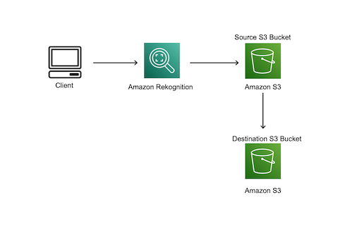
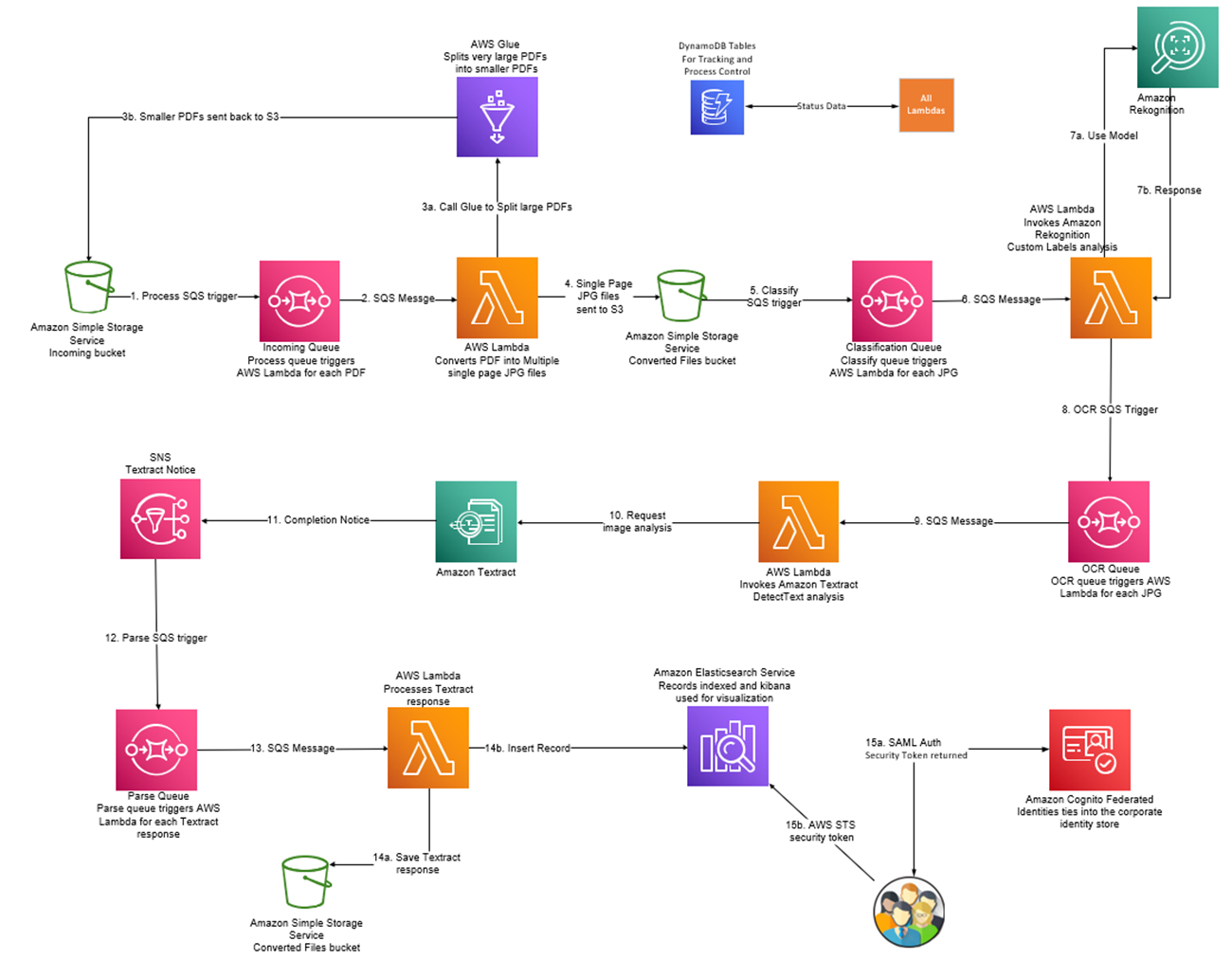
The following diagram shows what this solution could look like in practice. A filter function running locally on the client’s computer can use an SDK to make API calls to Amazon Rekognition and Amazon Simple Storage Service (Amazon S3) to check each image in turn. When Amazon Rekognition detects the desired label in an image from the source bucket repository, the function copies that image into the destination bucket.

All the function needs are appropriate permissions within your AWS account and the following parameters:

  • An Amazon Rekognition label to filter on. To find out which one might be best for your needs, check the current list of available labels (available in the documentation) or try testing a good image from your repository on the Amazon Rekognition console and seeing what labels come up.
  • The name of a source bucket in Amazon S3 that contains an unsorted image repository.
  • The name of a destination bucket that images are copied into if Amazon Rekognition detects the specified label.

Optionally, you can also specify a confidence threshold to even more stringently filter images, and a name to call the folder that images in the destination bucket are organized into.

A basic filter function might look something like this:

def check_for_tag(client, file_name, bucket, tag, threshold):
    """Checks an individual S3 object for a single tag"""

    response = client.detect_labels(
        Image={
            'S3Object': {
                'Bucket': bucket,
                'Name': file_name
            }
        })

    return tag.lower() in {label['Name'].lower() for label in response['Labels'] if label['Confidence'] > threshold}
def filter(source, destination, tag, threshold, name):
    """Copies an object from source to destination if there's a tag match"""

    # set up resources
    s3_resource = boto3.resource('s3')
    client = boto3.client('rekognition')

    # iterate through source bucket, copying hits
    source_bucket = s3_resource.Bucket(source)
    objects = source_bucket.objects.all()
    for object in objects:
        if check_for_tag(client, object.key, source, tag, threshold):
            copy_source = {
                'Bucket': source,
                'Key': object.key
            }
            new_name = f"{name}/{object.key}"
            s3_resource.meta.client.copy(copy_source, destination, new_name)

With the images already stored in Amazon S3, you don’t even need to upload them to Amazon Rekognition to get a prompt response.

The following are some ideas for customizing and exploring this procedure:

  • Add a human-in-the-loop element to the filter function, so that for Amazon Rekognition confidence scores between certain values, the image is sent elsewhere for manual checking.
  • Include the bounding box data from Amazon Rekognition as metadata to train an object detection model.
  • Train an Amazon Rekognition Custom Labels model with the collected data—the filter function above stores images in the format expected by Amazon Rekognition Custom Labels, with each folder’s name corresponding to a label the model predicts.

Conclusion

In this post, we explored the possibility of using Amazon Rekognition to filter image sets intended for ML applications. This solution can remove egregiously off-the-mark images from a dataset, which results in cleaner training data and better-performing models at a fraction of the cost of hiring human data labelers.

Interested in learning about ML through blogs, tutorials, and more? Check out the AWS Machine Learning community.


About the Authors

Samantha Finley is an Associate Solutions Architect at AWS.


Quentin Morris is an Associate Solutions Architect at AWS.


Jerry Mullis is an Associate Solutions Architect at AWS.


Woodrow Bogucki is an Associate Technical Trainer at AWS. He has a Master’s Degree in Computer Engineering from Texas A&M. His favorite class was Deep Learning and his personal interests include Mexican food, BBQ, and fried chicken.

Read More

Simplify patient care with a custom voice assistant using Amazon Lex V2

For the past few decades, physician burnout has been a challenge in the healthcare industry. Although patient interaction and diagnosis are critical aspects of a physician’s job, administrative tasks are equally taxing and time-consuming. Physicians and clinicians must keep a detailed medical record for each patient. That record is stored in the hospital electronic health record (EHR) system, a database that contains the records of every patient in the hospital. To maintain these records, physicians often spend multiple hours each day to manually enter data into the EHR system, resulting in lower productivity and increased burnout.

Physician burnout is one of the leading factors that lead to depression, fatigue, and stress for doctors during their careers. In addition, it can lead to higher turnover, reduced productivity, and costly medical errors, affecting people’s lives and health.

In this post, you learn the importance of voice assistants and how they can automate administrative tasks for doctors. We also walk through creating a custom voice assistant using PocketSphinx and Amazon Lex.

Voice assistants as a solution to physician burnout

Voice assistants are now starting to automate the vital yet manual parts of patient care. They can be a powerful tool to help doctors save time, reduce stress, and spend more time focusing on the patient versus the administrative requirements of clinical documentation.

Today, voice assistants are becoming more available as natural language processing models advance, errors decrease, and development becomes more accessible for the average developer. However, most devices are limited, so developers must often build their own customized versions.

As Solutions Architects working in the healthcare industry, we see a growing trend towards the adoption of voice assistants in hospitals and patient rooms.

In this post, you learn how to create a custom voice assistant using PocketSphinx and Amazon Lex. With our easy-to-set-up and managed services, developers and innovators can hit the ground running and start developing the devices of the future.

Custom voice assistant solution architecture

The following architecture diagram presents the high-level overview of our solution.

In our solution, we first interface with a voice assistant script that runs on your computer. After the wake word is recognized, the voice assistant starts recording what you say and sends the audio to Amazon Lex, where it uses an AWS Lambda function to retrieve dummy patient data stored in Amazon DynamoDB. The sensor data is generated by another Python script, generate_data.py, which you also run on your computer.

Sensor types include blood pressure, blood glucose, body temperature, respiratory rate, and heart rate. Amazon Lex sends back a voice message, and we use Amazon Polly, a service that turns text into lifelike speech, to create a consistent experience.

Now you’re ready to create the components needed for this solution.

Deploy your solution resources

You can find all the files of our custom voice assistant solution on our GitHub repo. Download all the files, including the PocketSphinx model files downloaded from their repo.

You must deploy the DynamoDB table and Lambda function directly by choosing Launch Stack.

The AWS CloudFormation stack takes a few minutes to complete. When it’s complete, you can go to the Resources tab to check out the Lambda function and DynamoDB table created. Note the name of the Lambda function because we reference it later when creating the Amazon Lex bot.

Create the Amazon Lex bot

When the CloudFormation stack is complete, we’re ready to create the Amazon Lex bot. For this post, we use the newer V2 console.

  1. On the Amazon Lex console, choose Switch to the new Lex V2 console.
  2. In the navigation pane, choose Bots.
  3. Choose Create bot.
  4. For Bot name, enter Healthbot.
  5. For Description, enter an optional description.
  6. For Runtime role, select Create a role with basic Amazon Lex permissions.
  7. In the Children’s Online Privacy Protection Act (COPPA) section, select No.
  8. Keep the settings for Idle session timeout at their default (5 minutes).
  9. Choose Next.

  1. For Voice interaction, choose the voice you want to use.
  2. Choose Done.

Create custom slot types, intents, and utterances

Now we create a custom slot type for the sensors, our intents, and sample utterances.

  1. On the Slot types page, choose Add slot type.
  2. Choose Add blank slot type.
  3. For Slot type name¸ enter SensorType.
  4. Choose Add.
  5. In the editor, under Slot value resolution, select Restrict to slot values.

  1. Add the following values:
    1. Blood pressure
    2. Blood glucose
    3. Body temperature
    4. Heart rate
    5. Respiratory rate

  1. Choose Save slot type.

On the Intents page, we have two intents automatically created for us. We keep the FallbackIntent as the default.

  1. Choose NewIntent.
  2. For Intent name, change to PatientData.

  1. In the Sample utterances section, add some phrases to invoke this intent.

We provide a few examples in the following screenshot, but you can also add your own.

  1. In the Add slot section, for Name, enter PatientId.
  2. For Slot type¸ choose AMAZON.AlphaNumeric.
  3. For Prompts, enter What is the patient ID?

This prompt isn’t actually important because we’re using Lambda for fulfillment.

  1. Add another required slot named SensorType.
  2. For Slot type, choose SensorType (we created this earlier).
  3. For Prompts, enter What would you like to know?
  4. Under Code hooks, select Use a Lambda function for initialization and validation and Use a Lambda function for fulfillment.

  1. Choose Save intent.
  2. Choose Build.

The build may take a few minutes to complete.

Create a new version

We now create a new version with our new intents. We can’t use the draft version in production.

  1. When the build is complete, on the Bot versions page, choose Create version.
  2. Keep all the settings at their default.
  3. Choose Create.

You should now see Version 1 listed on the Bot Versions page.

Create an alias

Now we create an Alias to deploy.

  1. Under Deployment in the navigation pane, choose Aliases.
  2. Chose Create alias.
  3. For Alias name¸ enter prod.
  4. Associate this alias with the most recent version (Version 1).

  1. Choose Create.
  2. On the Aliases page, choose the alias you just created.
  3. Under Languages, choose English (US).

  1. For Source, choose the Lambda function you saved earlier.
  2. For Lambda function version or alias, choose $LATEST.

  1. Choose Save.

You now have a working Amazon Lex Bot you can start testing with. Before we move on, make sure to save the bot ID and alias ID.

The bot ID is located on the bot details page.

The alias ID is located on the Aliases page.

You need to replace these values in the voice assistant script voice_assistant.py later.

In the following sections, we explain how to use PocketSphinx to detect a custom wake word as well as how to start using the solution.

Use PocketSphinx for wake word recognition

The first step of our solution involves invoking a custom wake word before we start listening to your commands to send to Amazon Lex. Voice assistants need an always on, highly accurate, and small footprint program to constantly listen for a wake word. This is usually because they’re hosted on a small, low battery device such as an Amazon Echo.

For wake word recognition, we use PocketSphinx, an open-source continuous speech recognition engine made by Carnegie Mellon University, to process each audio chunk. We decided to use PocketSphinx because it provides a free, flexible, and accurate wake system with good performance.

Create your custom wake word

Building the language model using PocketSphinx is simple. The first step is to create a corpus. You can use the included model that is pre-trained with “Amazon” so if you don’t want to train your own wake word, you can skip to the next step. However, we highly encourage you to test out creating your own custom wake word to use with the voice assistant script.

The corpus is a list of sentences that you use to train the language model. You can find our pre-built corpus file in the file corpus.txt that you downloaded earlier.

  1. Modify the corpus file based on the key phrase or wake word you want to use and then go to the LMTool page.
  2. Choose Browse AND select the corpus.txt file you created
  3. Choose COMPILE KNOWLEDGE BASE.
  4. Download the files the tool created and replace the example corpus files that you downloaded previously.
  5. Replace the KEY_PHRASE and DICT variables in the Python script to reflect the new files and wake word.

  1. Update the bot ID and bot alias ID with the values you saved earlier in the voice assistant script.

Set up the voice assistant script on your computer

In the GitHub repository, you can download the two Python scripts you use for this post: generate_data.py and voice_assistant.py.

You must complete a few steps before you can run the script, namely installing the correct Python version and libraries.

  1. Download and install Python 3.6.

PocketSphinx supports up to Python 3.6. If you have another version of Python installed, you can use pyenv to switch between Python versions.

  1. Install Pocketsphinx.
  2. Install Pyaudio.
  3. Install Boto3.

Make sure you use the latest version by using pip install boto3==<version>.

  1. Install the AWS Command Line Interface (AWS CLI) and configure your profile.

If you don’t have an AWS Identity and Access Management (IAM) user yet, you can create one. Make sure you set the Region to the same Region where you created your resources earlier.

Start your voice assistant

Now that we have everything set up, open up a terminal on your computer and run generate_data.py.

Make sure to run it for at least a minute so that the table is decently populated. Our voice assistant only queries the latest data inserted into the table, so you can stop it after it runs one time. The patient IDs generated are between 0–99, and are asked for later.

Check the table to make sure that data is generating.

Now you can run voice_assistant.py.

Your computer is listening for the wake word you set earlier (or the default “Amazon”) and doesn’t start recording until it detects the wake word. The wake word detection is processed using PocketSphinx’s decoder. The decoder continuously checks for the KEYPHRASE or WakeWord in the audio channel.

To initiate the conversation, say the utterance you set in your intent earlier. The following is a sample conversation:

You: Hey Amazon

You: I want to get patient data.

Lex: What is the ID of the patient you wish to get information on?

You: 45

Lex: What would you like to know about John Smith?

You: blood pressure

Lex: The blood pressure for John Smith is 120/80.

Conclusion

Congratulations! You have set up a healthcare voice assistant that can serve as a patient information retrieval bot. Now you have completed the first step towards creating a personalized voice assistant.

Physician burnout is an important issue that needs to be addressed. Voice assistants, with their increasing sophistication, can help make a difference in the medical community by serving as virtual scribes, assistants, and much more. Instead of burdening physicians with menial tasks such as ordering medication or retrieving patient information, they can use innovative technologies to relieve themselves of the undifferentiated administrative tasks.

We used PocketSphinx and Amazon Lex to create a voice assistant with the simple task of retrieving some patient information. Instead of running the program on your computer, you can try hosting this on any small device that supports Python, such as the Raspberry Pi.

Furthermore, Amazon Lex is HIPAA-eligible, which means that you can integrate it with existing healthcare systems by following the HL7/FHIR standards.

Personalized healthcare assistants can be vital in helping physicians and nurses care for their patients, and retrieving sensor data is just one of the many use cases that can be viable. Other use cases such as ordering medication and scribing conversations can benefit doctors and nurses across hospitals.

We want to challenge you to try out Amazon Lex and see what you can make!


About the Author

David Qiu is a Solutions Architect working in the HCLS sector, helping healthcare companies build secure and scalable solutions in AWS. He is passionate about educating others on cloud technologies and big data processing. Outside of work, he also enjoys playing the guitar, video games, cigars, and whiskey. David holds a Bachelors in Economics and Computer Science from Washington University in St. Louis.


Manish Agarwal is a technology enthusiast having 20+ years of engineering experience ranging from leading cutting-edge Healthcare startup to delivering massive scale innovations at companies like Apple and Amazon. Having deep expertise in AI/ML and healthcare, he truly believes that AI/ML will completely revolutionize the healthcare industry in next 4-5 years. His interests include precision medicine, Virtual assistants, Autonomous cars/ drones, AR/VR and blockchain. Manish holds Bachelors of Technology from Indian Institute of Technology (IIT).


Navneet Srivastava, a Principal Solutions Architect, is responsible for helping provider organizations and healthcare companies to deploy data lake, data mesh, electronic medical records, devices, and AI/ML-based applications while educating customers about how to build secure, scalable, and cost-effective AWS solutions. He develops strategic plans to engage customers and partners, and works with a community of technically focused HCLS specialists within AWS. Navneet has a M.B.A from NYIT and a bachelors in Software Engineering and holds several associate and professional certifications for architecting on AWS.

Read More

Automating root cause analysis for infrastructure systems

What the research is:

Facebook products run on a highly complex infrastructure system that consists of servers, network, back-end services, and client-facing software. Operating such systems at a high level of performance, reliability, and efficiency requires real-time monitoring, proactive failure detection, and prompt diagnostic of production issues. While a number of research and applications have addressed the need for monitoring the use of state-of-the-art anomaly detection, the diagnostics of root causes remains a largely manual and time-consuming process. Modern software systems can be so complex that unit/integration testing and error logs alone are not humanely tractable for root causing. Triaging an alert, for instance, would require manually examining a mixture of structured data (e.g., telemetry logging) and unstructured data (e.g., code changes, error messages).

The Infrastructure Data Science team at Facebook is developing a unified framework of algorithms, as a Python library, to tackle such challenges (see Figure 1). In this blog post, we illustrate applications of RCA from large-scale infrastructure systems, and discuss opportunities for applying statistics and data science to introduce new automation in this domain.

Figure 1. RCA methodologies and applications to infrastructure problems

How it works:

I. Attributing ML performance degradation to data set shift

Machine learning is an important part of Facebook products: It helps recommend content, connect new friends, and flag integrity violations. Feature shifts caused by corrupted training/inference data are a typical root cause of model performance degradations. We are investigating how to attribute a sudden change of model accuracy to the shifting data distributions. Machine learning models usually consume complex features, such as images, text, and high-dimensional embeddings as inputs. We apply statistical methods to perform changepoint detection on these high-dimensional features, and build black-box attribution models, agnostic of the original deep learning models, to attribute model performance degradation to feature and label shifts. See Figure 2 for an example of exposing shifted high-dimensional embedding features between two model training data sets. The methodology is also applicable to explaining accuracy degradations of an older model whose training data distribution differs from the inference data set.


Figure 2. An example of a sudden drastic data set shift in high-dimensional embedding features. Two-dimensional projections of the embeddings (using T-SNE) before and after the shift are visualized. This example, shown as an illustration using synthetic data, is similar to shifts observed in production settings.

II. Automatic diagnosis of key performance metric degradation

Infrastructure systems are monitored in real time, which generates a large amount of telemetry data. Diagnostic workflows usually start with drill-down data analysis, e.g., running analytical data queries to find which country, app, or device type shows the largest week-over-week reliability drop. Such insights could point the on-call engineer to the direction for further investigations. We experiment with dynamic programming algorithms that can automatically traverse the space of these subdimensions. We also try to fit a predictive model using the metrics and dimensions data set, and identify interesting dimensions by looking at feature importance. With the help of such tools, the time spent on repetitive analytical tasks is reduced.

Another diagnostic task is to examine what correlated telemetry metrics may have caused the key performance metric degradation. For instance, when latency of a service spikes, its owner may manually browse through the telemetry metrics of (sometimes a large number of) dependent services. Simple automations such as setting up anomaly detection for every metric can lead to noisy and false positive discoveries. A better approach, shown in Figure 3, is to learn from historical data about the temporal correlations between suspect metrics and the key performance metric, and tease out real root causes from spuriously correlated anomalies.


Figure 3. Methodology for evaluating and rank-ordering potential root-causing factors.

III. Event ranking and isolation

Many production issues are caused by internal changes to the software/infrastructure systems. Examples include code changes, configuration changes, and launching A/B tests for new features that affect a subset of users.

An ongoing research is to develop a model to isolate the changes that are potential root causes. As a first step, we use heuristic rules such as ranking based on time between code change and production issue. There is an opportunity to adopt more signals such as team, author, and code content to further reduce false positives and missing cases compared with the simple heuristic. A machine learning–based ranking model can effectively leverage such inputs. The limited amount of labeled data is a roadblock to automatically learning such rules. A possible solution is to explore a human-in-the-loop framework that iteratively collects subject-matter-expert feedback and adaptively updates the ranking model (see Figure 4).


Figure 4. A human-in-the-loop framework for blaming bad code changes.

At Facebook scale, there are numerous code/configuration/experimentation changes per day. Simply trying to rank order all of them cannot work. The ranking algorithm needs “prior” knowledge about the systems so as to narrow down the pool of suspect root-causing changes. For example, all the back-end services can be represented as a graph with edges representing how likely the degradation of one node can cause production issues of its neighbors. One example algorithm to build such a graph is to apply a deep neural network framework that represents the dynamic dependencies among a large number time series. Another possible direction is to apply causal graph inference models to discover the degree of dependencies among vertices. With the help of such prior knowledge, the isolation of bad changes can be achieved more effectively.

Why it matters:

Operating an efficient and reliable infrastructure is important to the success of Facebook products. While production issues would inevitably happen, quickly identifying root causes using data can expedite remediation and minimize the damage of such events. The proposed framework of algorithms will enable automated diagnosis using a mix of structured data (e.g., telemetry) and unstructured data (e.g., traces, code change events). The methodologies are developed in such a way that they can be generically applicable across different types of infrastructure systems. The algorithms, written as a Python library, can also be useful to the data science and software engineering community externally. Root cause analysis is an emerging space in data science that is at the intersection of existing areas such as data mining, supervised learning, and time series analysis.

The post Automating root cause analysis for infrastructure systems appeared first on Facebook Research.

Read More

Universal Weakly Supervised Segmentation by Pixel-to-Segment Contrastive Learning

We consider a problem: Can a machine learn from a few labeled pixels to predict every pixel in a new image?
This task is extremely challenging (see Fig. 1) as a single body part could contain visually distinctive areas
(e.g. head consists of eyes, noses and mouths); different body parts might look similar and undistinguishable
(e.g., upper arms v.s. lower arms). It could be even more difficult if we do not provide any precise location
but only the occurrence of body parts in the image. This problem is dubbed weakly-supervised segmentation, where
the goal is to classify every pixel into semantic categories using only partial / weak supervision. There are many
forms of weak annotations which are cheap but not perfect, e.g. image-level tags, bounding boxes, points and scribbles.

Using the TensorFlow-Agents Bandits Library for Recommendations

Posted by Gábor Bartók and Efi Kokiopoulou, Google Research

This article assumes you have some prior experience with reinforcement learning and/or multi-armed bandits. If you’re new to the subject, a good starting point is the Bandits Wikipedia entry, or for a bit more technical and in-depth introduction, this book.

In this blog post we introduce the TensorFlow-Agents Bandits library. This library offers a comprehensive list of the most popular bandit algorithms along with a variety of test problems on which the algorithms can be run. The test problems (called bandit environments) include some synthetic environments as well as environments converted from real-life (classification or recommendation) datasets.

One of the latter is the MovieLens environment, which utilizes this dataset. In this blog post, we will guide you through the usage of the TF-Agents Bandits library with the help of the MovieLens Environment.

Multi-Armed Bandits

Multi-Armed Bandits is a machine learning framework in which an agent repeatedly selects actions from a set of actions and collects rewards by interacting with the environment. The goal of the agent is to accumulate as much reward as possible, within a given time horizon. The name “bandit” comes from the illustrative example of finding the best slot machine (one-armed bandit) from a set of machines with different payoffs. The actions are also known as “arms”.

image of slot machines
Image from Wikipedia

There are two more important concepts to be aware of: “context”, and “regret”. In many real life scenarios, it’s not enough to find the best action that on average provides the highest reward: we want to find the best action depending on the situation/context. To extend the bandits framework in this direction, we introduce the notion of “context”. Before the agent has to select an action, it receives the context that provides information about the current round. Then the agent’s goal is to find the policy that selects the highest-rewarding action for the given context.

In bandits literature, the notion of “regret” is very important. The regret can be informally defined as the difference in performance between the optimal policy and the learned policy. Typically the performance is measured in terms of cumulative reward (i.e., sum of rewards across several rounds); otherwise, one may also refer to the “instantaneous regret” which is the regret the agent suffers at a certain round. Bandit algorithms typically come with performance guarantees in terms of upper bound on the regret given a family of bandit problems.

Example: Movie Recommendation

Consider the following scenario. You are tasked with recommending movies to users of a movie streaming service. In every round you receive information about the user. Your task is to choose from a handful of movies for the user with the goal of choosing one that the user will enjoy and give a high rating.

A Recommendation Dataset

For illustration purposes, we will turn the well-known MovieLens dataset into a bandit problem. The dataset consists of ~100K ratings from 943 users on 1682 movies. Our first step to turn this dataset into a contextual bandit problem is to construct the matrix `A` of user/movie ratings, where `A_ij` is the rating of user `i` of movie `j`. Since we have the ratings to a few movies only from each user, one issue with the ratings matrix `A` is that it is very sparse i.e., only a few entries `A_ij` are available; all the other entries are unknown. To address this sparsity issue, we construct a low-rank SVD decomposition `A ~= U*V’` (low-rank matrix decomposition in recommender systems is a popular approach for collaborative filtering, see e.g., Koren et al. 2009). This way, the rows of `U` are context features. Then, the movies to be recommended to the user are the set of actions, represented as rows of `V`. The reward for recommending movie `j` to user `i` can then be calculated as the inner product of the corresponding rows of `U_i` and `V_j`. Therefore, using the low-rank SVD decomposition to compute rewards gives us the ability to approximate the reward even for movies that were not recommended to the users; hence their rating was unknown.

TF-Agents Bandits

Now let’s see how the above problem is modeled and solved with the help of the TF-Agents Bandits library. TF-Agents is a modular library that has building blocks for every aspect of Reinforcement Learning and Bandits. A problem can be expressed in terms of an “environment”. An environment is a class that generates observations (aka contexts), and also outputs a reward after being presented with actions. In the case of the MovieLens environment, an observation is a random row of the matrix `U`, while the reward is given after an algorithm has chosen an action (i.e., row of the matrix `V`, a movie in our case). The implementation of the MovieLens environment can be found here. It’s worth noting here that it is rather simple to implement a bandit environment in TF-Agents. For a walkthrough, we refer the reader to our Bandits Tutorial.

Algorithms

Bandit algorithms in TF-Agents have two main building blocks: “policies” and “agents”. A policy is a function that, given an observation, chooses an action. The agent is responsible for learning a good policy: given examples of (observation, action, reward) tuples, it trains the policy so that it chooses better actions. The TF-Agents Bandits library offers a comprehensive list of the most popular algorithms, including linear methods as well as nonlinear ones (e.g., those with neural network-based value functions). Let’s see how LinUCB tackles the MovieLens problem!

The LinUCB algorithm

In short, the LinUCB algorithm keeps track of running average rewards for all actions, along with confidence intervals around the estimates. In every turn, the algorithm chooses the action that has the highest upper confidence bound on its reward estimate.

In the TF-Agents library, the LinUCB algorithm is built from a LinearBanditPolicy with an “Optimistic Exploration Strategy”, and a LinearBanditAgent responsible for updating the estimates. Note that the exploration strategy can be changed from “Optimistic” to “Sampling”, in which case the algorithm becomes Linear Thompson Sampling.

So let’s see how LinUCB performs on the MovieLens environment! We ran LinUCB on the MovieLens environment (with 100 actions and SVD decomposition rank 20) and we get results on TensorBoard:

(Note that all of the below plots are based on averaging five runs, the shadows show standard deviations. A rolling average smoothing is also applied on the curves.)

Linear Thompson Sampling

Linear Thompson Sampling

As mentioned above, with a slight modification of LinUCB, we get an implementation for Linear Thompson Sampling (LinTS). If we run LinTS on the same problem (implementation here), we get a very similar result to that of LinUCB (see joint graph further down).

NeuralEpsilonGreedy

Let’s compare these results with another agent, say, the NeuralEpsilonGreedy agent. As the name suggests, this agent uses a neural network to estimate the rewards, and adds uniform exploration with probability `epsilon`. This exploration strategy is known as “epsilon-greedy” since the method is greedy most of the time but with probability `epsilon` it explores by picking an action uniformly at random. If we run Neural Epsilon Greedy and put the results from the three algorithms, we get:

NeuralEpsilonGreedy graph

It’s interesting to also look at how often the methods pick suboptimal actions. This is shown below:

SuboptimalArmsMetric

We see that LinUCB and LinTS have very similar performance, which is not very surprising, as they are very similar algorithms. On the other hand, Neural epsilon-Greedy is not doing very well on this problem. After fifty thousand iterations, the metrics are still far away from that of the linear methods. Note, nevertheless, that even the epsilon-Greedy algorithm manages to find the best movie about half the time, out of 100, still not bad!

To be fair, it’s expected that linear algorithms do better than non-linear ones on this problem, as the problem is linear (by the reward calculation construction).

As for the difference between the two linear algorithms, it seems that LinUCB struggles in the beginning a little bit, but in the long run it is slightly (not significantly) better than LinTS.

Recommendation with Arm Features

The MovieLens example above has some shortcomings: its actions are a selection of movies, algorithms have to learn a distinct model for every movie, and it’s also hard to introduce new movies in the system. To this end, we change the environment a little bit: instead of treating every movie as an independent action, we model the movies with features, similarly to users: the rows of `V` will be the movie features. Then the model only has to learn one reward function, whose input is both the user features `u` and the movie features `v`. This way we can have an unlimited number of movies in the system, and we can introduce new movies on the fly. This version of the environment can be found here.

Agents Running on Per Arm Feature Environments

Most of the agents implemented in our library have the functionality of running on environments that have features for its actions (we call these environments “per-arm environments”).

Now let’s see how the different algorithms behave on the per-arm version of the MovieLens environment. We ran the arm-feature versions of the three algorithms: LinUCB, LinTS, and eps-Greedy. The result is quite different from the previous section: Here the linear methods seem to fail to find the relationship between actions and rewards, while the neural approach gives similar results to that of the non-arm feature problem.

RegretMetric
SubOptimalArmsMetric

The neural algorithm still finds the best action ~45% of the time, while the linear algorithms only ~30% of the time.

Your New Bandit Algorithm

If you haven’t found what you are looking for in the list of agents within the library, it’s possible, and not too complicated, to implement your own algorithm. You need to:

  • subclass tf_agents.policies.TFPolicy and
  • subclass tf_agents.agents.TFAgent.

TFPolicy

To define a policy, one needs to implement its private member function _distribution(…). In short, this function takes an observation and outputs a distribution of actions (or simply an action in case of a deterministic policy).

TFAgent

As stated above, an agent is responsible for training the policy. To this end, subclasses of TF-Agents’ TFAgent (sorry) have to implement the private member function _train() (among others, some details are omitted for clarity). This function takes batches of training data, and trains the policy.

Your New Bandit Environment

If you want to test your (new) algorithm and have an idea for an environment, it’s also simple to implement it in TF-Agents. A Bandit environment has two main roles: (i) to generate observations, and (ii) to return a reward after the agent chooses an action. One can easily create an environment class by defining these two functions.

Recap

In this blog post, we introduced the TF-Agents Bandit library and showed how to tackle a recommendation problem with it. If you want to play around with the environments and agents used in this post, you can go directly to this executable to run these agents and more. If you want to explore the library or just want to read more about it, we suggest starting with this tutorial. And if you’re interested in learning more about making recommendations on this MovieLens dataset, you can also check out another great library called TensorFlow Recommenders.

Collaborators

The TF-Agents Bandits library has been built in collaboration with Jesse Berent, Tzu-Kuo Huang, Kishavan Bhola, Sergio Guadarrama‎, Anoop Korattikara, Oscar Ramirez, Eugene Brevdo, and many others from the TF-Agents team.

Read More

Multi-task Prediction of Organ Dysfunction in ICUs

Posted by Subhrajit Roy, Research Scientist and Diana Mincu, Research Software Engineer, Google Research

The intensive care unit (ICU) of a hospital looks after the most medically vulnerable patients, many of whom require organ support, such as mechanical ventilation or dialysis. While always critical, the demand on ICU services during the COVID-19 pandemic has further underscored the importance of data-driven decision-making in healthcare. Furthermore, the ability to accurately predict the clinical outcomes of ICU patients has the potential to guide therapy and may inform decisions about most effective care, including staffing and triage support.

Applying machine learning (ML) to electronic health records (EHRs) has shown promise in predicting clinical outcomes. However, many of these ML models are based on single-task learning (ST), where the models are trained only to predict a specific adverse event, such as an organ dysfunction or the need for a life-support intervention. Of greater benefit would be to train multi-task models, which take into account a variety of competing risks along with the interdependencies between organ systems that factor into patient outcomes in a realistic setting.

In “Multi-task prediction of organ dysfunction in the ICU using sequential sub-network routing”, we propose a multi-task learning (MTL) architecture, called Sequential Sub-Network Routing (SeqSNR), that better captures the complexity of a realistic setting. Inspired by a clinician’s holistic approach to diagnosing problems, SeqSNR is designed to use flexible parameter sharing and routing to find related tasks and encourage cross-learning between them. We successfully applied SeqSNR to the task of continuous adverse event prediction in an ICU setting and showed advantages over single-task and naïve multi-tasking, especially in low training data scenarios.

Data and Labels
In this study, we used the freely available, open access, de-identified MIMIC-III EHR dataset, which includes a patient cohort consisting of 36,498 adults across 52,038 critical care admissions at the Beth Israel Deaconess Medical Center between 2001 and 2012. Similar to our previous studies, we employed a version of the MIMIC-III dataset that was mapped to the Fast Healthcare Interoperability Resource (FHIR) standard and used a comprehensive set of features, including a sequence of vital signs, laboratory results, past medications, procedures, diagnoses, and more.

The MIMIC-III database contains multi-modal recordings from ICU patients. Unlike most datasets in ML, the input and targets are often not explicitly defined and must be inferred from the data. So, using a combination of automated rule-based methods and clinical review, we defined a suite of diverse endpoints, including critical care interventions, specific organ dysfunctions, and overall patient outcomes.

The task given to the model was to predict the onset of a selection of adverse events within 24–48 hours for every hour after a patient’s admission into the ICU. The defined adverse events included acute kidney injury (AKI), continuous renal replacement therapy (CRRT) dialysis, administration of vasopressors and inotropes, mechanical ventilation (MV), mortality, and remaining length of stay (LoS).

The SeqSNR Algorithm
While multi-task learning captures the interdependencies between organ systems and balances competing risks, it can be challenging to implement successfully. In practice, jointly-trained tasks often impair one another, an effect called “negative transfer”. The intuition behind SeqSNR was that modular ‘sub-networks’ would mitigate this issue by automatically optimizing how information is shared across multiple tasks.

SeqSNR is a time series adaptation of the SNR architecture and is a combination of a deep embedding layer followed by stacked recurrent neural network (RNN) layers. Modularisation is achieved by splitting both the embedding layer and the RNN stack into multiple modules connected by routing variables that are learned during the training phase. The routing connections are always created between blocks in one layer and the next. This approach minimizes negative transfer by ensuring that data of low relevance to a particular task layer is filtered out. In essence, this means that each task utilizes a different path through the model.

A high-level overview of the SeqSNR architecture.

Findings
SeqSNR shows a modest improvement in discriminative performance overall relative to single-task and naïve multitasking. However, it’s performance improvement is more significant in scenarios with few training labels.

Because the prevalence of different outcomes varied widely in the dataset (e.g. ~38% of patients had MV, but CRRT dialysis is present for only ~3%), many accuracy metrics are not suitable. Instead, we report the area under the precision recall curve (AU PRC), which is more reliable given imbalanced data. Moreover, we performed the Wilcoxon Signed Rank Tests to draw statistically significant conclusions for pairwise comparisons of ST learning, shared-bottom (SB) multi-task learning (i.e., naïve multi-task learning), and SeqSNR across bootstrapped samples from the held-out test set. The performance differences between the three architectures were modest, but SeqSNR outperformed both ST and SB in four out of six tasks (p-values are reported in the paper).

Comparison of single task (ST), shared bottom (SB) and SeqSNR performance on the MIMIC-III dataset.

Label Efficiency
We hypothesized that multi-task learning could assist in low-data scenarios by using easy-to-label auxiliary tasks to boost the performance of the main tasks. We formulated prediction tasks with only a portion of the training labels available for the primary prediction task, but kept the entire dataset for the “helper tasks”. The latter are chosen because they are reliably encoded in the EHR and are straightforward to timestamp. An example of such a helper task is length of stay, since the start and end of admissions are accurately timestamped in MIMIC-III. On the other hand, the start and end of mechanical ventilation events are not reliably timestamped. So, we defined a set of rules based on expert-defined heuristics to determine the ventilation times using multiple sources of mechanical ventilator–related settings along with physiological measurements in the EHR dataset that are indicative of MV.

The development of these rules for a new clinical endpoint was time-consuming and involved manual review of the dataset by experts. The difficulty in exhaustively labeling the dataset led us to test the model performance with only 1–10% of the data labeled, which resulted in a decline in model performance. The “helper tasks” are useful in this scenario since they are 100% labeled and can be used with the primary tasks (1–10% labeled) to jointly train the multi-task model for improved overall performance.

We chose AKI, mechanical ventilation, CRRT Dialysis, and vasoactive medications as primary endpoints using 1%, 5%, and 10% of the training labels, along with 100% of labels for the helper tasks — labs and vitals, mortality, and LoS. Performance of both ST and SeqSNR decreased as the percentage of labels for the primary endpoint was reduced, but SeqSNR outperformed ST across all tasks and all training data reduction percentages, with a statistically significant boost in performance for all cases.

Label efficiency results showing the discriminative performance when the training dataset for the primary endpoint is reduced to 1%, 5% and 10% while the helper tasks have access to all training labels.

This is a useful finding, given the difficulties of annotating endpoint labels in EHR datasets, which frequently necessitates human evaluation by doctors. The ability to use numerous endpoints, some of which may be easier to label (like duration of stay or mortality), could lessen the need for manual curation on more difficult endpoints that are annotated differently (like mechanical ventilation).

Subgroup Performance
While the version of the MIMIC-III dataset used contained labels for gender and age, it did not contain information on race and the information on ethnicity was limited. We computed the performance of all selected models across age and gender subgroups. We observed that in the scenarios with few instances in the dataset, the MTL models (both SB models and SeqSNR) often outperform ST. Even though there are exceptions, on average all models seem to be relatively balanced across age and gender subgroups. We invite the reader to refer to the supplemental section of our paper for a detailed performance breakdown.

Next Steps
This work is a proof of concept for SeqSNR on a set of canonical EHR prediction tasks. The code for this architecture is publicly available here. And will hopefully stimulate further research in EHR multi-tasking and other deep learning architectures inspired by clinical reasoning.

In future, it will be important to evaluate the performance of SeqSNR on different combinations of tasks, different time horizons and different datasets. One other area of potential growth in this project is to expand subgroup analysis by including datasets with additional population information, race, ethnicity, etc. Another area we are exploring is expanding subgroup analysis by including datasets with additional population information, such as race, ethnicity, etc. We also emphasize that these are prototype models designed to showcase methodologies, and more rigorous evaluation would be needed to bring these tools into deployment.

Acknowledgements
This work involved collaborative efforts from a multidisciplinary team of researchers, software engineers, clinicians, and cross-functional contributors. We thank our co-authors: Eric Loreaux, Anne Mottram, Ivan Protsyuk, Natalie Harris, Sebastien Baur, Yuan Xue, Jessica Schrouff, Ali Connell, Alan Karthikesalingam, Martin Seneviratne from Google, Nenad Tomasev from Deepmind, and Hugh Montgomery from University College London. We also thank Zhe Zhao from Google Research and Kathryn Rough, Cian Hughes, Megumi Morigami and Doris Wong from Google Health for their input and review, and the MIMIC team for curating this open access dataset for the research community.

Read More

TC Energy builds an intelligent document processing workflow to process over 20 million images with Amazon AI

This is a guest post authored by Paul Ngo, US Gas Technical and Operational Services Data Team Lead at TC Energy.

TC Energy operates a network of pipelines, including 57,900 miles of natural gas and 3,000 miles of oil and liquid pipelines, throughout North America. TC Energy enables a stable network of natural gas and crude oil pipelines with safety, integrity, collaboration, and responsibility top of mind. TC Energy’s natural gas pipeline supplies more than 25% of the clean-burning natural gas consumed daily across North America to heat homes, fuel industries, and generate power.

To ensure the maintenance and safety requirements for the US natural gas system, a significant focus is spent on data collection, analysis, and management. With an aging pipeline system coupled with a growing repository of electronic records, any opportunity to leverage technology can reduce cost in performing re-work associated with not being able to locate these high-value records.

In this post, we share how TC Energy built an intelligent document processing workflow using Amazon AI services.

Pressure test records

One example high-value record, identified through the customized intelligent document processing workflow, is a pressure test record. Pressure test records are important for pipeline safety, maintenance, and regulatory compliance. These documents, now totaling over 2.2 million physical pages (and counting) of text and diagrams, present a challenge to both label and discover when needed. Although the key pressure test data remains the same, over the years the documentation formats, ownership, and pressure charts have changed many times, including both typed and handwritten documentation and imagery from as early as the 1900s.

Within the US Integrity & Data team, Paul Ngo learned that manually searching and reviewing these electronic records for pressure test or design pressure records is both time-consuming and introduces missed opportunities in locating high-value records. Incorporating technology through innovation with machine learning (ML) has proven a more enhanced way to search for these types of records quickly as such we wanted to use ML to meet our directive to “leave no stone unturned.”

The solution

To address these challenges, Dallas Kinzel, Delivery Lead within the IS Canadian Innovation team, turned to fully managed ML. The solution is built around Amazon Rekognition Custom Labels, a feature of Amazon Rekognition with AutoML capabilities that classifies images with custom labels , and Amazon Textract, an AI service that easily extracts text (including handwriting or written) and data from virtually any document.

Collectively, our US Business Unit and IS Innovation teams worked together to develop an intelligent document processing workflow in stages. First, the team built a document classifier with Amazon Rekognition Custom Labels (training on 111 distinct document types). Second, they processed classified documents with Amazon Textract, and used DetectText to make sense of scribbled handwriting and numbers.

The following diagram illustrates the solution architecture (click on the image for an expanded view).

Using Amazon Rekognition Custom Labels to create a document classifier was simple and easy. First, the team gathered less than 100 samples to train a custom model, yielding an initial 96% F-Score accuracy rate. Think of F-Score as a measure of how accurately the system is classifying documents. With further improvements to the model, the F-Score improved to 98%. The team was able to achieve this high level of accuracy in a fraction of the time as opposed to if they had they built their own computer vision model from scratch.

Conclusion

What’s next? This system is still in its early stages, and we have more exciting things in store! As a continuation of the work led by Duane Patton, the IS Product team continues to enhance the existing solution by adding new custom labels to the document classifier and increasing the accuracy of classification by utilizing the combined results of Amazon Rekognition and Amazon Textract. We have plans to add other features to the solution, including serverless compute for automatic document processing with AWS Lambda. Amazon DynamoDB, for processing status recording, is also on the roadmap to make the new TC Energy computer vision solution even more efficient and accurate.

Contact sales or visit the product pages to learn more about how Amazon Rekognition and Amazon Textract can help your business.

The content and opinions in this post are those of the third-party author and AWS is not responsible for the content or accuracy of this post.


Paul Ngo has a BSc in Computer Science and is the US Gas Technical and Operational Services Data Team Lead at TC Energy. He has over 15 years experience at TC Energy and has experience in data analytics and repeatable sustainable reporting. He has a passion for innovation and leveraging technology to improve productivity.

Read More

GFN Thursday Slays with ‘Orcs Must Die! 3’ Coming to GeForce NOW

This GFN Thursday brings in hordes of fun — and a whole lot of orcs. Orcs Must Die! 3, the newest title from the action-packed, orc-slaying series from Robot Entertainment, is joining the GeForce NOW library when it releases tomorrow, Friday, July 23.  

In addition, 10 more games are coming to the service this week.

Play Your Games, Your Way

Gaming on GeForce NOW means having instant access to over 1,000 PC games streaming from the cloud. Whether it’s a low-powered PC, Macs, Chromebooks, SHIELD TVs or Android and iOS mobile devices, GeForce NOW supported devices play real PC games with GeForce levels of performance.

And you don’t just get to play real PC versions of games optimized on GeForce NOW compatible devices. The games you play are the ones you own, streaming from popular stores like Steam, Epic Games Store, Ubisoft Connect and GOG.COM. With GeForce NOW, you never have to rebuy a different version of that game to play it on multiple compatible devices.

Members can play awesome PC games, like Orcs Must Die! 3 in high-powered detail and battle across all of their GeForce NOW compatible devices.

Bring the Mayhem

Orcs Must Die! 3 (Steam) challenges players to slice, burn, toss, zap, grind and give it all they’ve got to keep massive hordes of orcs at bay across the battlefield in an effort to secure the castle walls and victory. Battle with a buddy or slay your enemies solo against enormous orc armies with weapons and traps of your choice.

Orcs Must Die! 3 on GeForce NOW
Prepare the catapults — and everything else you’ve got. You’re going to need it to face off against these hordes of orcs.

Players can experience all-new war scenarios that pit players against overwhelming legions of orcs. But don’t worry, players have an arsenal of magic, weapons and new War Machines: traps on an oversized scale that range from mega flip traps that launch orcs ragdolling off the castle walls to mega boom barrel launchers that unleash pyrotechnic glory.

Enjoy a new and exciting story set 20 years after the previous game with fresh characters. Play for glory in weekly challenges to see how long you can survive in Endless Mode to put your name on the leaderboard. Then, survive Scramble Mode and face off against evolving orcs with sinister surprises. Finally, take things a step further in the Drastic Steps campaign as the mayhem takes to the skies against flying orcs.

Play Orcs Must Die! 3 on GeForce NOW beginning July 23.
The enemy is ready to advance, but with GeForce NOW, you can take your preparations with you across nearly all of your devices.

With Orcs Must Die! 3 releasing on Steam and joining the GeForce NOW library, more gamers than ever before can experience the thrill of stomping orcish hordes — regardless of their low-powered rigs.

“We love that our players can experience all of the action and all of the orcs on any GeForce NOW compatible device,” said Patrick Hudson, CEO at developer Robot Entertainment. “It’s great that players who may not have powerful devices can still play the real PC version of our game at orc-slaying power.”

Members can get ready to slay and play Orcs Must Die! 3 on GeForce NOW when it releases tomorrow, July 23.

Game Time

Death's Door on GeForce NOW
Critics are raving about Death’s Door, joining GeForce NOW day-and-date this week. IGN gave the game a 9/10, praising its mix of Zelda-like exploration puzzles, engaging fast-paced combat, and secret-filled levels.

Orcs Must Die! 3 isn’t the only new game this GFN Thursday. Members can look out for these sweet titles ready to stream this week:

What games are you playing as we charge into the weekend? Let us know on Twitter or in the comments below.

The post GFN Thursday Slays with ‘Orcs Must Die! 3’ Coming to GeForce NOW appeared first on The Official NVIDIA Blog.

Read More