In partnership with EMBL-EBI, were incredibly proud to be launching the AlphaFold Protein Structure Database.Read More
Simplify data annotation and model training tasks with Amazon Rekognition Custom Labels
For a supervised machine learning (ML) problem, labels are values expected to be learned and predicted by a model. To obtain accurate labels, ML practitioners can either record them in real time or conduct offline data annotation, which are activities that assign labels to the dataset based on human intelligence. However, manual dataset annotation can be tedious and tiring for a human, especially on a large dataset. Even with labels that are obvious to a human to annotate, the process can still be error-prone due to fatigue. As a result, building training datasets takes up to 80% of a data scientist’s time.
To tackle this issue, we demonstrate in this post how to use an assisting ML model, which is trained using a small annotated dataset, to speed up the annotation on a larger dataset while having a human in the loop. As an example, we focus on a computer vision object detection use case. We detect AWS and Amazon smile logos from images collected on the AWS and Amazon website. Depending on the use case, you can start with training a model with only a few images that captures the obvious pattern in the dataset, and have a human focus on the lightweight tasks of reviewing these automatically proposed annotations and adjust mistaken labels only when necessary. This solution avoids repeating manual work, reduces human fatigue, and improves data annotation quality and efficiency.
In this post, we use AWS CloudFormation to set up a serverless stack with AWS Lambda functions as well as their corresponding permissions, Amazon Simple Storage Service (Amazon S3) for image data lake and model prediction storage, Amazon SageMaker Ground Truth for data labeling, and Amazon Rekognition Custom Labels for dataset management and model training and hosting. Code used in this post is available on the GitHub repository.
Solution overview
Our solution includes the following steps:
- Prepare an S3 bucket with images.
- Create a Ground Truth labeling workforce.
- Deploy the CloudFormation stack.
- Train the first version of your model.
- Start the feedback client.
- Perform label verification with Amazon Rekognition Custom Labels.
- Generate a manifest file.
- Train the second version of your model.
Prerequisites
Make sure to install Python3, Pillow, and the AWS Command Line Interface (AWS CLI) on your environment and set up your AWS profile configuration and credentials.
Prepare an S3 bucket with images
First, create a new S3 bucket in the designed Region (N. Virginia or Ireland) with two partitions: one with a smaller number of images, and another with a larger number. For example, in this post, s3://rekognition-custom-labels-feedback-amazon-logo/v1/train/ includes eight AWS or Amazon smile logo images, and s3://rekognition-custom-labels-feedback-amazon-logo/v2/train/ has 20 logo images.
Add the following cross -origin resource sharing (CORS) policy in the bucket permission settings:
[
    {
        "AllowedHeaders": [],
        "AllowedMethods": [
            "GET"
        ],
        "AllowedOrigins": [
            "*"
        ],
        "ExposeHeaders": []
    }
]
Create a Ground Truth labeling workforce
In this post, we use a Ground Truth private labeling workforce. We also add new workers, create a new private team, and add a worker into the team. Eventually, we need to record the labeling workforce Amazon Resource Name (ARN).
- On the Amazon SageMaker console, under Ground Truth, choose Labeling workforces.
- On the Private tab, choose Invite new workers.
- Enter the email address of each worker you want to invite.
- Choose Invite new workers.
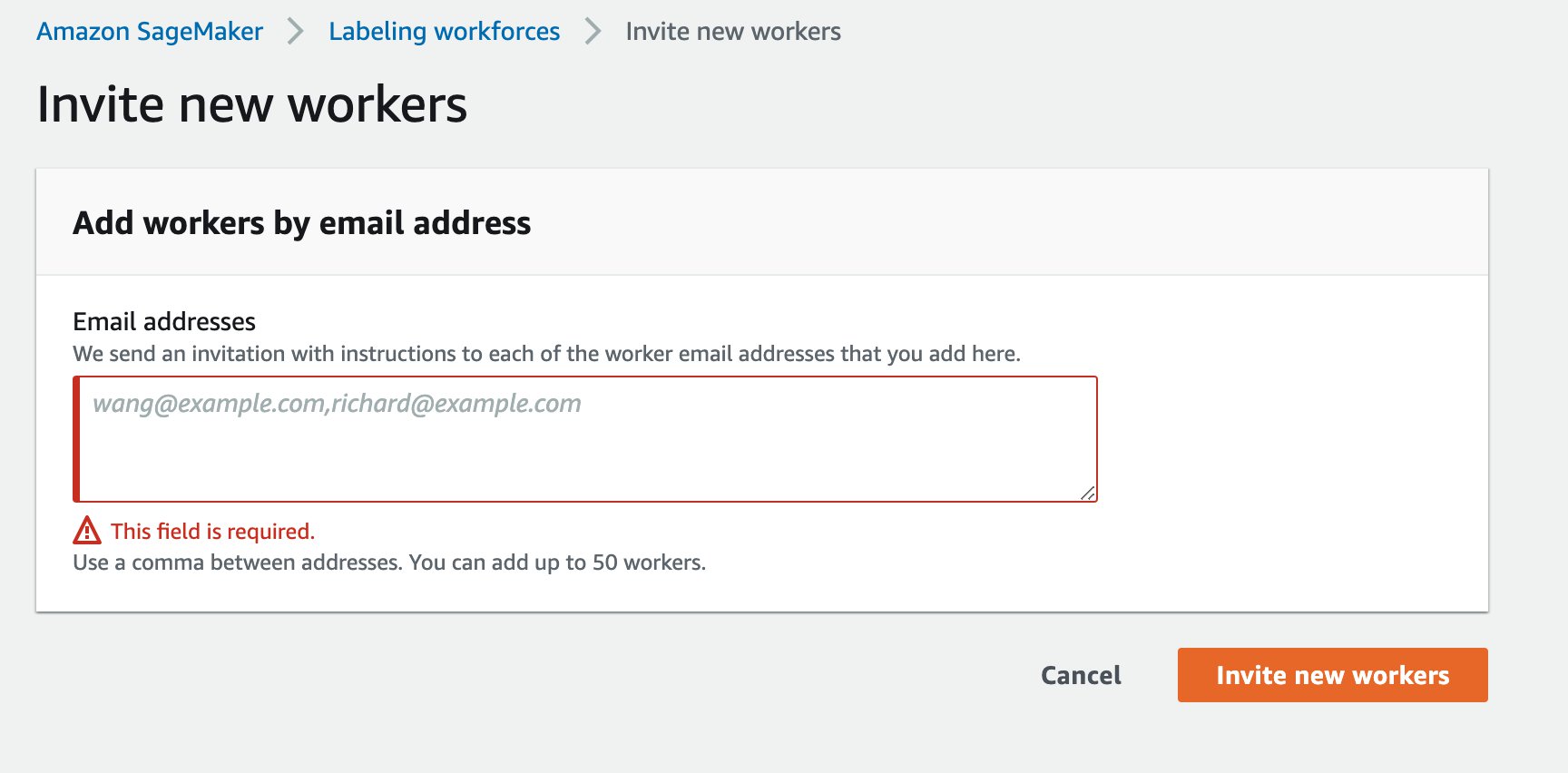
After you add the worker, they receive an email, similar to the one shown in the following screenshot.

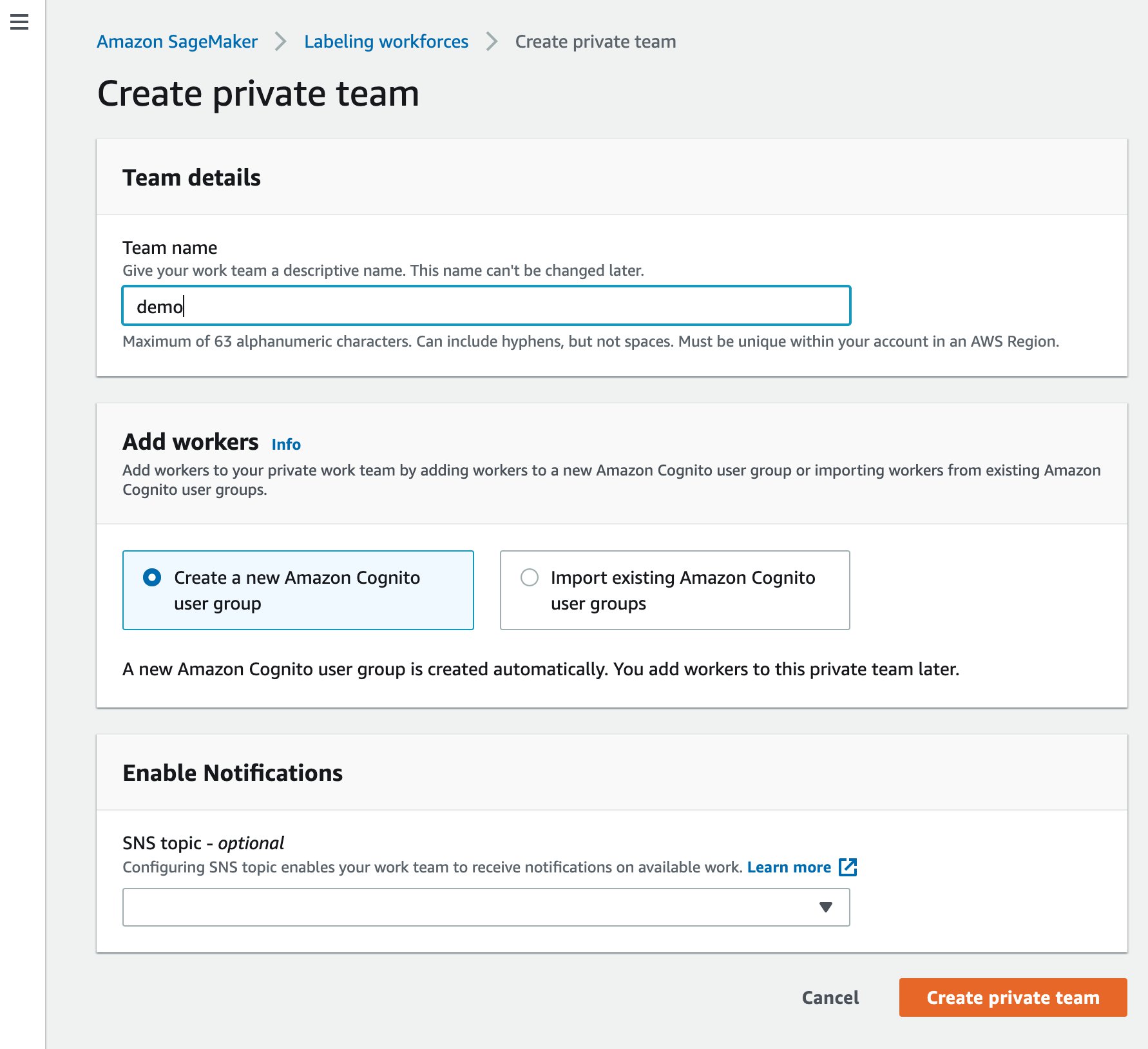
Meanwhile, you can create a new labeling team.
- Choose Create private team.
- For Team name, enter a name.
- Choose Create private team to confirm.
- On the Labeling workforces page, choose the name of the team.
- On the Workers tab, choose Add workers to team.
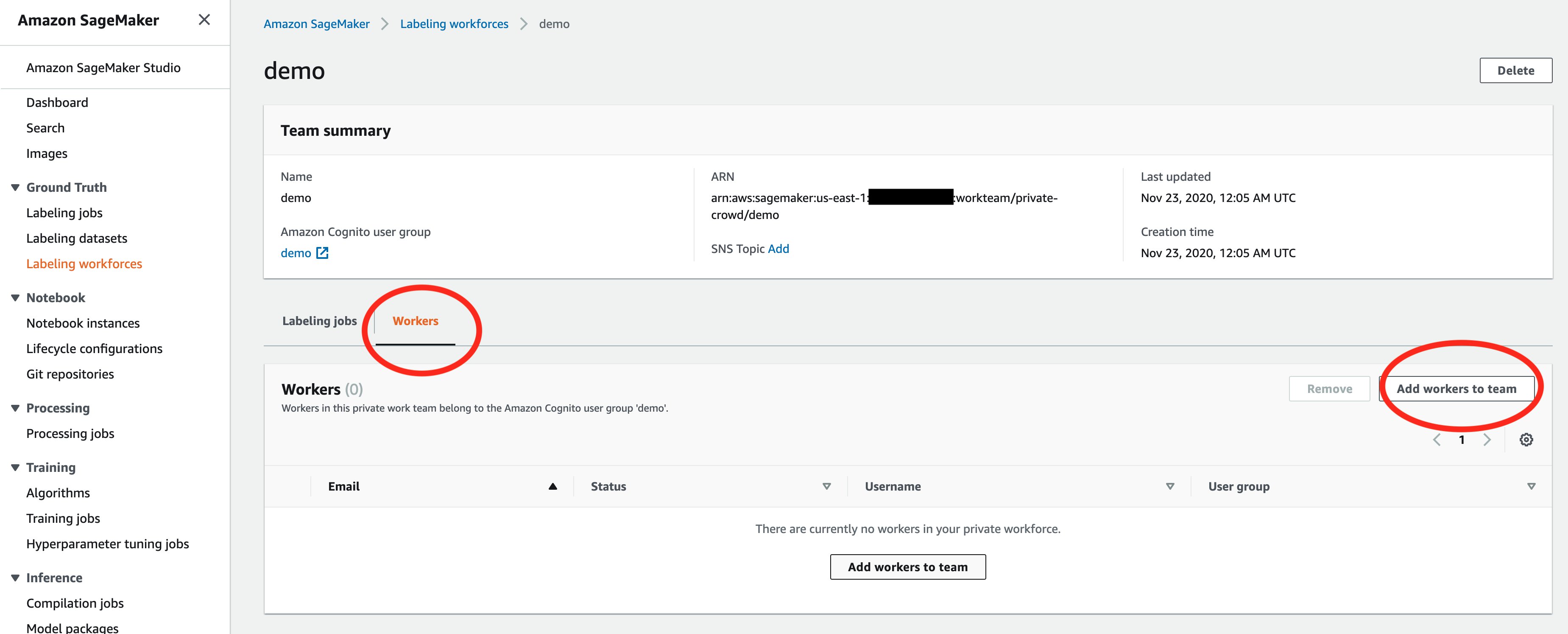
- Select the intended worker’s email address and choose Add workers to team.

Finally, we can get the labeling workforce ARN. For more details, see Create and Manage Workforces.
Deploy the CloudFormation stack
Deploy the CloudFormation stack in one of the AWS Regions where you are going to use Amazon Rekognition Custom Labels. This solution is currently available in us-east-1 (N. Virginia) and eu-west-1 (Ireland).
| Region | Launch |
| US East (N. Virginia) | |
| EU West (Ireland) | |
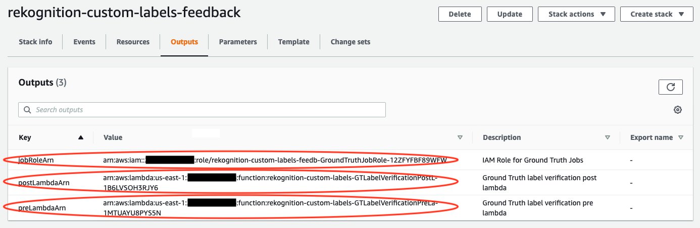
After deployment, choose the Outputs tab and make note of the three outputs: jobRoleArn, preLambdaArn, and postLambdaArn.
Train the first version of your model
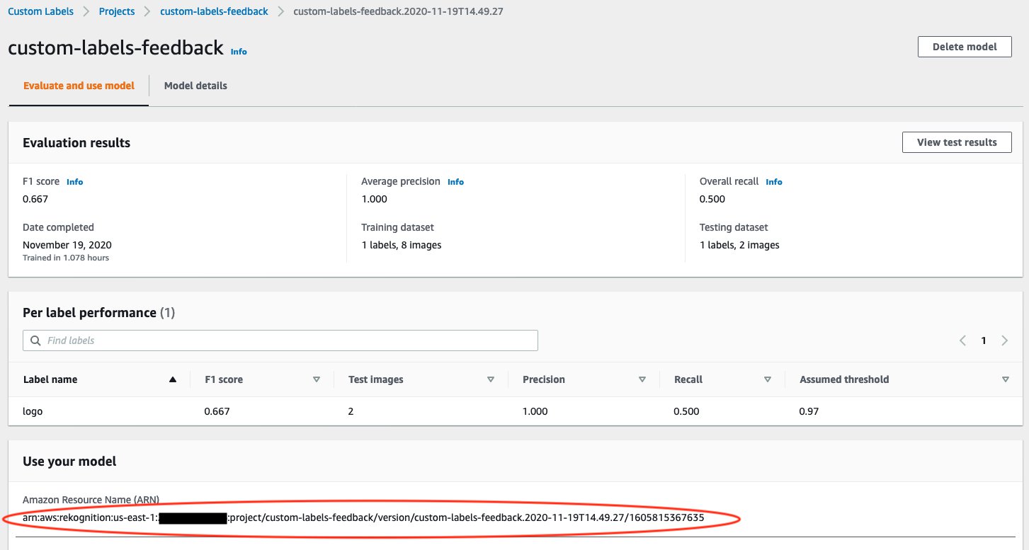
For instructions on creating a project and training a model with Custom Labels, see Announcing Amazon Rekognition Custom Labels. In this post, we create a project called custom-labels-feedback. The first version model was trained and validated using the v1 dataset that includes eight AWS or Amazon smile logo images. The following screenshot shows some labeled sample data used for training.

When the first version model’s training process is finished, take note of your model ARN. In our example, the model performance achieved an F1 score as 0.667. We use this model to help human workers to annotate a larger dataset (v2) for the next iteration.
Start the feedback client
To start the feedback client, complete the following steps:
- In your terminal, clone the repository:
git clone https://github.com/aws-samples/amazon-rekognition-custom-labels-feedback-solution.git- Change the working directory:
cd amazon-rekognition-custom-labels-feedback-solution/src- Update the following items in
feedback-config.jsonin thesrc/ folder:- images – The S3 bucket folder that has the larger dataset. In this post, it is the v2 dataset that contains 30 images.
- outputBucket – The output S3 bucket. For best practices, we recommend using the same image bucket here.
- jobRoleArn – The output from the CloudFormation stack.
- workforceTeamArn – The private team ARN as set earlier in the Ground Truth labeling workforces.
- preLambdaArn – The output from the CloudFormation stack.
- postLambdaArn – The output from the CloudFormation stack.
- projectVersionArn – The first model ARN.

You need to start the first version model before you call the feedback client.
- Expand the API Code section on your Amazon Rekognition Custom Labels model page, and enter the AWS CLI command
Start modelin your terminal.

The model status changes to STARTING.
- When the model status changes to RUNNING, run the following code in your terminal:
python3 start-feedback.pyIt analyzes the larger dataset of images using the first version model and starts Ground Truth label verification jobs. It also outputs a command for later usage, which generates a manifest file for the larger dataset (v2).

Perform label verification
Now human workers can log in the labeling project to verify labels proposed by the first version model. Usually, label verification jobs are sent to the workers in several batches.

For most of the images that are labeled correctly by the first version model, human workers only need to confirm these labels without any adjustment, which accelerates the whole data annotation process.

Generate a manifest file for the second dataset
After the label verification jobs are complete, (the status of the labeling jobs in Ground Truth changes from In progress to Complete), run the following command that you got from the feedback client’s output in your terminal:
python3 get-feedback.py --jobs-manifest s3://......This command generates a manifest file for the larger dataset that you can use to train the next version of your model in Rekognition Custom Labels. The output S3 Path indicates the manifest file location for the larger dataset.

Train the second version of your model
To train the next version of your model, we first create a new dataset.
- On the Amazon Rekognition Custom Labels console, choose Create dataset.
- For Dataset name, enter a name.
- For Image location, select Import images labeled by Amazon SageMaker Ground Truth.
- For .manifest file location, enter the S3 path you noted earlier.

Double check whether all images are labeled correctly. The following screenshot shows some sample data that we imported from Ground Truth.

With this newly added dataset in Amazon Rekognition Custom Labels, you can train the next version of your model under the same project as the first version. For example, in this post, we train the next version model using the dataset amazon-logo-v2 under the project custom-labels-feedback, and use the dataset amazon-logo-v1 as a test set.

In our example, comparing to the first version, the next version model achieves much better performance with a 0.900 F1 score.

It’s worth noting that you can apply this solution multiple times in a Amazon Rekognition Custom Labels project. You can use the next version model to easily annotate even larger datasets and train models until you’re satisfied with final model performance.
Clean up
After you finish using the custom labels feedback solution, remember to delete the CloudFormation stack via the AWS CloudFormation console, and stop running models by calling the AWS CLI command in your terminal. This helps you avoid any unnecessary charges.
Conclusion
This post presented an end-to-end demonstration of using Amazon Rekognition Custom Labels to efficiently annotate a larger dataset with assistance from a model trained on a smaller dataset. This solution enables you to gain feedback on a model’s performance and make improvements by using human verification and adjustment when necessary. As a result, data annotation, model training, and error analysis are conducted simultaneously and interactively, which improves dataset annotation efficiency.
For more information about building dataset labels with Ground Truth, see Amazon SageMaker Ground Truth and Amazon Rekognition Custom Labels.
About the Authors
 Sherry Ding is a Senior AI/ML Specialist Solutions Architect. She has extensive experience in machine learning with a PhD degree in Computer Science. She mainly works with Public Sector customers on various AI/ML related business challenges, helping them accelerate their machine learning journey on the AWS Cloud. When not helping customers, she enjoys outdoor activities.
 Kashif Imran is a Principal Solutions Architect at Amazon Web Services. He works with some of the largest AWS customers who are taking advantage of AI/ML to solve complex business problems. He provides technical guidance and design advice to implement computer vision applications at scale. His expertise spans application architecture, serverless, containers, NoSQL, and machine learning.
 Dr. Baichuan Sun is a Senior Data Scientist at AWS AI/ML. He is passionate about solving strategic business problems with customers using data-driven methodology on the cloud, and he has been leading projects in challenging areas including robotics computer vision, time series forecasting, price optimization, predictive maintenance, pharmaceutical development, product recommendation system, etc. In his spare time he enjoys traveling and hanging out with family
Smart city traffic anomaly detection using Amazon Lookout for Metrics and Amazon Kinesis Data Analytics Studio
Cities across the world are transforming their public services infrastructure with the mission of enhancing the quality of life of its residents. Roads and traffic management systems are part of the central nervous system of every city. They need intelligent monitoring and automation in order to prevent substantial productivity loss and in extreme cases life-threatening situations such as obstruction to free movement of emergency services.
Today, in most city traffic operations centers, monitoring video feeds from roadside cameras is a fairly manual activity. It requires operations center engineers to mentally correlate and apply institutional knowledge to determine if an ongoing situation is an anomaly, which makes this activity error-prone and susceptible to delays.

Where AI/ML based solutions have been applied to analyze video feeds, there is a lot of complexity involved in ingesting, curating, and preparing data in the right format and then optimizing and maintaining the effectiveness of these machine learning (ML) models over long periods of time. This has been one of the barriers to quickly implementing and scaling the adoption of ML capabilities and in turn realizing the automation outcomes at city traffic operation centers.
This post shows you how to use an integrated solution with Amazon Lookout for Metrics and Amazon Kinesis Data Analytics Studio (among other AWS services) to break these barriers by quickly and easily ingesting streaming data, aggregating and curating it, and subsequently detecting anomalies in the key performance indicators of your interest.
Lookout for Metrics automatically detects and diagnoses anomalies (outliers from the norm) in business and operational data. It’s a fully managed ML service, which uses specialized ML models to detect anomalies based on the characteristics of your data. You don’t need ML experience to use Lookout for Metrics.
Kinesis Data Analytics Studio provides an interactive notebook experience powered by Apache Zeppelin and Apache Flink to analyze streaming data. It also helps productionize your analytics application by building and deploying code as a Kinesis data analytics application straight from the notebook.
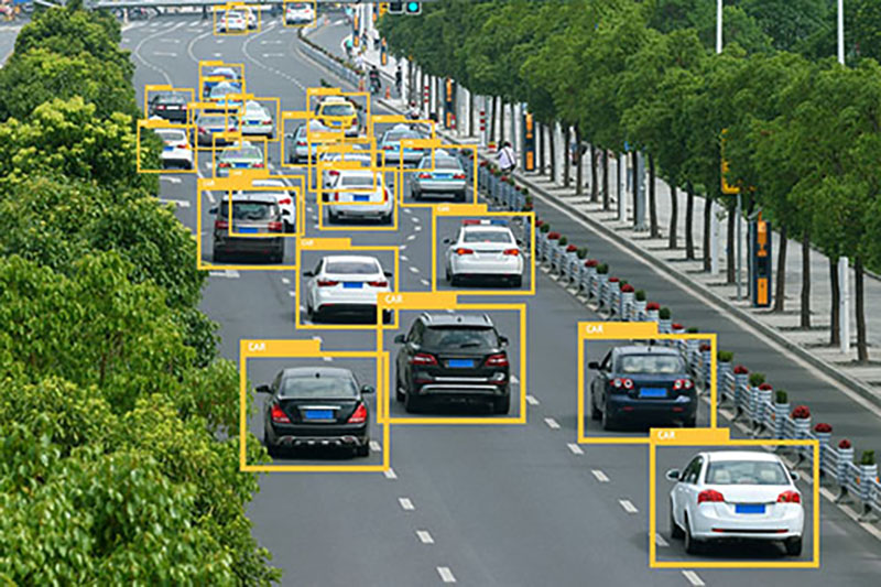
We demonstrate one of the most common traffic management scenarios, in which we detect anomalies in the number of vehicles and persons passing the view of ML-capable video infrastructure deployed at the roadside in order to enable capabilities such as automated traffic light pattern optimization, dynamic utilization of reserved lanes, and rapid deployment of emergency services. By the end of this post, you’ll learn how to use these managed services from AWS to meet the outcomes of smart cities to increase safety and reduce traffic. This solution can be equally applied to accelerate other outcomes for smart city management such as detecting anomalies in water supply (water pipe leaks), crowd density (safe campuses in the context of the pandemic), non-green energy usage, and community Wi-Fi traffic patterns, to name a few.
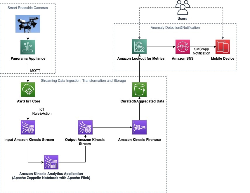
Solution architecture
The architecture consists of three functional blocks:
- Smart roadside cameras
- Streaming data ingestion, transformation, and storage
- Anomaly detection and notification
The solution provides a fully automated data path from the smart cameras all the way to a notification being raised to the user. You can also interact with the solution using the Lookout for Metrics UI in order to analyze the identified anomalies.
The following diagram illustrates our solution architecture.
Smart roadside cameras using AWS Panorama
Data can be ingested from traffic cameras in several ways. The most optimal way is to analyze the video feed using computer vision ML algorithms instead of transporting thousands of video streams to the cloud and then running ML algorithms there. AWS released a computer vision appliance called AWS Panorama at AWS re:Invent 2020; it’s an ML appliance and software development kit (SDK) that allows you to bring computer vision to on-premises cameras to make predictions locally with high accuracy and low latency. AWS Panorama is well suited to address the use case of traffic monitoring. One AWS Panorama Appliance can ingest and analyze video streams from multiple video cameras. You can deploy a multi-object tracking ML model on the AWS Panorama Appliance to identify and track the vehicles passing by the camera. You can install AWS Panorama Appliances in sheltered cabinets in large road junctions or in cabinets by the roadside to cover a section of the road.
You can also send the inference results to AWS IoT Core to further process the data and make business decisions based on your requirements.
Because this post focuses on anomaly detection of traffic patterns, we assume that the AWS Panorama Appliance is already sending inference results to AWS IoT Core. In the subsequent sections, we focus on how the streaming data is processed from AWS IoT Core and analyzed to detect anomalies.
For more information, see AWS IoT and Building and deploying an object detection computer vision application at the edge with AWS Panorama.
Streaming data ingestion and transformation using Amazon Kinesis
Data from IoT devices is usually in the form of a continuous time series data stream. This is data that usually must be processed sequentially and incrementally on a record-by-record basis or over sliding time windows, and can be used for a variety of analytics, including correlations, aggregations, filtering, and sampling.
AWS IoT integrates with Amazon Kinesis Data Streams, which is a fully managed streaming data integration service. By default, the streaming data is available for 24 hours. This streaming data is then queried and transformed using a Kinesis data analytics application, which is built and deployed using Kinesis Data Analytics Studio. For more information, see Introducing Amazon Kinesis Data Analytics Studio – Quickly Interact with Streaming Data Using SQL, Python, or Scala.
We show you in the subsequent sections how to use Kinesis Data Analytics Studio, Kinesis Data Streams, and Amazon Kinesis Data Firehose to ingest traffic data from the IoT-powered smart cameras, transform it in real time using Flink SQL, and then deliver the data to an Amazon Simple Storage Service (Amazon S3) bucket in a custom prefix pattern that is compatible with Lookout for Metrics. It’s easy to build this data pipeline with minimal code. Also, because all the AWS services involved in the data pipeline are managed services, you can focus on enhancing functionality rather than running and maintaining infrastructure.
Anomaly detection using Lookout for Metrics
Lookout for Metrics automatically inspects and prepares the data dropped into Amazon S3 to detect anomalies with greater speed and accuracy than traditional methods used for anomaly detection. As anomalies are detected, you can provide feedback on detected anomalies to tune the results and improve accuracy over time. Lookout for Metrics makes it easy to diagnose detected anomalies by grouping anomalies that are related to the same event and sending an alert that includes a summary of the potential root cause. It also ranks anomalies in order of severity so you can prioritize your attention to what matters most to your business.
In the subsequent sections, we dive deep into configuring Amazon Kinesis services and Lookout for Metrics.
Prerequisites
To follow along and test this solution yourself, you need the following prerequisites:
- An AWS account
- The AWS Command Line Interface (AWS CLI) installed on your machine
- An AWS Panorama Appliance along with a smart camera or a MQTT message simulator that can provide data in the described JSON format
- An introductory level of knowledge of AWS IoT, AWS Glue, and Kinesis Data Analytics
Data ingestion and transformation using AWS IoT and Kinesis
We use Kinesis Data Streams to ingest the streaming data from AWS IoT Core. We create two streams: one for the source data and another for the transformed data.
The following AWS CLI command creates the input stream:
$ aws kinesis create-stream
--stream-name traffic-data-stream
--shard-count 1
--region eu-central-1
The following AWS CLI command creates the output stream:
$ aws kinesis create-stream
--stream-name processed-traffic-stream
--shard-count 1
--region eu-central-1
Let’s look at the data coming in from the AWS Panorama Appliance. You can view the inferred data from the multi-object tracking model by running a test on the AWS IoT console by providing the IoT topic where the inferences of the model are published. The data the you receive is in JSON format and shows the object detected and a unique ID for the appearance of a particular person or car in the region of interest of the camera. A snippet of the data is as follows:
{
  "person": <person id>
}
{
  "car": <car id>
}
Now we create an AWS IoT Core rule to send the incoming data from the AWS Panorama Appliance to the Kinesis data stream. We limit the data to persons and cars, and include a timestamp using the following query in the AWS IoT rule definition. Inclusion of the timestamp is mandatory for anomaly detection.
SELECT person,car,timestamp() as event_time FROM <IOT topic>We also add an action as part of the rule definition to send the data selected to the input data stream we created previously.
At this point, we have data from the AWS Panorama Appliance streaming into our traffic-data-stream stream.
Now let’s create a Kinesis Data Analytics studio to analyze the data streaming in. We create the notebook of type Apache Flink, which allows us to analyze the data using SQL. You need to either create a new AWS Glue database or use an existing one to store the table definitions for the incoming and outgoing data streams. For detailed steps for creating an Apache Zeppelin notebook, see Introducing Amazon Kinesis Data Analytics Studio – Quickly Interact with Streaming Data Using SQL, Python, or Scala or Using a Studio notebook with Kinesis Data Analytics for Apache Flink.
After we create the notebook, we create a new note and call it traffic-anomaly-data-transformer. This should provide you an interactive environment to write your code (see the following screenshot).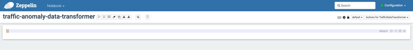
Enter the following SQL statement to create a table for the traffic data source:
%flink.ssql
create TABLE traffic_data_source (
    person FLOAT,
    car FLOAT,
    event_time AS PROCTIME()
)
PARTITIONED BY (person)
WITH (
    'connector' = 'kinesis',
    'stream' = 'traffic-data-stream',
    'aws.region' = 'eu-central-1',
    'scan.stream.initpos' = 'LATEST',
    'format' = 'json'
);
The first part of the SQL statement uses %flink.ssql to tell Apache Zeppelin to provide a stream SQL environment for the Apache Flink interpreter.
The second part describes the connector used to receive data in the table (for example, Kinesis or Kafka), the name of the stream, the AWS Region, and the overall data format of the stream (such as JSON or CSV). We can also choose the starting position to process the stream; we use LATEST to read the most recent data first.
Now let’s create a table for the traffic data destination as follows:
%flink.ssql
CREATE TABLE traffic_data_dest (
    person BIGINT,
    car    BIGINT,
    hop_time TIMESTAMP(3)
)
WITH (
'connector' = 'kinesis',
'stream' = 'processed-traffic-stream',
'aws.region' = 'eu-central-1',
'scan.stream.initpos' = 'LATEST',
'format' = 'json'
);
Next, we run the following query, which counts the number of persons and cars seen in a window of 5 minutes and inserts that data into the traffic_data_dest data stream:
%flink.ssql(type=update)
INSERT INTO traffic_data_dest
SELECT COUNT(person) AS person,COUNT(car) AS car,
       TUMBLE_END(event_time, INTERVAL '5' minute) as tumble_time
  FROM traffic_data_source
 GROUP BY TUMBLE(event_time, INTERVAL '5' minute);
In the preceding code, we use the TUMBLE_END function to record the timestamp on the record sent to the data stream as the end of the 5-minute window rather than the start of the window. This is important later in the post, when we assign custom prefix names in Amazon S3 based on time intervals—using TUMBLE_END ensures that the timestamp on the record and the prefix name are for the same 5-minute interval.
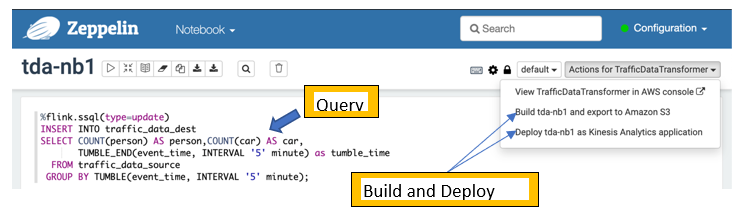
After this is successful, deploy this query as a Kinesis data analytics application. To do this, we add a new note called tda-nb1 (short for “traffic data application, notebook 1”) and copy only the preceding SQL statement that queries data from the source stream and inserts it into the destination stream. We don’t need to copy the create table SQL statements because the tables have already been created in AWS Glue.
The Apache Zeppelin notebook provides a fully automated deployment capability at the push of a button. You perform two steps: build and export the code to an S3 bucket of your choice, and deploy the code as a Kinesis data analytics application.
One important step is to update the AWS Identity and Access Management (IAM) roles of the Kinesis data analytics application in order to access the source data stream, destination data stream, and the AWS Glue Data Catalog.
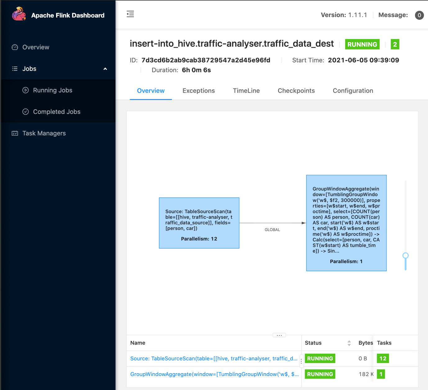
We now run the application. We should see the application graph (as in the following screenshot) showing the data flow from source to destination, and you should be able to open the Apache Flink dashboard to get more information about the application run.
We now create a Kinesis Data Firehose delivery stream that reads from the processed-traffic-data stream (output stream) and delivers the data to Amazon S3. One of the key points to note is the configuration of the custom prefix that is configured for the Amazon S3 destination. This prefix pattern ensures that the data is created in the S3 bucket as per the prefix hierarchy expected by Lookout for Metrics. (More on this later in this post.) For more information about custom prefixes for S3 objects, see Custom Prefixes for Amazon S3 Objects.
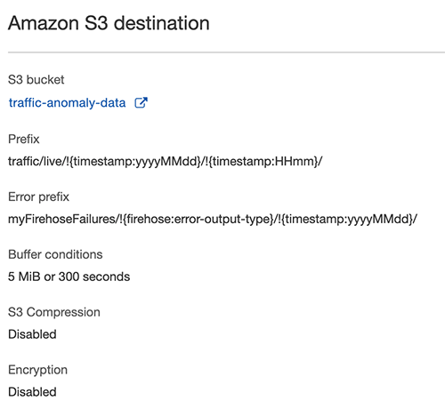
As shown in the following screenshot, the data is delivered to the specified S3 bucket in the prefix structure.
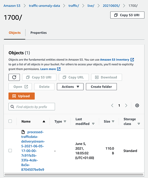
The data within one of the files is as follows:
{"person":12,"car":56,"hop_time":"2021-06-05T16:55:00"}
{"person":15,"car":121,"hop_time":"2021-06-05T17:00:00"}
The timestamps show that each file contains data for two 5-minute intervals.
With minimal code, we have now ingested the data from the camera, created a durable input stream from the ingested data, transformed the data based on the metrics we want to measure (the number of cars and persons), and stored the data in an S3 bucket based on the requirements for Lookout for Metrics.
In the following section, we take a deeper look at the constructs within Lookout for Metrics.
Lookout for Metrics deep dive
Let’s look at the terms and concepts within Lookout for Metrics, how they apply to this use case, and how easy it is to configure these concepts using the Lookout for Metrics console.
Detector
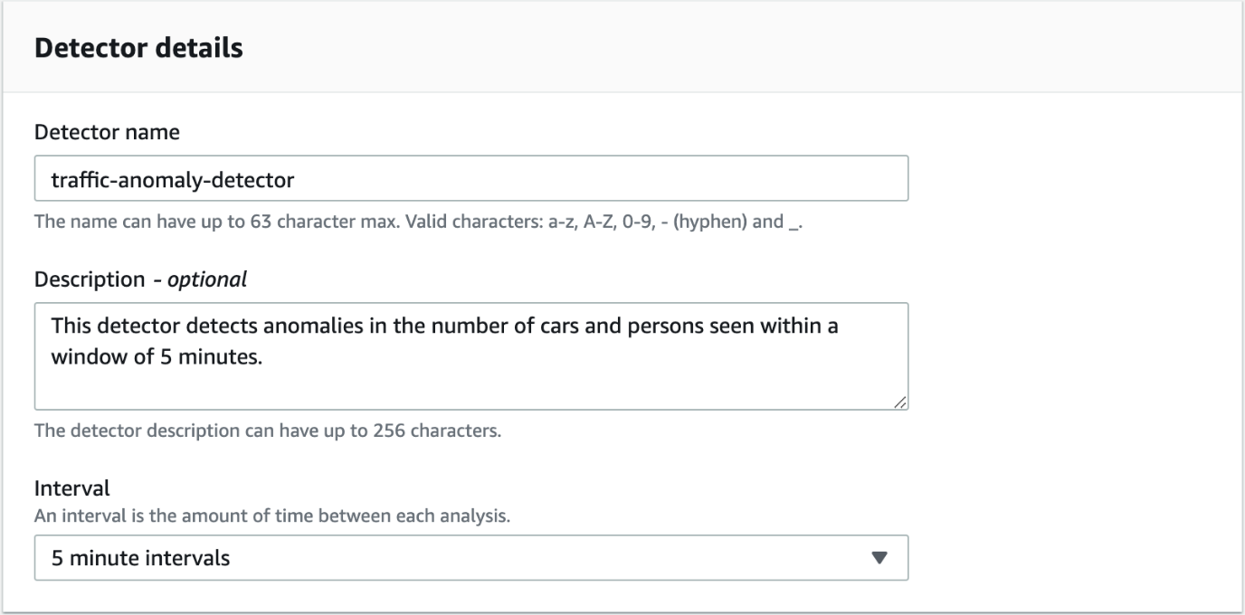
A detector is a Lookout for Metrics resource that monitors a dataset and identifies anomalies at a predefined frequency. Detectors use ML to find patterns in data and distinguish between expected variations in data and legitimate anomalies. To improve its performance, a detector learns more about your data over time.
In our use case, the detector analyzes aggregated data from the camera every 5 minutes. To create the detector, navigate to the Lookout for Metrics console and choose Create Detector. Provide the name and description (optional) for the detector, along with the interval of 5 minutes.
Your data is encrypted by default with a key that AWS owns and manages for you. You can also configure if you want to use a different encryption key from the one that is used by default.
Now, let’s point this detector to the data that you want it to run anomaly detection on.
Dataset
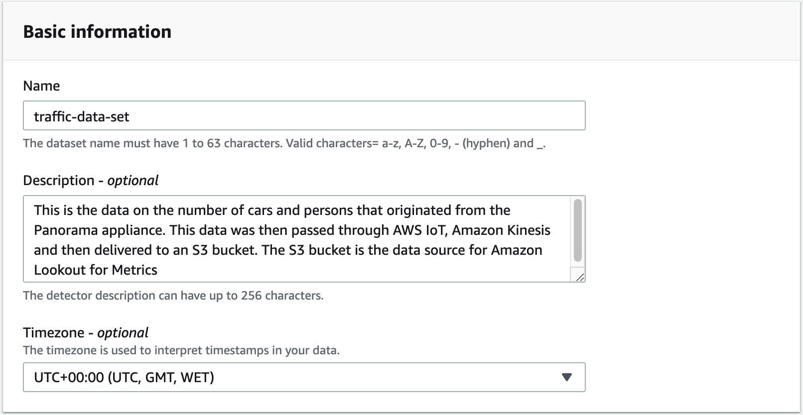
A dataset tells the detector where to find your data and which metrics to analyze for anomalies.
We create the dataset on the Amazon Lookout for Metrics console, and provide a name (for this post, traffic-data-set), description (optional), and time zone.
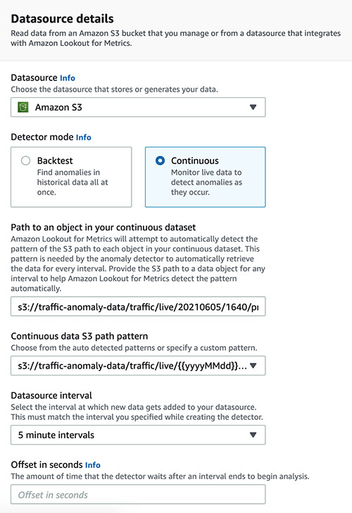
In our use case, we choose Amazon S3 as our data source. With Amazon S3, you can create a detector in two modes:
- Backtest – This mode is used to find anomalies in historical data. It needs all records to be consolidated in a single file.
- Continuous – This mode is used to detect anomalies in live data. We use this mode with our use case because we want to detect anomalies as we receive traffic data from the roadside camera. The rest of this post talks about configuring continuous mode.
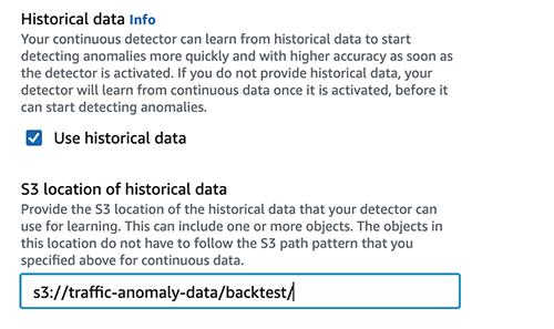
The path where the live data lands every 5 minutes is configured. As explained in the data ingestion and transformation section, the data is stored in the following folder structure.
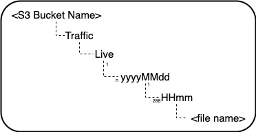
The details of the S3 prefix path and the folder structure is configured as shown in the following screenshot.
If there is a delay in the data ingestion into Amazon S3, you can define an offset in seconds that defines the time the detector waits before it runs the anomaly analysis for a particular interval.
Also, if you have historical data from which the detector can learn patterns, you can provide it during this configuration. The data here is expected to be in the same format that you use to perform a backtest. Providing historical data speeds up the ML model training process. If this isn’t available, the continuous detector waits for sufficient data to be available before making inferences.
You can specify additional configurations to help Lookout for Metrics understand the format of the data that you are analyzing. Also, you must specify the IAM role that is used by Lookout for Metrics to access the data source.
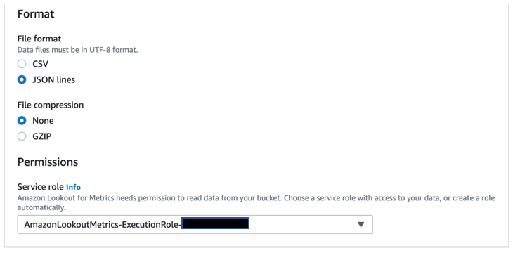
At this point, Lookout for Metrics accesses the data source and validates whether it can parse the data. If the parsing is successful, it gives you a “Validation successful” message and takes you to the next screen, where you configure measures, dimensions, and timestamps.
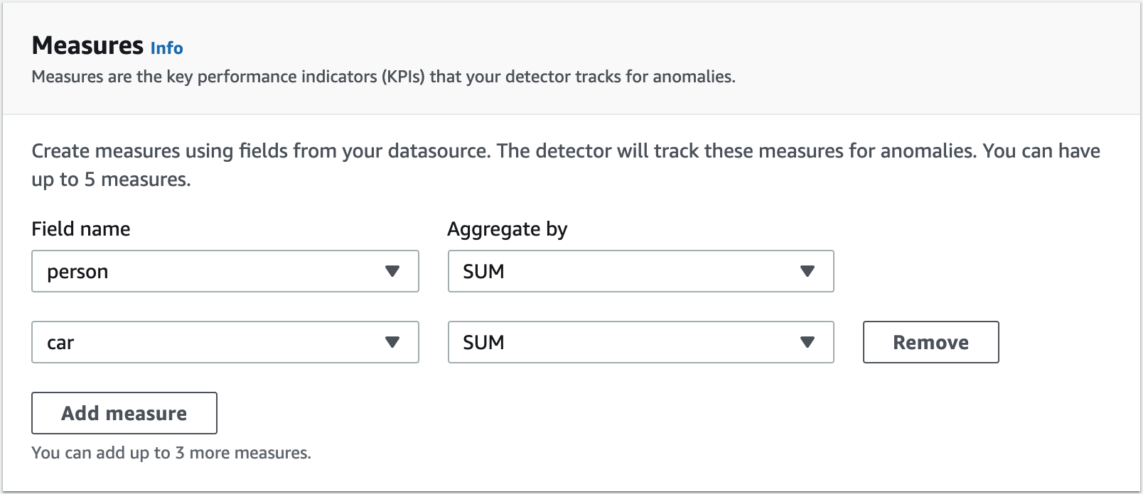
Measures, dimensions and timestamps
Measures define KPIs that you want to track anomalies for. You can add up to five measures per detector. The fields that are used to create KPIs from your source data must be of numeric format. The KPIs can be currently defined by aggregating records within the time interval by doing a SUM or AVERAGE.
In our use case, we add one measure, which does the SUM of the objects seen in the 5-minute interval.
Dimensions give you the ability to slice and dice your data by defining categories or segments. This allows you to track anomalies for a subset of the whole set of data for which a particular measure is applicable.
In our use case, we have only one camera feeding data to the solution. Imagine if we had all the cameras from the city connected. Then we could use the camera ID or other metadata such as locality name as dimensions.
Every record in the dataset must have a timestamp. The following configuration allows you to choose the field that represents the timestamp value and also the format of the timestamp.
The next screen allows you to review all the details you have added and then save and activate the detector.
The detector then begins learning the data streaming into the data source. At this stage, the status of the detector changes to Initializing.
It’s important to note the minimum amount of data that is required before which Lookout for Metrics can start detecting anomalies. For more information about requirements and limits, see Lookout for Metrics quotas.
Fantastic! With minimal configuration, you have created your detector, pointed it at a dataset, and defined the metrics that you want Lookout for Metrics to find anomalies in.
Anomaly visualization
Lookout for Metrics provides a rich UI experience for users who want to use the AWS Management Console to analyze the anomalies being detected. It also provides the capability to query the anomalies via API.
Let’s look at an example anomaly detected from our traffic data use case.
The following screenshot shows an anomaly detected in the count of cars at the said time and date with a severity score of 100. It also shows the percentage contribution of the dimension towards the anomaly. In this case, 100% contribution comes from the car dimension.
Further down the page, you also get a line graph of the metric, along with the ability to view the metric data across time periods of the previous 30 minutes, 1 hour, 2 hours, 6 hours, or the maximum number of intervals. The anomaly is highlighted in blue on the graph.
As the service detects anomalies, it also allows you to provide human feedback to specify whether the detected anomaly is relevant. In our scenario, because the number of cars suddenly increased to 87 from 1, it was highlighted as an anomaly as compared to previous data, and we confirmed that by choosing Yes.
Alerts
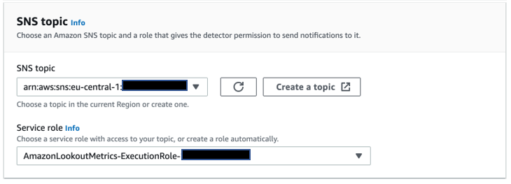
Lookout for Metrics allows you to send alerts using a variety of channels. You can configure the anomaly severity score threshold at which the alerts must be triggered.
In our use case, we configure alerts to be sent to an Amazon Simple Notification Service (Amazon SNS) channel, which in turn sends an SMS.
You can also use an alert to trigger automations using AWS Lambda functions in order to drive API-driven operations on AWS IoT Core. You can use IoT device shadows to control display devices in order to control traffic signals or traffic lane sign boards. If a rapid action team of personnel needs to be deployed, we could imagine the alert triggering a workforce management system that selects and deploys available personnel to the site to deal with the emergency.
Conclusion
Cities have the opportunity to derive insights from traffic management systems and make better decisions to improve public safety, make daily commutes less frustrating, and improve the overall quality of life of its residents.
In this post, we showed you how to use Lookout for Metrics and Kinesis to remove the undifferentiated heavy lifting involved in managing the end-to-end lifecycle of building ML-powered anomaly detection applications.
We believe that this solution will truly help you accelerate your ability to find anomalies in key business metrics and allow you focus your efforts on growing and improving your business.
We encourage you to learn more by visiting the Amazon Lookout for Metrics Developer Guide and Using a Studio notebook with Kinesis Data Analytics for Apache Flink, and also try out the end-to-end solution enabled by these services with the dataset relevant to your business KPIs.
We’re eager and excited to see what you’ll build using Amazon Lookout for Metrics and Amazon Kinesis Data Analytics Studio in the context of smart cities and beyond.
About the Authors
 Ajay Ravindranathan is a Sr Partner Solutions Architect with Amazon Web Services, and is passionate about helping customers build modern applications using AWS services. Ajay has a keen interest in building AI/ML powered cloud-native products that can help telecommunications service providers on their digital transformation journey.
 Bala KP is a Sr Partner Solutions Architect with Amazon Web Services. He works with partners and customers in the financial services and insurance domain to provide them with architecture guidance on building scalable and secure applications in AWS.
New take on hierarchical time series forecasting improves accuracy
Method enforces “coherence” of hierarchical time series, in which the values at each level of the hierarchy are sums of the values at the level below.Read More
Shopping Smart: AiFi Using AI to Spark a Retail Renaissance
Walk into a store. Grab your stuff. And walk right out again, without stopping to check out.
In just the past three months, California-based AiFi has helped Choice Market increase sales at one of its Denver stores by 20 percent among customers who opted to skip the checkout line.
It allowed Żabka, a Polish convenience store chain, to provide faster checkout for morning train commuters.
It helped pro-racing team Penske and Verizon run a dinky 200-square-foot store at the Indy500, so race fans could quickly get back to the action.
And on Wednesday AiFi announced an expanded partnership with Loop Neighborhood to introduce its computer vision, camera-only platform into stores in California, starting with two Bay Area locations.
AiFi, a member of the NVIDIA Inception accelerator for AI and deep learning startups, has moved out of the proof-of-concept stage and into stores across the world.
Its technology makes shopping more convenient and helps retailers better understand their customers.

“Retailers can now get as much information about physical shopping habits as online stores are getting from ecommerce,” said AiFi CEO and co-founder Steve Gu, a veteran of Apple and Google.
AiFi’s ability to analyze shopper habits is even more impressive because its stores don’t need to buy costly sensors and RFID tags.
Instead, the company uses real-time image recognition and edge AI powered by NVIDIA GPUs to recognize the items shoppers select and charge them, usually through an app linked to the customer’s credit card.
It’s not an easy task in busy stores stocked with many hundreds of items, but the five-year-old company’s technology now achieves an accuracy rate of 99 percent.
To date, more than 15 stores worldwide are putting the company’s technology to work. Those stores are already serving satisfied customers who return again and again.
At Choice Market, 60 percent of shoppers who tried the checkout-free option used it again within a month. Twenty percent came back three times.
The computer-vision-powered system uses NVIDIA Metropolis for smart video analytics. It works smoothly alongside the store’s traditional checkout system, and is integrated with the Choice Now app, where customers can shop checkout-free, and place online orders and arrange pickups.
AiFi is revolutionizing retail operations with AI. At the Indy500 auto race earlier this year, Penske Entertainment’s nano-store allowed fans to buy snacks, beverages and merchandise with an app. No need to stop and swipe a credit card.
This speed translates well to any kind of store where people need to slip in and out in a hurry. Żabka partnered with AiFi to open its first public autonomous store in Poznan, Poland, quickly drawing huge amounts of foot traffic from commuters going to and from a nearby train station.
With AiFi integrated with the Żappka App, which has over 5 million users, harried commuters could hustle out the door with a newspaper and a morning coffee.

More stores equipped with AiFi’s technology are coming. In France, the company is working with Carrefour on what the retailer calls its “Flash LabStore,” a frictionless store at its headquarters in Massy.
And in the UK, Britain’s fourth-largest supermarket, Morrisons, is working with AiFi to test out a store with no checkout.
These stores represent a growing number of collaborations with major retailers that see AiFi’s combination of AI and computer vision as the key to a brick and mortar retail renaissance that will ultimately put more goods in front of more customers, in more places.
Learn more about NVIDIA’s AI platform powering intelligent retail stores.
The post Shopping Smart: AiFi Using AI to Spark a Retail Renaissance appeared first on The Official NVIDIA Blog.
Use Amazon SageMaker Feature Store in a Java environment
Feature engineering is a process of applying transformations on raw data that a machine learning (ML) model can use. As an organization scales, this process is typically repeated by multiple teams that use the same features for different ML solutions. Because of this, organizations are forced to develop their own feature management system.
Additionally, you can also have a non-negotiable Java compatibility requirement due to existing data pipelines developed in Java, supporting services that can only be integrated with Java, or in-house applications that only expose Java APIs. Creating and maintaining such a feature management system can be expensive and time-consuming.
In this post, we address this challenge by adopting Amazon SageMaker Feature Store, a fully managed, purpose-built repository to securely store, update, retrieve, and share ML. We use Java to create a feature group; describe and list the feature group; ingest, read, and delete records from the feature group; and lastly delete the feature group. We also demonstrate how to create custom utility functions such as multi-threaded ingest to meet performance requirements. You can find the code used to build and deploy this solution into your own AWS account in the GitHub repo.
| For more details about Feature Store and different use cases, see the following: |
Credit card fraud use case
In our example, Organization X is a finance-tech company and has been combating credit card fraudulence for decades. They use Apache frameworks to develop their data pipelines and other services in Java. These data pipelines collect, process, and transform raw streaming data into feature sets. These feature sets are then stored in separated databases for model training and inference. Over the years, these data pipelines have created a massive number of feature sets and the organization doesn’t have a system to properly manage them. They’re looking to use Feature Store as their solution.
To help with this, we first configure a Java environment in an Amazon SageMaker notebook instance. With the use of a synthetic dataset, we walk through a complete end-to-end Java example with a few extra utility functions to show how to use Feature Store. The synthetic dataset contains two tables: identity and transactions. The transaction table contains the transaction amount and credit or debit card, and the identity table contains user and device information. You can find the datasets on GitHub.
Differences between Boto3 SDK and Java SDK
Each AWS service, including SageMaker, exposes an endpoint. An endpoint is the URL of the entry point for an AWS offering. The AWS SDKs and AWS Command Line Interface (AWS CLI) automatically use the default endpoint for each service in an AWS Region, but you can specify an alternate endpoint for your API requests.
You can connect directly to the SageMaker API or to the SageMaker Runtime through HTTPs implementations. But in that case, you have to handle low-level implementation details such as credentials management, pagination, retry algorithms (adaptive retry, disable retries), logging, debugging, error handling, and authentication. Usually these are handled by the AWS SDK for Python (Boto3), a Python-specific SDK provided by SageMaker and other AWS services.
The SDK for Python implements, provides, and abstracts away the low-level implementational details of querying an endpoint URL. While doing this, it exposes important tunable parameters via configuration parameters. The SDK implements elemental operations such as read, write, delete, and more. It also implements compound operations such as bulk read and bulk write. The definition of these compound operations is driven by your specific need; in the case of Feature Store, they’re provided in the form of bulk ingest.
Sometimes organizations can also have a non-negotiable Java compatibility requirement for consumption of AWS services. In such a situation, the AWS service needs to be consumed via the AWS SDK for Java and not via SDK for Python. This further drives the need to compose these compound functions using Java and reimplement the SDK for Python functionality using the SDK for Java.
Set up a Java environment
In this section, we describe the setup pattern for the Java SDK.
To help set up this particular example without too much hassle, we prefer using SageMaker notebooks instance as a base from which to run these examples. SageMaker notebooks are available in various instance types; for this post, an inexpensive instance such as ml.t3.medium suffices.
Perform the following commands in the terminal of the SageMaker notebook instance to confirm the Java version:
sh-4.2$ java --version
openjdk 11.0.9.1-internal 2020-11-04
OpenJDK Runtime Environment (build 11.0.9.1-internal+0-adhoc..src)
OpenJDK 64-Bit Server VM (build 11.0.9.1-internal+0-adhoc..src, mixed mode)
Next, install Maven:
cd /opt
sudo wget https://apache.osuosl.org/maven/maven-3/3.6.3/binaries/apache-maven-3.6.3-bin.tar.gz
sudo tar xzvf apache-maven-3.6.3-bin.tar.gz
export PATH=/opt/apache-maven-3.6.3/bin:$PATH
Finally, clone our repository from GitHub, which includes code and the pom.xml to set up this example.
After the repository is cloned successfully, run this example from within the Java directory:
mvn compile; mvn exec:java -Dexec.mainClass="com.example.customername.FeatureStoreAPIExample"Java end-to-end solution overview
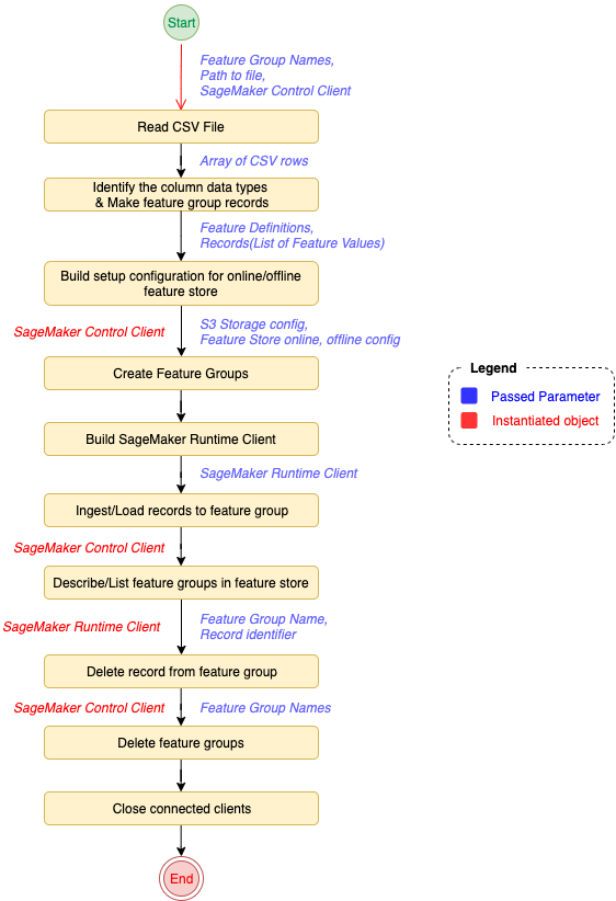
After the environment is fully configured, we can start calling the Feature Store API from Java. The following diagram workflow outlines the end-to-end solution for Organization X for their fraud detection datasets.
Configure the feature store
To create the feature groups that contain the feature definitions, we first need to define the configurations for the online and offline feature store into which we ingest the features from the dataset. We also need to set up a new Amazon Simple Storage Service (Amazon S3) bucket to use as our offline feature store. Then, we initialize a SageMaker client using an ARN role with the proper permissions to access both Amazon S3 and the SageMaker APIs.
The ARN role that you use must have the following managed policies attached to it: AmazonSageMakerFullAccess and AmazonSageMakerFeatureStoreAccess.

The following code snippet shows the configuration variables that need to be user-specified in order to establish access and connect to the Amazon S3 client, SageMaker client, and Feature Store runtime client:
public static void main(String[] args) throws IOException {

  // Specify the region for your env
  static final Region REGION = Region.US_EAST_1;

  //S3 bucket where the Offline store data is stored
  // Replace with your value
  static final String BUCKET_NAME = "YOUR_BUCKET_NAME";

  // Replace with your value
  static final String FEATURE_GROUP_DESCRIPTION = "YOUR_DESCRIPTION";

  // Replace with your value
  static final String SAGEMAKER_ROLE_ARN = "YOUR_SAGEMAKER_ARN_ROLE";

  // CSV file path
  static final String FILE_PATH = "../data/Transaction_data.csv";

  // Feature groups to create
  static final String[] FEATURE_GROUP_NAMES = {
    "Transactions"
  };

  // Unique record identifier name for feature group records
  static final String RECORD_IDENTIFIER_FEATURE_NAME = "TransactionID";

  // Timestamp feature name for Feature Store to track
  static final String EVENT_TIME_FEATURE_NAME = "EventTime";

  // Number of threads to create per feature group ingestion, or can be
  // determined dynamically through custom functions
  static final int NUM_OF_THREADS = 4;

  // Utility function which contains the feature group API operations
featureGroupAPIs(
    BUCKET_NAME, FILE_PATH, FEATURE_GROUP_NAMES,
    RECORD_IDENTIFIER_FEATURE_NAME, EVENT_TIME_FEATURE_NAME,
    FEATURE_GROUP_DESCRIPTION, SAGEMAKER_ROLE_ARN, NUM_OF_THREADS, REGION);

  System.exit(0);
};
We have now set up the configuration and can start invoking SageMaker and Feature Store operations.
Create a feature group
To create a feature group, we must first identify the types of data that exist in our dataset. The identification of feature definitions and the data types of the features occur during this phase, as well as creating the list of records in feature group ingestible format. The following steps don’t have to occur right after the initial data identification, but in our example, we do this at the same time to avoid parsing the data twice and to improve overall performance efficiency.
The following code snippet loads the dataset into memory and runs the identification utility functions:
// Read csv data into list
List < String[] > csvList = CsvIO.readCSVIntoList(filepath);

// Get the feature names from the first row of the CSV file
String[] featureNames = csvList.get(0);

// Get the second row of data for data type inferencing
String[] rowOfData = csvList.get(1);

// Initialize the below variable depending on whether the csv has an idx
// column or not
boolean isIgnoreIdxColumn = featureNames[0].length() == 0 ? true : false;

// Get column definitions
List < FeatureDefinition > columnDefinitions =
    FeatureGroupRecordOperations.makeColumnDefinitions(
        featureNames, rowOfData, EVENT_TIME_FEATURE_NAME, isIgnoreIdxColumn);

// Build and create a list of records
List < List < FeatureValue >> featureRecordsList =
    FeatureGroupRecordOperations.makeRecordsList(featureNames, csvList,
        isIgnoreIdxColumn, true);
After we create the list of feature definitions and feature values, we can utilize these variables for creation of our desired feature group and ingest the data by establishing connections to the controlling SageMaker client, Feature Store runtime client, and by building the online and offline Feature Store configurations.
The following code snippet demonstrates the setup for our creation use case:
S3StorageConfig s3StorageConfig =
    S3StorageConfig.builder()
        .s3Uri(
            String.format("s3://%1$s/sagemaker-featurestore-demo/",
            BUCKET_NAME))
        .build();

OfflineStoreConfig offlineStoreConfig =
    OfflineStoreConfig.builder()
        .s3StorageConfig(s3StorageConfig)
        .build();

OnlineStoreConfig onlineStoreConfig =
    OnlineStoreConfig.builder()
        .enableOnlineStore(Boolean.TRUE)
        .build();

SageMakerClient sageMakerClient =
    SageMakerClient.builder()
        .region(REGION)
        .build();

S3Client s3Client =
    S3Client.builder()
        .region(REGION)
        .build();

SageMakerFeatureStoreRuntimeClient sageMakerFeatureStoreRuntimeClient =
    SageMakerFeatureStoreRuntimeClient.builder()
        .region(REGION)
        .build();
We develop and integrate a custom utility function with the SageMaker client to create our feature group:
// Create feature group
FeatureGroupOperations.createFeatureGroups(
    sageMakerClient, FEATURE_GROUP_NAMES, FEATURE_GROUP_DESCRIPTION,
    onlineStoreConfig, EVENT_TIME_FEATURE_NAME, offlineStoreConfig,
    columnDefinitions, RECORD_IDENTIFIER_FEATURE_NAME,
    SAGEMAKER_ROLE_ARN);
For a deeper dive into the code, refer to the GitHub repo.
After we create a feature group and its state is set to ACTIVE, we can invoke API calls to the feature group and add data as records. We can think of records as a row in a table. Each record has a unique RecordIdentifier and other feature values for all FeatureDefinitions that exist in the FeatureGroup.
Ingest data into the feature group
In this section, we demonstrate the code incorporated into the utility function we use to multi-thread a batch ingest to our created feature group using the list of records (FeatureRecordsList) that we created earlier in the feature definition identification step:
// Total number of threads to create for batch ingestion
static final int NUM_OF_THREADS_TO_CREATE =
    NUM_OF_THREADS * FEATURE_GROUP_NAMES.length;

// Ingest data from csv data
Ingest.batchIngest(
    NUM_OF_THREADS_TO_CREATE, sageMakerFeatureStoreRuntimeClient,
    featureRecordsList, FEATURE_GROUP_NAMES, EVENT_TIME_FEATURE_NAME);
During the ingestion process, we should see the ingestion progress on the console as status outputs. The following code is the output after the ingestion is complete:
Starting batch ingestion
Ingest_0 is running
Ingest_1 is running
Ingest_2 is running
Number of created threads: 4
Ingest_3 is running
Thread: Ingest_2 => ingested: 500 out of 500
Thread: Ingest_2, State: TERMINATED
Thread: Ingest_1 => ingested: 500 out of 500
Thread: Ingest_1, State: TERMINATED
Thread: Ingest_0 => ingested: 500 out of 500
Thread: Ingest_0, State: TERMINATED
Thread: Ingest_3 => ingested: 500 out of 500
Thread: Ingest_3, State: TERMINATED
Ingestion finished
Ingested 2000 of 2000
Now that we have created the desired feature group and ingested the records, we can run several operations on the feature groups.
List and describe a feature group
We can list and describe the structure and definition of the desired feature group or of all the feature groups in our feature store by invoking getAllFeatureGroups() on the SageMaker client then calling describeFeatureGroup() on the list of feature group summaries that is returned in the response:
// Invoke the list feature Group API
List < FeatureGroupSummary > featureGroups =
    FeatureGroupOperations.getAllFeatureGroups(sageMakerClient);

// Describe each feature Group
FeatureGroupOperations.describeFeatureGroups(sageMakerClient, featureGroups);
The preceding utility function iterates through each of the feature groups and outputs the following details:
Feature group name is: Transactions

Feature group creation time is: 2021-04-28T23:24:54.744Z

Feature group feature Definitions is:
[
    FeatureDefinition(FeatureName=TransactionID, FeatureType=Integral),
    FeatureDefinition(FeatureName=isFraud, FeatureType=Integral),
    FeatureDefinition(FeatureName=TransactionDT, FeatureType=Integral),
    FeatureDefinition(FeatureName=TransactionAmt, FeatureType=Fractional),
    FeatureDefinition(FeatureName=card1, FeatureType=Integral),
    FeatureDefinition(FeatureName=card2, FeatureType=Fractional),
…
    FeatureDefinition(FeatureName=card_type_0, FeatureType=Integral),
    FeatureDefinition(FeatureName=card_type_credit, FeatureType=Integral),
    FeatureDefinition(FeatureName=card_type_debit, FeatureType=Integral),
    FeatureDefinition(FeatureName=card_bank_0, FeatureType=Integral),
    FeatureDefinition(FeatureName=card_bank_american_express, FeatureType=Integral),
    FeatureDefinition(FeatureName=card_bank_discover, FeatureType=Integral),
    FeatureDefinition(FeatureName=card_bank_mastercard, FeatureType=Integral),
    FeatureDefinition(FeatureName=card_bank_visa, FeatureType=Integral),
    FeatureDefinition(FeatureName=EventTime, FeatureType=Fractional)
]

Feature group description is: someDescription
Retrieve a record from the feature group
Now that we know that our features groups are populated, we can fetch records from the feature groups for our fraud detection example. We first define the record that we want to retrieve from the feature group. The utility function used in this section also measures the performance metrics to show the real-time performance of the feature store when it’s used to train models for inference deployments. See the following code:
// Loop getRecord for FeatureGroups in our feature store
static final int AMOUNT_TO_REPEAT = 1;
static final String RECORD_IDENTIFIER_VALUE = "2997887";
FeatureGroupOperations.runFeatureGroupGetTests(
    sageMakerClient, sageMakerFeatureStoreRuntimeClient, featureGroups,
    AMOUNT_TO_REPEAT, RECORD_IDENTIFIER_VALUE);
You should see the following output from the record retrieval:
Getting records from feature group: Transactions
Records retrieved: 1 out of: 1
Retrieved record feature values:
[
    FeatureValue(FeatureName=TransactionID, ValueAsString=2997887),
    FeatureValue(FeatureName=isFraud, ValueAsString=1),
    FeatureValue(FeatureName=TransactionDT, ValueAsString=328678),
    FeatureValue(FeatureName=TransactionAmt, ValueAsString=13.051),
    FeatureValue(FeatureName=card1, ValueAsString=2801),
    FeatureValue(FeatureName=card2, ValueAsString=130.0),
    FeatureValue(FeatureName=card3, ValueAsString=185.0),
…
    FeatureValue(FeatureName=card_type_0, ValueAsString=0),
    FeatureValue(FeatureName=card_type_credit, ValueAsString=1),
    FeatureValue(FeatureName=card_type_debit, ValueAsString=0),
    FeatureValue(FeatureName=card_bank_0, ValueAsString=0),
    FeatureValue(FeatureName=card_bank_american_express, ValueAsString=0),
    FeatureValue(FeatureName=card_bank_discover, ValueAsString=0),
    FeatureValue(FeatureName=card_bank_mastercard, ValueAsString=0),
    FeatureValue(FeatureName=card_bank_visa, ValueAsString=1),
    FeatureValue(FeatureName=EventTime, ValueAsString=1619655284.177000)
]
Delete a record from the feature group
The deleteRecord API call deletes a specific record from the list of existing records in a specific feature group:
// Delete record with id 2997887
FeatureGroupOperations.deleteRecord(
    sageMakerFeatureStoreRuntimeClient, FEATURE_GROUP_NAMES[0],
    RECORD_IDENTIFIER_VALUE);
The preceding operation should log the following output with status 200, showing that the delete operation was successful:
Deleting record with identifier: 2997887 from feature group: Transactions
Record with identifier deletion HTTP response status code: 200
Although feature store is used for ongoing ingestion and update of the features, you can still remove the feature group after the fraud detection example use case is over in order to save costs, because you only pay for what you provision and use with AWS.
Delete the feature group
Delete the feature group and any data that was written to the OnlineStore of the feature group. Data can no longer be accessed from the OnlineStore immediately after DeleteFeatureGroup is called. Data written into the OfflineStore is not deleted. The AWS Glue database and tables that are automatically created for your OfflineStore are not deleted. See the following code:
// Delete featureGroups
FeatureGroupOperations.deleteExistingFeatureGroups(
    sageMakerClient, FEATURE_GROUP_NAMES);
The preceding operation should output the following to confirm that deletion has properly completed:
Deleting feature group: Transactions
...
Feature Group: Transactions cannot be found. Might have been deleted.

Feature group deleted is: Transactions
Close connections
Now that we have completed all the operations on the feature store, we need to close our client connections and stop the provisioned AWS services:
sageMakerFeatureStoreRuntimeClient.close();
sageMakerClient.close();
s3Client.close();
Conclusion
In this post, we showed how to configure a Java environment in a SageMaker instance. We walked through an end-to-end example to demonstrate not only what Feature Store is capable of, but also how to develop custom utility functions in Java, such as multi-threaded ingestion to improve the efficiency and performance of the workflow.
To learn more about Amazon SageMaker Feature Store, check out this overview of its key features. It is our hope that this post, together with our code examples, can help organizations and Java developers integrate Feature Store into their services and application. You can access the entire example on GitHub. Try it out, and let us know what you think in the comments.
About the Authors
 Ivan Cui is a Data Scientist with AWS Professional Services, where he helps customers build and deploy solutions using machine learning on AWS. He has worked with customers across diverse industries, including software, finance, pharmaceutical, and healthcare. In his free time, he enjoys reading, spending time with his family, and maximizing his stock portfolio.
 Chaitanya Hazarey is a Senior ML Architect with the Amazon SageMaker team. He focuses on helping customers design, deploy, and scale end-to-end ML pipelines in production on AWS. He is also passionate about improving explainability, interpretability, and accessibility of AI solutions.
 Daniel Choi is an Associate Cloud Developer with AWS Professional Services, who helps customers build solutions using the big data analytics and machine learning platforms and services on AWS. He has created solutions for clients in the AI automated manufacturing, AR/MR, broadcasting, and finance industries utilizing his data analytics specialty whilst incorporating his SDE background. In his free time, he likes to invent and build new IoT home automation devices and woodwork.
 Raghu Ramesha is a Software Development Engineer (AI/ML) with the Amazon SageMaker Services SA team. He focuses on helping customers migrate ML production workloads to SageMaker at scale. He specializes in machine learning, AI, and computer vision domains, and holds a master’s degree in Computer Science from UT Dallas. In his free time, he enjoys traveling and photography.
Prepare and clean your data for Amazon Forecast
You might use traditional methods to forecast future business outcomes, but these traditional methods are often not flexible enough to account for varying factors, such as weather or promotions, outside of the traditional time series data considered. With the advancement of machine learning (ML) and the elasticity that the AWS Cloud brings, you can now enjoy more accurate forecasts that influence business decisions. You will learn how to interpret and format your data according to what Amazon Forecast needs based on your business questions.
This post shows you how to prepare your data to optimally use with Amazon Forecast. Amazon Forecast is a fully managed service that allows you to forecast your time series data with high accuracy. It uses ML to analyze complex relationships in historical data and doesn’t require any prior ML experience. With its deep integration capabilities with the AWS Cloud, your forecasting process can be fully automated and highly flexible.
We will begin by understanding the different types of input data that Forecast accepts. With a retail use case, we will discuss how to structure your data to match the use case and forecasting granularity of the business metric that you are interested in forecasting. Then, we will discuss how to clean your data and handle challenging scenarios, such as missing values, to generate the most accurate forecasts.
Factors affecting forecast accuracy
Amazon Forecast uses your data to train a private, custom model tailored to your use case. ML models are only as good as the data put into them, and it’s important to understand what the model needs. Amazon Forecast can accept three types of datasets: target time series, related time series, and item metadata. Amongst those, target time series is the only mandatory dataset. This historical data provides the majority of the model’s accuracy.
Amazon Forecast provides predefined dataset domains that specify a schema of what data to include in which input datasets for common use cases, such as forecasting for retail, web traffic, and more. The domains are convenient column names only. The underlying models aren’t affected by these column names because they’re dropped prior to training. For the remainder of this post, we use the retail domain as an example.
Target time series data
Target time series data defines the historical demand for the resources you’re predicting. As mentioned earlier, the target time series dataset is mandatory. It contains three required fields:
- item_id – Describes a unique identifier for the item or category you want to predict. This field may be named differently depending on your dataset domain (for example, in the workforce domain this is
workforce_type, which helps distinguish different groups of your labor force). - timestamp – Describes the date and time at which the observation was recorded.
- demand – Describes the amount of the item, specified by
item_id, that was consumed at the timestamp specified. For example, this could be the number of pink shoes sold on a certain day.
You can also add additional fields in your input data. For example, in the retail dataset domain, you can optionally add an additional field titled location. This can help to add context about where the consumption occurred for that record and forecast the demand for items on a per-store basis where multiple stores are selling the same item. The best practice is to create a concatenated item_id identifier that includes product and location identifiers. One exception to this rule is if you know more than string names of locations, such as “Store 1”. If you know actual geolocations, such as postal codes or latitude/longitude points, then geolocation data such as weather can be pulled in automatically. This geolocation field needs to be separate from the item_id.
The frequency of your observations in the historical data you provide is also important, because it dictates the frequency of your forecasts that can be generated. You can provide target time series data with fine granularity such as a per-minute frequency, where historical demand is recorded every minute, up to as wide of a granularity as a yearly frequency. The data granularity must be smaller than or equal to your desired forecast granularity. If you want predictions on a monthly basis for each item, you should input data with monthly or finer granularity. The granularity shouldn’t be larger than your desired forecast frequency (for example, giving yearly observations in historical data when you want forecasts on a monthly basis).
High-quality datasets consist of dense data where there is almost a data point for every item and timestamp. Sparse data doesn’t give Amazon Forecast enough information to determine historical patterns to forecast with. To achieve accurate forecasts, ensure that you can supply dense data or fill in missing data points with null filling, as described later in this post.
Related time series data
In addition to historical sales data, other data may be known per item at exactly the same time as every sale. This data is called related time series data. Related data can give more clues to what future predictions could look like. The best related data is also known in the future. Examples of related data include prices, promotions, economic indicators, holidays, and weather. Although related time series data is optional, including additional information can help increase accuracy by providing context of various conditions that may have affected demand.
The related time series dataset must include the same dimensions as the target time series, such as the timestamp and item_id. Additionally, you can include up to a maximum of 13 related features. For more information about useful features you may want to include for different use cases, see Predefined Dataset Domains and Dataset Types.
Amazon Forecast trains a model using all input data. If the related time series doesn’t improve accuracy, it’s not used. When training with related data, it’s best to train using the CNN-QR algorithm, if possible, then check the model parameters to see if your related time series data was useful for improving accuracy.
Item metadata
Providing item metadata to Amazon Forecast is optional, but can help refine forecasts by adding contextual information about items that appear in your target time series data. Item metadata is static information that doesn’t change with time, describing features about items such as the color and size of a product being sold. Amazon Forecast uses this data to create predictions based on similarities between products.
To use item metadata, you upload a separate file to Amazon Forecast. Each row in the CSV file you upload must contain the item ID, followed by the metadata features for that item. Each row can have a maximum of 10 fields, including the field that contained the item ID.
Item metadata is required when forecasting demand for an item that has no historical demand, known as the cold start problem. This could be a new product that you want to launch, for example. Because item metadata is required, demand for new products can’t be forecasted except if your data qualifies to train a deep learning algorithm. By understanding the demand of items with similar features, Amazon Forecast predicts demand for your new product. For more information about forecasting for cold start scenarios, see the following best practices on GitHub.
Now that you understand the different types of input data and their formats, we explore how to manipulate your data to achieve your business objectives.
Structure your input data based on your business questions
When preparing your input data for Amazon Forecast, consider the business questions you want to ask. As mentioned earlier, Amazon Forecast requires three mandatory input columns (timestamp, item_id, and value) as part of your time series data. You need to prepare your input data by applying aggregations to your input data while keeping the eventual structure in line to the input format. The following scenarios explain how you can manipulate and prepare your input data depending on your business questions.
Imagine we have the following dataset showing your daily sales per product. In this example, your company is selling two different products (Product A and Product B) in different stores (Store 1 and Store 2) across two different countries (Canada and the US).
| Date | Product ID | Sales | Store ID | Country |
| 01-Jan | Product A | 3 | Store-1 | Canada |
| 01-Jan | Product B | 5 | Store-1 | Canada |
| 01-Jan | Product A | 4 | Store-2 | US |
| 02-Jan | Product A | 4 | Store-2 | US |
| 02-Jan | Product B | 3 | Store-2 | US |
| 02-Jan | Product A | 2 | Store-1 | Canada |
| 03-Jan | Product B | 1 | Store-1 | Canada |
The granularity of the provided sales data is on a per-store, country, item ID, and per-day basis. This initial assessment is useful when we prepare the data for the input.
Now imagine you need to ask the following forecasting question: “How many sales should I anticipate for Product A on January 4?”
The question is looking for an answer for a particular day, so you need to tell Amazon Forecast to predict at a daily frequency. Amazon Forecast can produce the forecasts at the desired daily frequency because the raw data is reported at the same granularity level or less.
The question also asks for a specific product, Product A. Because the raw data reports sales on a per-product granularity already, no further data preparation action is required for product aggregation.
The source data shows that sales are reported per store. Because we’re not interested in forecasting on a per-store basis, you need to aggregate all the sales data of each product across all the stores.
Taking these into account, your Amazon Forecast input structure looks like the following table.
| timestamp | item_id | demand |
| 01-Jan | Product A | 7 |
| 01-Jan | Product B | 5 |
| 02-Jan | Product A | 6 |
| 02-Jan | Product B | 3 |
| 03-Jan | Product B | 1 |
Another business question you might ask could be: “How many sales should I anticipate from Canada on January 4?”
In this question, the granularity is still daily, so Amazon Forecast can produce daily forecasts. The question doesn’t ask for a specific product or store. However, it asks for a prediction on a country level. The source data shows that the data is broken down on a per-store basis, and each store has one-to-one mapping to a country. That means you need to sum up all sales across all the different stores within the same country.
Your Amazon Forecast input structure looks like the following table.
| timestamp | item_id | demand |
| 01-Jan | Canada | 8 |
| 01-Jan | US | 4 |
| 02-Jan | Canada | 2 |
| 02-Jan | US | 7 |
| 03-Jan | Canada | 1 |
Lastly, we ask the following question: “How much overall sales should I anticipate for February?”
This question doesn’t mention any dimensions other than time. That means that all the sales data should be aggregated across all products, stores, and countries per month. Because Amazon Forecast requires a specific date to use as the timestamp, you can use the first of each month to indicate a month’s aggregated demand. Your Amazon Forecast input structure looks like the following table.
| timestamp | item_id | demand |
| 01-Jan | daily | 22 |
This example data is just for demonstration purposes. Real-life datasets should be much larger, because a larger historical dataset yields more accurate predictions. For more information, see the data size best practices on GitHub. Remember that while you’re doing aggregations across dimensions, you’re reducing the total number of input data points. If there is little historical data, aggregation leads to fewer input data points, which may not be enough for Amazon Forecast to accurately train your predictor. You can experiment with different aggregation levels within your data and explore how they affect the accuracy of your predictions through iteration.
Data cleaning
Cleaning your data for Amazon Forecast is important because it can affect the accuracy of the forecasts that are created. To demonstrate some best practices, we use the Department store sales and stocks dataset provided by the Government of Canada. The data is already prepared for Amazon Forecast to predict on a monthly basis for each unique department using historical data from January 1991 to December 1997. The following table shows an excerpt of the cleaned data.
| REF_DATE | Type of department | VALUE |
| 1991-01 | Bedding and household linens | 37150 |
| 1991-02 | Bedding and household linens | 31470 |
| 1991-03 | Bedding and household linens | 34903 |
| 1991-04 | Bedding and household linens | 36218 |
| 1991-05 | Bedding and household linens | 40453 |
| 1991-06 | Bedding and household linens | 42204 |
| 1991-07 | Bedding and household linens | 48364 |
| 1991-08 | Bedding and household linens | 47920 |
| 1991-09 | Bedding and household linens | 44887 |
| 1991-10 | Bedding and household linens | 45551 |
In the following sections, we describe some of the steps that were taken to understand and cleanse our data.
Visualize the data
Previously, we discussed how granularity of data dictates forecast frequency and how you can manipulate data granularity to suit your business questions. With visualization, you can see at what levels of time and product granularity your data exhibits smoother patterns, which give the ML model better inputs for learning. If your data appears to be intermittent or sparse, try to aggregate data into a higher granularity (for example, aggregating all sales for a given day as a single data point) with equally spaced time intervals. If your data has too few observations to determine a trend over time, your data has been aggregated at too high a level and you should reduce the granularity to a finer level. For sample Python code, see our Data Prep notebook.
In the following chart of yearly demand for bedding and household items, we visualize the data from earlier at the yearly aggregation level. The chart shows a one-time bump in the year 1994 that isn’t repeated. This is a bad aggregation level to use because there is no repeatable pattern to the historical sales. In addition, yearly aggregation results in too little historical data, which isn’t enough for Amazon Forecast to use.

Next, we can visualize our sample dataset at a monthly granularity level to identify patterns in our data. In the following figure, we plotted data for the bedding and household items department and added a trendline. We can observe a seasonal trend that is predictable, which Amazon Forecast can learn and predict with.

Handle missing and zero values
You must also be careful of gaps and zero values within your target time series data. If the target field value (such as demand) is zero for a timestamp and item ID combination, this could mean that data was simply missing, the item wasn’t in stock, and so on. Having zeroes in your data that aren’t actual zeroes, such as values representing new or end-of-life products, can bias a model toward zero. When preparing your data, one best practice is to convert all zero values to null and let Amazon Forecast do the heavy lifting by automatically detecting new products and end-of-life products. In addition, adding an out-of-stock related variable per item_id and timestamp can improve accuracy. When you replace zeroes with null values, they’re replaced according to the filling logic you specify, which you can change based on your null filling strategy.
In our sample dataset, the data for the plumbing, heating, and building materials department is blank or contains a 0 after June 1993.
| timestamp | item_id | demand |
| 1991-01-01 | Plumbing, heating and building materials | 5993 |
| 1991-02-01 | Plumbing, heating and building materials | 4661 |
| 1991-03-01 | Plumbing, heating and building materials | 5826 |
| … | … | … |
| 1993-05-01 | Plumbing, heating and building materials | 5821 |
| 1993-06-01 | Plumbing, heating and building materials | 6107 |
| … | … | … |
| 1993-07-01 | Plumbing, heating and building materials | |
| 1993-08-01 | Plumbing, heating and building materials | |
| 1993-09-01 | Plumbing, heating and building materials | |
| …. | …. | …. |
| 1995-11-01 | Plumbing, heating and building materials | |
| 1995-12-01 | Plumbing, heating and building materials | 0 |
| 1996-01-01 | Plumbing, heating and building materials | 0 |
| 1996-02-01 | Plumbing, heating and building materials | 0 |
Upon further inspection, only blank and zero values are observed until the end of the dataset. This is known as the end-of-life problem. We have two options: simply remove these items from training data because we know that their forecast should be zero, or replace all zeroes with nulls and let Amazon Forecast automatically detect end-of-life products with null filling logic.
Conclusion
This post outlined how to prepare your data to predict according to your business outcomes with Amazon Forecast. When you follow these best practices, Amazon Forecast can create highly accurate probabilistic forecasts. To learn more about data preparation for Amazon Forecast and best practices, refer to the Amazon Forecast Cheat Sheet and the sample data preparation Jupyter notebook. You can also take a self-learning workshop and browse our other sample Jupyter notebooks that show how to productionize with Amazon Forecast.
About the Authors
 Murat Balkan is an AWS Solutions Architect based in Toronto. He helps customers across Canada to transform their businesses and build industry leading solutions on AWS.
Christy Bergm an is working as an AI/ML Specialist Solutions Architect at AWS. Her work involves helping AWS customers be successful using AI/ML services to solve real-world business problems. Prior to joining AWS, Christy worked as a data scientist in banking and software industries. In her spare time, she enjoys hiking and bird watching.
 Brandon How is an AWS Solutions Architect who works with enterprise customers to help design scalable, well-architected solutions on the AWS Cloud. He is passionate about solving complex business problems with the ever-growing capabilities of technology.
Use contextual information and third party data to improve your recommendations
Have you noticed that your shopping preferences are influenced by the weather? For example, on hot days would you rather drink a lemonade vs. a hot coffee?
Customers from consumer-packaged goods (CPG) and retail industries wanted to better understand how weather conditions like temperature and rain can be used to provide better purchase suggestions to consumers. Data was taken over a year long period. Based on observations like demand for refreshing beverages increasing on hot days, customers want to enrich their Amazon Personalize models with weather information.
In December 2019, AWS announced support for contextual recommendations in Amazon Personalize. This feature allows you to include contextual information with interactions when training a model, as well as include context when generating recommendations for users. For more information about how to implement contextual recommendations in real time, see Increasing the relevance of your Amazon Personalize recommendations by leveraging contextual information.
In this post, we share a hands-on approach to include context when generating recommendations, by using data from our partners in the AWS Data Exchange, a service that makes it easy to find, subscribe to, and use third-party data in the cloud.
Solution overview
For this example, we use a subset of the temperatures and precipitation dataset provided by Weather Trends International, combined with a fictitious dataset representing a bottler company beverage catalog and a user demo dataset from the Retail Demo Store. Retail Demo Store is an application and workshop platform intended as an educational tool for demonstrating how to use AWS services to build compelling customer experiences for ecommerce.
With all three datasets, we create sampled interactions to mimic a direct-to-customer ecommerce experience and an Amazon Personalize model to show how weather affects the recommendations for different users.
Preparing the data
First, we prepare the data to be used by Amazon Personalize. Let’s look at each dataset.
interactions.csv
An interactions dataset stores historical and real-time data from interactions between users and items. At minimum, you must provide the following for each interaction: User ID, Item ID, and Timestamp (in Unix epoch time format). You can also include metadata fields to further describe the interaction. For example, you can include the event type or other relevant contextual information like device type used or daily temperature.
To create the interactions dataset, we use a slightly modified upsampling process from Retail Demo Store. Basically, we create fictitious interactions events between our users and items, and add the average temperature for that day as a categorical attribute in our interaction’s dataset. Our ranges are as follows:
- Less than 5˚ Celsius =
very cold - Between 5–10˚ Celsius =
cold - Between 10–15˚ Celsius =
slightly cold - Between 15–21˚ Celsius =
lukewarm - Between 21–28˚ Celsius =
hot - More than 28˚ Celsius =
very hot
The upsampling process takes into account the user persona field to generate interactions. A user with the persona sparkling_waters_other can view, add, and purchase products from those categories.
The interactions dataset enriched with temperature data looks like the following screenshot.
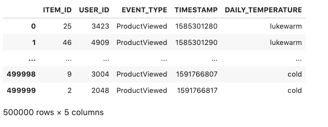
Context is environmental information that can shift rapidly over time, influencing your customer’s perception and behavior. We use DAILY_TEMPERATURE as an optional categorical attribute in our interactions dataset as context information at inference time.
Now let’s look at the distribution of temperatures from the interactions generated during the period of 3 months starting on March 25, 2020.
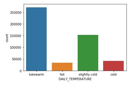
The preceding graphic shows that our interactions dataset doesn’t have many hot or cold days. This could be a good signal to the model to learn about the behavior customers display during those days and use that information at inference time. We can provide Amazon Personalize the weather context when asking for recommendations, and explore how the recommendations are influenced by this contextual information.
items.csv
This fictitious dataset simulates a product catalog for a CPG company.
The items dataset stores metadata about your items. This dataset is optional when using Amazon Personalize; however, in this use case we need to include attributes category and size to test the recommendations behavior.
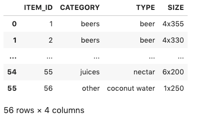
users.csv
This dataset is a subset of a fictitious dataset taken from the Retail Demo Store project.
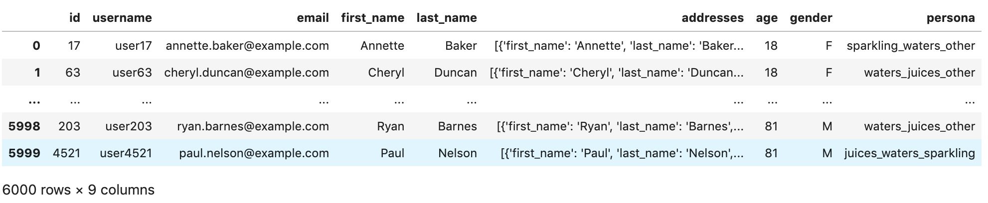
A users dataset stores metadata about your users. This can include information such as age, gender, name, and more. It’s an optional dataset when using Amazon Personalize.
For this post, we need the information from columns id and persona to be included in our model. persona is a categorical metadata field representing the categories of products that a customer likes and is used to test the recommendations behavior.
weather_data.csv
We use a real weather dataset provided by Weather Trends International to enrich the interactions dataset with temperature data.
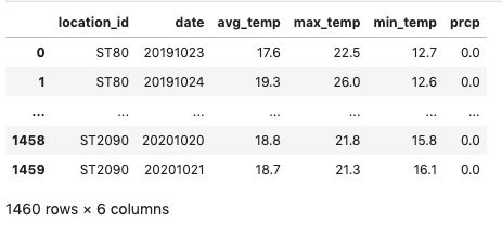
For simplicity, we keep only the rows representing Santiago de Chile, location_id = ‘ST650’.
Create Amazon Personalize components
When the datasets are ready to be imported, we’re ready to start creating an Amazon Personalize deployment. If you want to reproduce this process in your own account, you can use our sample notebook to complete the following steps:
- Create a dataset group with interactions, users, and items metadata datasets.
- Import historical data into each dataset.
- Configure a solution with a context-aware algorithm (aws-user-personalization) and train a solution version.
- Explore the solution version metrics.
- Create a campaign (managed recommendations endpoint).
- Query for personalized recommendations.
Explore Amazon Personalize recommendations
Now we can explore the recommendations provided by the campaign we created earlier. To do so, we pick a random user with ID 170 and get the top five beverages recommended for them with and without daily temperature as context.
The following screenshot shows the top five without context information.
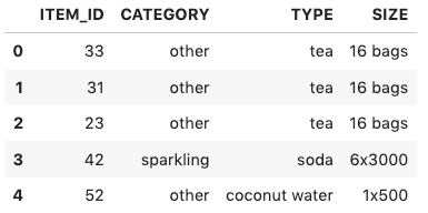
The following screenshot shows the top five with DAILY_TEMPERATURE = “cold”.

This user’s persona is other_waters_sparkling, which indicates a preference for those categories of beverages. The Amazon Personalize recommendations are consistent with their preferences with and without context. However, when we ask for recommendations on a cold day, the ranking of recommendations change:
- The category of the top three items in the ranking doesn’t change
- Tea item 33 went down from first to third in the ranking
- Coconut water, a refreshing item 52, was replaced by the same beverage in a bigger size format: item 15
These changes were driven by the behavior of customers in our dataset. For example, maybe user 170 likes different brands to prepare hot and iced tea, and the recommendations ranking is reflecting that preference on cold days.
Context is especially useful when dealing with new users without previous interactions. The following screenshot shows the top recommendations for a nonexistent user, ID 7000, without context.
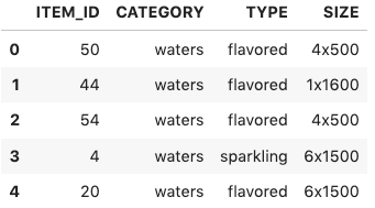
The following shows the recommendations for the same user with DAILY_TEMPERATURE = “hot”.
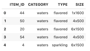
In the case of generating recommendations for a cold user, recommended items are the same, but the position in the ranking varies when considering a hot day vs. not providing context. In ecommerce with anonymous shopping functionality, this is particularly useful to prioritize which products to visualize, or suggest popular items to an unknown user considering their current context.
Conclusion
As stated in study How Context Affects Choice, context influences customer outcomes by altering the process by which decisions are made. Data like temperature, precipitation, device type, and channel of interaction can enrich models and improve the relevance of recommendations generated by Amazon Personalize. More relevant recommendations lead to better user experience and better business outcomes.
If you found this post useful and want to test how it works in real life, you can gather your own context data, or purchase datasets on AWS Data Exchange and use the approach of this post to put your use case into production. Feel free to explore any other creative ideas you can find.
If you want to recreate this use case with your own data, Daily Historical Weather Dataset – Demo is free for a month and code from this post is available on GitHub.
Additional resources about Amazon Personalize can be found on the Amazon Personalize GitHub repository.
About the Author
 Angel Goñi is an Enterprise Solutions Architect at AWS. He helps enterprise customers drive their digital transformation process leveraging AWS services. Usually works with Consumer Packaged Goods customers with emphasis on SAP migrations to AWS.
Build fast, sparse on-device models with the new TF MOT Pruning API

Posted by Yunlu Li and Artsiom Ablavatski
Introduction
Pruning is one of the core optimization techniques provided in the TensorFlow Model Optimization Toolkit (TF MOT). Not only does it help to significantly reduce model size, but it can also be used to accelerate CPU inference on mobile and web. With modern compute intensive models, the area of pruning as a model optimization technique has drawn significant attention, demonstrating that dense networks can be easily pruned (i.e. a fraction of the weights set to zero) with negligible quality degradation. Today, we are excited to announce a set of updates to TF MOT Pruning API that simplify pruning and enable developers to build sparse models for fast on-device inference.
Updates to TF MOT
TensorFlow has long standing support for neural network pruning via TensorFlow Model Optimization Toolkit (TF MOT) Pruning API. The API, featured in 2019, introduced essential primitives for pruning, and enabled researchers throughout the world with new optimization techniques. Today we are happy to announce experimental updates to the API that further advance model pruning. We are releasing tools that simplify the control of pruning and enable latency reduction for on-device inference.
The TF MOT Pruning API has extensive functionality that provides the user with tools for model manipulation:
prune_low_magnitudefunction appliesPruneLowMagnitudewrapper to every layer in the modelPruneLowMagnitudewrapper handles low-level pruning logicPruningSchedulecontrols when pruning is appliedPruningSummariescallback logs the pruning progress
These abstractions allow to control almost any aspect of model pruning (i.e. how to prune (PruneLowMagnitude), when to prune (PruningSchedule) and how to track the progress of the pruning (PruningSummaries) with the exception of what to prune, i.e. where PruneLowMagnitude wrapper is applied. We are happy to release an extension of TF MOT PruningPolicy, a class that controls which parts of the model the PruneLowMagnitude wrapper is applied to. The instance of PruningPolicy is used as an argument in the prune_low_magnitude function and provides the following functionalities:
- Controls where the pruning wrapper should be applied on per-layer basis through the
allow_pruningfunction - Checks that the whole model supports pruning via
ensure_model_supports_pruningfunction
PruningPolicy is an abstract interface, and it can have many implementations depending on the particular application. For latency improvements on CPU via XNNPACK, the concrete implementation PruneForLatencyOnXNNPack applies the pruning wrapper only to the parts of the model that can be accelerated via sparse on-device inference while leaving the rest of the network untouched. Such selective pruning allows an application to maintain model quality while targeting parts of the model that can be accelerated by sparsity.
The below example showcases the PruneForLatencyOnXNNPack policy in action on
MobileNetV2 (the full example is available in a recently introduced colab):
import tensorflow as tf
import tensorflow_model_optimization as tfmot
prune_low_magnitude = tfmot.sparsity.keras.prune_low_magnitude

# See the implementation of the function below.
model = load_model_for_pruning()

model_for_pruning = prune_low_magnitude(
    model, pruning_policy=tfmot.sparsity.keras.PruneForLatencyOnXNNPack())
In order to comply with the constraints of XNNPACK sparse inference the Keras implementation of MobileNetV2 model requires slight modification of the padding for the first convolution operation:
def load_model_for_pruning():
  input_tensor = tf.keras.layers.Input((224, 224, 3))
  input_tensor = tf.keras.layers.ZeroPadding2D(1)(input_tensor)
  model = tf.keras.applications.MobileNetV2(input_tensor=input_tensor)

  def clone_fn(layer):
    if layer.name == 'Conv1':
      # The default padding `SAME` for the first convolution is incompatible
      # with XNNPACK sparse inference.
      layer.padding = 'valid'
      # We ask the model to rebuild since we've changed the padding parameter.
      layer.built = False
    return layer

  return tf.keras.models.clone_model(model, clone_function=clone_fn)
The PruneForLatencyOnXNNPack policy applies the pruning wrapper only to convolutions with 1×1 kernel size since only these layers can be accelerated on CPU by as much as 2x using XNNPACK. The rest of the layers are left untouched allowing the network to recover after quality degradation at the pruning step. Also, the policy verifies that the model is amenable to being pruned by using the ensure_model_supports_pruning method. Once the sparse model has been trained and converted, we recommend using the TensorFlow Lite benchmark utility in debug mode to confirm that the final model is compatible with XNNPack’s sparse inference backend.
We hope that this newly introduced experimental API will be useful in practice and we will continue to improve its stability and flexibility in the future.
Compression and Latency Improvements
Model compression is another major benefit of applying pruning to a model. Using a smart compression format allows efficient storage of model weights which leads to a significant size reduction.
TFLite adopted the TACO format to encode sparse tensors. Compared to widely used formats like CSR and CSC, the TACO format has several advantages:
- It supports flexible traversal order to store a tensor in row-major or column-major formats easily.
- It supports multi-dimensional sparse tensors like the 4-D filter of a convolution op.
- It can represent block structure as the inner dimension of the tensor (example of a 4×4 tensor with 2×2 inner block structure).
We also adapted the format to use flexible data types for the metadata storing the indices of non-zero elements. This reduces the storage overhead for small tensors, or tensors with compact data types like int8_t.
In order to realize size reductions in practice during the model conversion, the tf.lite.Optimize.EXPERIMENTAL_SPARSITY optimization needs to be applied. This optimization handles examining the model for sparse tensors and converting them to an efficient storage format. It also works seamlessly with quantization and you can combine them to achieve more aggressive model compresion. The full example of such a conversion is shown below:
# Remove the pruning wrappers from the model.
model = tfmot.sparsity.keras.strip_pruning(model)

converter = tf.lite.TFLiteConverter.from_keras_model(model)
# We apply float16 quantization together with sparsity optimization that
# compactly stores pruned weights.
converter.optimizations = [
    tf.lite.Optimize.EXPERIMENTAL_SPARSITY,  # Enables size reduction optimization.
    tf.lite.Optimize.DEFAULT  # Enables quantization at conversion.
]
converter.target_spec.supported_types = [tf.float16]
tflite_buffer = converter.convert()
After applying the tf.lite.Optimize.EXPERIMENTAL_SPARSITY optimization together with PruneForLatencyOnXNNPack pruning policy, a ~2x size reduction can be achieved as is demonstrated in Figure 1:
|
Figure 1. Ablation study of MobileNetV2 model size (float32 and float16 types) with different sparsity levels using PruneForLatencyOnXNNPack pruning policy. Only the 1×1 convolutional layers are pruned and the rest of the layers are left dense. |
In addition to size reduction, pruning can provide inference acceleration on CPU via XNNPACK. Using the PruneForLatencyOnXNNPack pruning policy, we’ve conducted an ablation study of CPU inference latency for a MobileNetV2 model on Pixel 4 using TensorFlow Lite benchmark with the use_xnnpack option enabled:
 |
| Figure 2. Ablation study of CPU inference speed of MobileNetV2 model with different sparsity levels on a Pixel 4 device. |
This study in Figure 2 demonstrates 1.7x latency improvement when running on mobile devices using XNNPACK. The strategies for training the sparse MobileNetV2 model together with hyperparameters and pre-trained checkpoints are described in Elsen et al.
Pruning techniques & tips
Pruning aware training is a key step in model optimization. Many hyperparameters are involved in training and some of them like the pruning schedule and learning rate can have a dramatic impact on the final quality of the model. Though many strategies have been proposed, a simple yet effective 3-steps strategy (see Table 1) achieves strong performance for the majority of our use cases. The strategy builds on top of the well-proven approach from Zhu & Gupta and produces good results without extensive re-training:
|
Step |
Learning rate |
Duration |
Notes |
|
1. Pre-training or using pre-trained weights (optional) |
The same as for the regular dense network: starting from high value (possibly with warm-up) and ending with low value |
The same as for the regular dense network |
Paired with weight decay regularization this step helps the model to push unimportant weights towards 0 for pruning in the next step |
|
2. Iterative pruning |
Constant, mean of the learning rate values for the regular training |
30 to 100 epochs |
Iterative pruning step during which weights become sparse |
|
3. Fine-tuning |
The same as at the first stage but without warm up stage |
The same as at the first stage |
Helps to mitigate quality degradation after the pruning step |
3-step schedule for training the sparse model
The strategy inevitably leads to a substantial increase (~3x) in the training time. However, paired with the PolynomialDecay pruning schedule, this 3-step strategy achieves limited or no quality degradation with significantly pruned (>70%) neural networks.
Pruned models in MediaPipe
Together with the updates to the TF MOT Pruning API, we are happy to release pruned models for some of the MediaPipe solutions. The released models include pose and face detectors as well as a pruned hand tracking model. All of these models have been trained with the newly introduced functionality using the 3-steps pruning strategy. Compared with dense baselines the released pruned models have demonstrated significant model size reduction as well as superior performance when running on CPU via XNNPACK. Quality-wise the pruned models achieve similar metrics including in the evaluation on our fairness datasets (see model cards for details). Side-by-side demos of the solutions are shown below:

 |
| Figure 3. Comparison of dense (left) and sparse (right) models in the end-to-end examples of face (top) and pose (bottom) detection |
Pruning for GPU
While exploiting sparsity on GPUs can be challenging, recent work has made progress in improving the performance of sparse operations on these platforms. There is momentum for adding first-class support for sparse matrices and sparse operations in popular frameworks, and state-of-the-art GPUs have recently added hardware acceleration for some forms of structured sparsity. Going forward, improvements in software and hardware support for sparsity in both training and inference will be a key contributor to progress in the field.
Future directions
TF MOT offers a variety of model optimization methods, many of which have proven to be essential for efficient on-device model inference. We will continue to expand the TF MOT Pruning API with algorithms beyond low magnitude pruning, and also investigate the combination of pruning and quantization techniques to achieve even better results for on-device inference. Stay tuned!
Acknowledgments
Huge thanks to all who worked on this project: Karthik Raveendran, Ethan Kim, Marat Dukhan, Trevor Gale, Utku Evci, Erich Elsen, Frank Barchard, Yury Kartynnik, Valentin Bazarevsky, Matsvei Zhdanovich, Juhyun Lee, Chuo-Ling Chang, Ming Guang Yong, Jared Duke and Matthias Grundmann.
Why Nanneh Chehras is committed to being a mentor
The senior economist knows what it means to pursue a career path like hers, and she’s determined to help others along the way.Read More