Monthly Archives: July 2021

There are multiple scenarios in which you may want to use computer vision to detect small objects or symbols within a given image. Whether it’s detecting company logos on grocery store shelves to manage inventory, detecting informative symbols on documents, or evaluating survey or quiz documents that contain checkmarks or shaded circles, the size ratio of objects of interest to the overall image size is often very small. This presents a common challenge with machine learning (ML) models, because the processes performed by the models on an image can sometimes miss smaller objects when trying to reduce down and learn the details of larger objects in the image.

In this post, we demonstrate a preprocessing method to increase the size ratio of small objects with respect to an image and optimize the object detection capabilities of Amazon Rekognition Custom Labels, effectively solving the small object detection challenge.

Amazon Rekognition is a fully managed service that provides computer vision (CV) capabilities for analyzing images and video at scale, using deep learning technology without requiring ML expertise. Amazon Rekognition Custom Labels, an automated ML feature of Amazon Rekognition, lets you quickly train custom CV models specific to your business needs simply by bringing labeled images.

Solution overview

The preprocessing method that we implement is an image tiling technique. We discuss how this works in detail in a later section. To demonstrate the performance boost our preprocessing method presents, we train two Amazon Rekognition Custom Labels models—one baseline model and one tiling model—evaluate them on the same test dataset, and compare model results.

Data

For this post, we created a sample dataset to replicate many use cases containing small objects that have significant meaning or value within the document. In the following sample document, we’re interested in four object classes: empty triangles, solid triangles, up arrows, and down arrows. In the creation of this dataset, we converted each page of the PDF document into an image. The four object classes listed were labeled using Amazon SageMaker Ground Truth.

Baseline model

After you have a labeled dataset, you’re ready to train your Amazon Rekognition Custom Labels model. First we train our baseline model that doesn’t include the preprocessing technique. The first step is to set up our Amazon Rekognition Custom Labels project.

1. On the Amazon Rekognition console, choose Use Custom Labels.
2. Under Datasets, choose Create new dataset.
3. For Dataset name¸ enter cl-blog-original-train.

We repeat this process to create our Amazon SageMaker Ground Truth labeled test set called cl-blog-original-test.

3. Under Projects, choose Create new project.
4. For Project name, enter cl-blog-original.

5. On the cl-blog-original project details page, choose Train new model.
6. Reference the train and test set you created that Amazon Rekognition uses to train and evaluate the model.

The training time varies based on the size and complexity of the dataset. For reference, our model took about 1.5 hours to train.

After the model is trained, Amazon Rekognition outputs various metrics to the model dashboard so you can analyze the performance of your model. The main metric we’re interested in for this example is the F1 score, but precision and recall are also provided. F1 score measures a models’ overall accuracy, which is calculated as the mean of precision and recall. Precision measures how many model predictions are objects of interest, and recall measures how many objects of interest the model accurately predicted.

Our baseline model yielded an F1 score of about 0.40. The following results show that the model performs fairly well with regard to precision for the different labels, but fails to recall the labels across the board. The recall scores for down_arrow, empty_triangle, solid_triangle, and up_arrow are 0.27, 0.33, 0.33, and 0.17, respectively. Because precision and recall both contribute to the F1 score, the high precision scores for each label are brought down by the poor recall scores.

To improve our model performance, we explore a tiling approach in the next section.

Tiling approach model

Now that we’ve trained our baseline model and analyzed its performance, let’s see if tiling our original images into smaller images results in a performance increase. The idea here is that tiling our image into smaller images allows for the small symbol to appear with a greater size ratio when compared to the same small symbol in the original image. The first step before creating a labeled dataset in Ground Truth is to tile the images in our original dataset into smaller images. We then generate our labeled dataset with Ground Truth using this new tiled dataset, and train a new Amazon Rekognition Custom Labels tiled model.

1. Open up your preferred IDE and create two directories:
   1. original_images for storing the original document images
   2. tiled_images for storing the resulting tiled images
2. Upload your original images into the original_images directory.

For this post, we use Python and import a package called image_slicer. This package includes functions to slice our original images into a specified number of tiles and save the resulting tiled images into a specified folder.

3. In the following code, we iterate over each image in our original image folder, slice the image into quarters, and save the resulting tiled images into our tiled images folder.

import os
import image_slicer

for img in os.listdir("original_images"):
tiles = image_slicer.slice(os.path.join("original_images", img), 4, save=False)
image_slicer.save_tiles(
tiles, directory="tiled_images",
prefix=str(img).split(".")[0], format="png")

You can experiment with the number of tiles, because smaller symbols in more complex images may need a higher number of tiles, but four worked well for our set of images.

The following image shows an example output from the tiling script.

After our image dataset is tiled, we can repeat the same steps from training our baseline model.

4. Create a labeled Ground Truth cl-blog-tiled-train and cl-blog-tiled-test set.

We make sure to use the same images in our baseline-model-test set as our tiled-model-test set to ensure we’re maintaining an unbiased evaluation when comparing both models.

5. On the Amazon Rekognition console, on the cl-blog-tiled project details page, choose Train new model.
6. Reference the tiled train and test set you just created that Amazon Rekognition uses to train and evaluate the model.

After the model is trained, Amazon Rekognition outputs various metrics to the model dashboard so you can analyze the performance of your model. Our model predicts with a F1 score of about 0.68. The following results show that the recall improved for all labels at the expense of the precision of down_arrow and up_arrow. However, the improved recall scores were enough to boost our F1 score.

Results

When we compare the results of both the baseline model and the tiled model, we can observe that the tiling approach gave the new model a significant 0.28 boost in F1 score, from 0.40 to 0.68. Because the F1 score measures model accuracy, this means that the tiled model is 28% more likely to accurately identify small objects on a page than the baseline model. Although the precision for the down_arrow label dropped from 0.89 to 0.28 and the precision for the up_arrow label dropped from 0.71 to 0.68, the recall for all the labels significantly increased.

Conclusion

In this post, we demonstrated how to use tiling as a preprocessing technique to maximize the performance of Amazon Rekognition Custom Labels when detecting small objects. This method is a quick addition to improve the predictive accuracy of a Amazon Rekognition Custom Labels model by increasing the size ratio of small objects relative to the overall image.

For more information about using custom labels, see What Is Amazon Rekognition Custom Labels?

About the Authors

Alexa Giftopoulos is a Machine Learning Consultant at AWS with the National Security Professional Services team, where she develops AI/ML solutions for various business problems.

Sarvesh Bhagat is a Cloud Consultant for AWS Professional Services based out of Virginia. He works with public sector customers to help solve their AI/ML-focused business problems.

Akash Patwal is a Machine Learning Consultant at AWS where he builds AI/ML solutions for customers.

Read More

The world we live in is constantly changing, and so is the data that is collected to build models. One of the problems that is often seen in production environments is that the deployed model doesn’t behave the same way as it did during the training phase. This concept is generally called data drift or dataset shift, and can be caused by many factors, such as bias in sampling data that affects features or label data, the non-stationary nature of time series data, or changes in the data pipeline. Because machine learning (ML) models aren’t deterministic, it’s important to minimize the variance in the production environment by periodically monitoring the deployment environment for model drift and sending alerts and, if necessary, triggering retraining of the models with new data.

Amazon SageMaker is a fully managed service that enables developers and data scientists to quickly and easily build, train, and deploy ML models at any scale. After you train an ML model, you can deploy it on SageMaker endpoints that are fully managed and can serve inferences in real time with low latency. After you deploy your model, you can use Amazon SageMaker Model Monitor to continuously monitor the quality of your ML model in real time. You can also configure alerts to notify and trigger actions if any drift in model performance is observed. Early and proactive detection of these deviations enables you to take corrective actions, such as collecting new ground truth training data, retraining models, and auditing upstream systems, without having to manually monitor models or build additional tooling.

In this post, we present some techniques to detect covariate drift (one of the types of data drift) and demonstrate how to incorporate your own drift detection algorithms and visualizations with Model Monitor.

Types of data drift

Data drift can be classified into three categories depending on whether the distribution shift is happening on the input or on the output side, or whether the relationship between the input and the output has changed.

Covariate shift

In a covariate shift, the distribution of inputs changes over time, but the conditional distribution P(y|x) doesn’t change. This type of drift is called covariate shift because the problem arises due to a shift in the distribution of the covariates (features). For example, the training dataset for a face recognition algorithm may contain predominantly younger faces, while the real world may have a much larger proportion of older people.

Label shift

While covariate shift focuses on changes in the feature distribution, label shift focuses on changes in the distribution of the class variable. This type of shifting is essentially the reverse of covariate shift. An intuitive way to think about it might be to consider an unbalanced dataset; for example, if the spam to non-spam ratio of emails in our training set is 50%, but in reality, 10% of our emails are non-spam, then the target label distribution has shifted.

Concept shift

Concept shift is different from covariate and label shift in that it’s not related to the data distribution or the class distribution, but instead is related to the relationship between the two variables. For example, in stock analysis, the relationship between prior stock market data and the stock price is non-stationary. The relationship between the input data and the target variable changes over time, and the model needs to be refreshed often.

Now that we know the types of distribution shifts, let’s see how Model Monitor helps us in detecting data drifts. In the next section, we walk through setting up Model Monitor and incorporating our custom drift detection algorithms.

Model Monitor

Model Monitor offers four different types of monitoring capabilities to detect and mitigate model drift in real time:

• Data quality – Helps detect change in data schemas and statistical properties of independent variables and alerts when a drift is detected.
• Model quality – For monitoring model performance characteristics such as accuracy or precision in real time, Model Monitor allows you to ingest the ground truth labels collected from your applications. Model Monitor automatically merges the ground truth information with prediction data to compute the model performance metrics.
• Model bias –Model Monitor is integrated with Amazon SageMaker Clarify to improve visibility into potential bias. Although your initial data or model may not be biased, changes in the world may cause bias to develop over time in a model that has already been trained.
• Model explainability – Drift detection alerts you when a change occurs in the relative importance of feature attributions.

Deequ, which measures data quality, powers some of the Model Monitor pre-built monitors. You don’t require coding to utilize these pre-built monitoring capabilities. You also have the flexibility to monitor models by coding to provide custom analysis. All metrics emitted by Model Monitor can be collected and viewed in Amazon SageMaker Studio, so you can visually analyze your model performance without writing additional code.

In certain scenarios, the pre-built monitors may not be sufficient to generate sophisticated metrics to detect drifts, and may necessitate bringing your own metrics. In the next sections, we describe the setup to bring in your metrics by building a custom container.

Environment setup

For this post, we use a SageMaker notebook to set up Model Monitor and also visualize the drifts. We begin with setting up required roles and Amazon Simple Storage Service (Amazon S3) buckets to store our data:

region = boto3.Session().region_name

sm_client = boto3.client('sagemaker')

role = get_execution_role()
print(f"RoleArn: {role}")

# You can use a different bucket, but make sure the role you chose for this notebook
# has the s3:PutObject permissions. This is the bucket into which the data is captured
bucket = session.Session(boto3.Session()).default_bucket()
print(f"Demo Bucket: {bucket}")
prefix = 'sagemaker/DEMO-ModelMonitor'

s3_capture_upload_path = f's3://{bucket}/{prefix}/datacapture'
s3_report_path = f's3://{bucket}/{prefix}/reports'

Upload train dataset, test dataset, and model file to Amazon S3

Next, we upload our training and test datasets, and also the training model we use for inference. For this post, we use the Census Income Dataset from UCI Machine Learning Repository. The dataset consists of people’s income and several attributes that describe population demographics. The task is to predict if a person makes above or below $50,000. This dataset contains both categorical and integral attributes, and has several missing values. This makes it a good example to demonstrate model drift and detection.

We use XGBoost algorithm to train the model offline using SageMaker. We provide the model file for deployment. The training dataset is used for comparing with inference data to generate drift scores, while test dataset is used for computing how much the accuracy of the model has degraded due to drift. We provide more intuition on these algorithms in later steps.

The following code uploads our datasets and model to Amazon S3:

model_file = open("model/model.tar.gz", 'rb')
train_file = open("data/train.csv", 'rb')
test_file = open("data/test.csv", 'rb')

s3_model_key = os.path.join(prefix, 'model.tar.gz')
s3_train_key = os.path.join(prefix, 'train.csv')
s3_test_key = os.path.join(prefix, 'test.csv')

boto3.Session().resource('s3').Bucket(bucket).Object(s3_model_key).upload_fileobj(model_file)
boto3.Session().resource('s3').Bucket(bucket).Object(s3_train_key).upload_fileobj(train_file)
boto3.Session().resource('s3').Bucket(bucket).Object(s3_test_key).upload_fileobj(test_file)

Set up a Docker container

Model Monitor supports bringing your own custom model monitor containers. When you create a MonitoringSchedule, Model Monitor starts processing jobs for evaluating incoming inference data. While invoking the containers, Model Monitor sets up additional environment variables for you so that your container has enough context to process the data for that particular run of the scheduled monitoring. For the container code variables, see Container Contract Inputs. Of the available input environmental variables, we’re interested in dataset_source, output_path, and end_time:

"Environment": {
    "dataset_source": "/opt/ml/processing/endpointdata",
    "output_path": "/opt/ml/processing/resultdata",
    "end_time": "2019-12-01T16: 20: 00Z"
}

The dataset_source variable specifies the data capture location on the container, and end_time refers to the time of the last event capture. The custom drift algorithm is included in the src directory. For details on the algorithms, see the GitHub repo.

Now we build the Docker container and push it to Amazon ECR. See the following Dockerfile:

FROM python:3.8-slim-buster

RUN pip3 install pandas==1.1.4 numpy==1.19.4 scikit-learn==0.23.2 pyarrow==2.0.0 scipy==1.5.4 boto3==1.17.12

WORKDIR /home
COPY src/* /home/

ENTRYPOINT ["python3", "drift_detector.py"]

We build and push it to Amazon ECR with the following code:

from docker_utils import build_and_push_docker_image

repository_short_name = 'custom-model-monitor'

image_name = build_and_push_docker_image(repository_short_name)

Set up an endpoint and enable data capture

As we mentioned before, our model was trained using XGBoost, so we use XGBoostModel from the SageMaker SDK to deploy the model. Because we have a custom input parser, which includes imputation and one-hot encoding, we provide the inference entry point along with source directory, which includes the Scikit ColumnTransfomer model. The following code is the customer inference function:

script_path = pathlib.Path(__file__).parent.absolute()
with open(f'{script_path}/preprocess.pkl', 'rb') as f:
    preprocess = pickle.load(f) 


def input_fn(request_body, content_type):
    """
    The SageMaker XGBoost model server receives the request data body and the content type,
    and invokes the `input_fn`.

    Return a DMatrix (an object that can be passed to predict_fn).
    """

    if content_type == 'text/csv':        
        df = pd.read_csv(StringIO(request_body), header=None)
        X = preprocess.transform(df)
        
        X_csv = StringIO()
        pd.DataFrame(X).to_csv(X_csv, header=False, index=False)
        req_transformed = X_csv.getvalue().replace('n', '')
        
        return xgb_encoders.csv_to_dmatrix(req_transformed)
    else:
        raise ValueError(
            f'Content type {request_content_type} is not supported.'
        )

We also include the configuration for data capture, specifying the S3 destination, and sampling percentage with the endpoint deployment (see the following code). Ideally, we want to capture 100% of the incoming data for drift detection, but for a high traffic endpoint, we suggest reducing the sampling percentage so that the endpoint availability isn’t affected. Besides, Model Monitor might automatically reduce the sampling percentage if it senses the endpoint availability is affected.

from sagemaker.xgboost.model import XGBoostModel
from sagemaker.serializers import CSVSerializer
from sagemaker.model_monitor import DataCaptureConfig

model_url = f's3://{bucket}/{s3_model_key}'

xgb_inference_model = XGBoostModel(
    model_data=model_url,
    role=role,
    entry_point='inference.py',
    source_dir='script',
    framework_version='1.2-1',
)

data_capture_config = DataCaptureConfig(
                        enable_capture=True,
                        sampling_percentage=100,
                        destination_s3_uri=s3_capture_upload_path)

predictor = xgb_inference_model.deploy(
    initial_instance_count=1,
    instance_type='ml.c5.xlarge',
    serializer=CSVSerializer(),
    data_capture_config=data_capture_config)

After we deploy the model, we can set up a monitor schedule.

Create a monitor schedule

Typically, we create a processing job to generate baseline metrics of our training set. Then we create a monitor schedule to start periodic jobs to analyze incoming inference requests and generate metrics similar to baseline metrics. The inference metrics are compared with baseline metrics and a detailed report on constraints violation and drift in data quality is generated. Using SageMaker SDK simplifies the creation of baseline metrics and scheduling model monitor.

For the algorithms we use in this post (such as Wasserstein distance and Kolmogorov–Smirnov test), the container that we build needs access to both the training dataset and the inference data for computing metrics. This non-typical setup requires some low-level setup of the monitor schedule. The following code is the Boto3 request to set up the monitor schedule. The key fields are related to the container image URL and arguments to the container. We cover building containers in the next section. For now, note that we pass the S3 URL for training the dataset:

s3_train_path = f's3://{bucket}/{s3_train_key}'
s3_test_path = f's3://{bucket}/{s3_test_key}'
s3_result_path = f's3://{bucket}/{prefix}/result/{predictor.endpoint_name}'

sm_client.create_monitoring_schedule(
    MonitoringScheduleName=predictor.endpoint_name,
    MonitoringScheduleConfig={
        'ScheduleConfig': {
            'ScheduleExpression': 'cron(0 * ? * * *)'
        },
        'MonitoringJobDefinition': {
            'MonitoringInputs': [
                {
                    'EndpointInput': {
                        'EndpointName': predictor.endpoint_name,
                        'LocalPath': '/opt/ml/processing/endpointdata'
                    }
                },
            ],
            'MonitoringOutputConfig': {
                'MonitoringOutputs': [
                    {
                        'S3Output': {
                            'S3Uri': s3_result_path,
                            'LocalPath': '/opt/ml/processing/resultdata',
                            'S3UploadMode': 'EndOfJob'
                        }
                    },
                ]
            },
            'MonitoringResources': {
                'ClusterConfig': {
                    'InstanceCount': 1,
                    'InstanceType': 'ml.c5.xlarge',
                    'VolumeSizeInGB': 10
                }
            },
            'MonitoringAppSpecification': {
                'ImageUri': image_name,
                'ContainerArguments': [
                    '--train_s3_uri',
                    s3_train_path,
                    '--test_s3_uri',
                    s3_test_path,
                    '--target_label',
                    'income'
                ]
            },
            'StoppingCondition': {
                'MaxRuntimeInSeconds': 600
            },
            'Environment': {
                'string': 'string'
            },
            'RoleArn': role
        }
    }
)

Generate requests for the endpoint

After we deploy the model, we send traffic at a constant rate to the endpoints. The following code launches a thread to generate the requests for about 10 hours. Make sure to stop the kernel if you want to stop the traffic. We let the traffic generator run for a few hours to collect enough samples to visualize drift. The plots automatically refresh whenever there is new data.

def invoke_endpoint(ep_name, file_name, runtime_client):
    pre_time = time()
    with open(file_name) as f:
        count = len(f.read().split('n')) - 2 # Remove EOF and header
    
    # Calculate time needed to sleep between inference calls if we need to have a constant rate of calls for 10 hours
    ten_hours_in_sec = 10*60*60
    sleep_time = ten_hours_in_sec/count
    
    with open(file_name, 'r') as f:
        next(f) # Skip header
        
        for ind, row in enumerate(f):   
            start_time = time()
            payload = row.rstrip('n')
            response = runtime_client(data=payload)
            
            # Print every 15 minutes (900 seconds)
            if (ind+1) % int(count/ten_hours_in_sec*900) == 0:
                print(f'Finished sending {ind+1} records.')
            
            # Sleep to ensure constant rate. Time spent for inference is subtracted
            sleep(max(sleep_time - (time() - start_time), 0))
                
    print("Done!")
    
print(f"Sending test traffic to the endpoint {predictor.endpoint_name}.nPlease wait...")

thread = Thread(target = invoke_endpoint, args=(predictor.endpoint, 'data/infer.csv', predictor.predict))
thread.start()

Visualize the data drift

We use the entire dataset for training and synthetically generate a new dataset for inference by modifying statistical properties of some of the attributes from the original dataset as described in our GitHub repo.

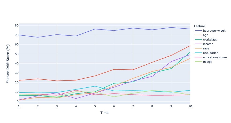
Normalized drift score per feature

A normalized drift score (in %) for each feature is computed by calculating the ratio of overlap of the distribution of incoming inference data with the original data to the original data. For categorical data, this is computed by summing the absolute of the difference in probability scores (training and inference) across each label. For numerical data, the training data is split into 10 bins (deciles), and the absolute of the difference in probability scores over bin is summed to calculate the drift score.

The following plot shows the drift scores over the time intervals. A few features have low to no drifts, while some features have drifts that are increasing over time, and finally hours-per-week has a large drift right from the start.

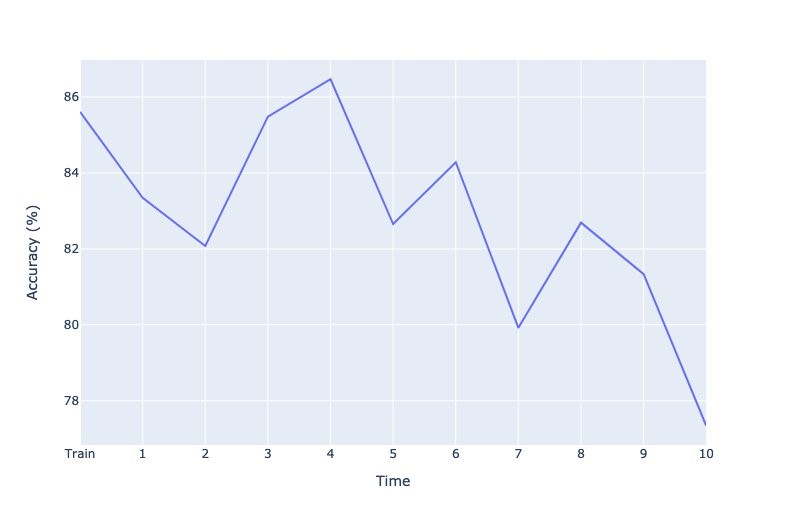
Projected drift in model accuracy

This metric provides a proxy of the accuracy of a model due to drift in inference data from the test data. The idea behind this approach is to determine how much percentage of the inference data is similar to the portion of the test data, where the model predicts well. For this metric, we use Isolation Forests to train one-class classifier, and generate scores for the portion of the test data that model predicted well, and for the inference data. The relative difference in the mean of these scores is the projected drift in accuracy.

The following plot shows the corresponding degradation in model accuracy due to drift in the incoming data. This demonstrates that covariate shift can reduce accuracy of a model. A few spikes in the metric can be attributed to the statistical nature of how the data is generated. This is only a proxy for model accuracy, and not the actual accuracy, which can only be known from the ground truth of the labels.

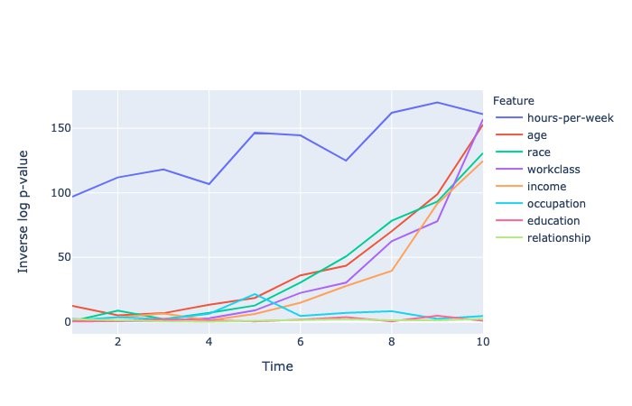
P-values of null test hypothesis

A null test hypothesis tests whether two samples (for this post, the training and inference datasets) are derived from the same general population. The p-value gives the probability of obtaining test results at least as extreme as the observations under the assumption that the null hypothesis is correct. A p-value threshold of 5% is used to decide whether the observed sample has drifted from the training data or not.

The following plot shows p-values of different attributes that have crossed the threshold at least once. The y-axis shows the inverse log of p-values to distinguish very small p-values. P-values for numerical attributes are obtained from Kolmogorov–Smirnov test, and for categorical attributes from Chi-square test.

Conclusion

Amazon SageMaker Model Monitor is a powerful tool to detect data drift. In this post, we showed how to easily integrate your custom data drift detection algorithms into Model Monitor, while benefiting from the heavy lifting that Model Monitor provides in terms of data capture and scheduling the monitor runs. The notebook provides a detailed step-by-step instruction on how to build a custom container and attach it to Model Monitor schedules. Give Model Monitor a try and leave your feedback in the comments.

About the Author

Vinay Hanumaiah is a Senior Deep Learning Architect at Amazon ML Solutions Lab, where he helps customers build AI and ML solutions to accelerate their business challenges. Prior to this, he contributed to the launch of AWS DeepLens and Amazon Personalize. In his spare time, he enjoys time with his family and is an avid rock climber.

Read More

With machine learning (ML), more powerful technologies have become available that can automate the task of detecting visual anomalies in a product. However, implementing such ML solutions is time-consuming and expensive because it involves managing and setting up complex infrastructure and having the right ML skills. Furthermore, ML applications need human oversight to ensure accuracy with anomaly detection, help provide continuous improvements, and retrain models with updated predictions. However, you’re often forced to choose between an ML-only or human-only system. Companies are looking for the best of both worlds, integrating ML systems into your workflow while keeping a human eye on the results to achieve higher precision.

In this post, we show how you can easily set up Amazon Lookout For Vision to train a visual anomaly detection model using a printed circuit board dataset, use a human-in-the-loop workflow to review the predictions using Amazon Augmented AI (Amazon A2I), augment the dataset to incorporate human input, and retrain the model.

Solution overview

Lookout for Vision is an ML service that helps spot product defects using computer vision to automate the quality inspection process in your manufacturing lines, with no ML expertise required. You can get started with as few as 30 product images (20 normal, 10 anomalous) to train your unique ML model. Lookout for Vision uses your unique ML model to analyze your product images in near-real time and detect product defects, allowing your plant personnel to diagnose and take corrective actions.

Amazon A2I is an ML service that makes it easy to build the workflows required for human review. Amazon A2I brings human review to all developers, removing the undifferentiated heavy lifting associated with building human review systems or managing large numbers of human reviewers, whether running on AWS or not.

To get started with Lookout for Vision, we create a project, create a dataset, train a model, and run inference on test images. After going through these steps, we show you how you can quickly set up a human review process using Amazon A2I and retrain your model with augmented or human reviewed datasets. We also provide an accompanying Jupyter notebook.

Architecture overview

The following diagram illustrates the solution architecture.

The solution has the following workflow:

1. Upload data from the source to Amazon Simple Storage Service (Amazon S3).
2. Run Lookout for Vision to process data from the Amazon S3 path.
3. Store inference results in Amazon S3 for downstream review.
4. Use Lookout for Vision to determine if an input image is damaged and validate that the confidence level is above 70%. If below 70%, we start a human loop for a worker to manually determine whether an image is damaged.
5. A private workforce investigates and validates the detected damages and provides feedback.
6. Update the training data with corresponding feedback for subsequent model retraining.
7. Repeat the retraining cycle for continuous model retraining.

Prerequisites

Before you get started, complete the following steps to set up the Jupyter notebook:

1. Create a notebook instance in Amazon SageMaker.
2. When the notebook is active, choose Open Jupyter.
3. On the Jupyter dashboard, choose New, and choose Terminal.
4. In the terminal, enter the following code:

cd SageMaker<br />git clone https://github.com/aws-samples/amazon-lookout-for-vision.git

5. Open the notebook for this post: Amazon-Lookout-for-Vision-and-Amazon-A2I-Integration.ipynb.

You’re now ready to run the notebook cells.

6. Run the setup environment step to set up the necessary Python SDKs and variables:

!pip install lookoutvision
!pip install simplejson

In the first step, you need to define the following:

• region – The Region where your project is located
• project_name – The name of your Lookout for Vision project
• bucket – The name of the Amazon S3 bucket where we output the model results
• model_version – Your model version (the default setting is 1)

# Set the AWS region
region = '<AWS REGION>'

# Set your project name here
project_name = '<CHANGE TO AMAZON LOOKOUT FOR VISION PROJECT NAME>'

# Provide the name of the S3 bucket where we will output results and store images
bucket = '<S3 BUCKET NAME>'

# This will default to a value of 1; Since we're training a new model, leave this set to a value of 1
model_version = '1'

7. Create the S3 buckets to store images:

!aws s3 mb s3://{bucket}

8. Create a manifest file from the dataset by running the cell in the section Create a manifest file from the dataset in the notebook.

Lookout for Vision uses this manifest file to determine the location of the files, as well as the labels associated with the files.

Upload circuit board images to Amazon S3

To train a Lookout for Vision model, we need to copy the sample dataset from our local Jupyter notebook over to Amazon S3:

# Upload images to S3 bucket:
!aws s3 cp circuitboard/train/normal s3://{bucket}/{project_name}/training/normal --recursive
!aws s3 cp circuitboard/train/anomaly s3://{bucket}/{project_name}/training/anomaly --recursive

!aws s3 cp circuitboard/test/normal s3://{bucket}/{project_name}/validation/normal --recursive
!aws s3 cp circuitboard/test/anomaly s3://{bucket}/{project_name}/validation/anomaly –recursive

Create a Lookout for Vision project

You have a couple of options on how to create your Lookout for Vision project: the Lookout for Vision console, the AWS Command Line Interface (AWS CLI), or the Boto3 SDK. We chose the Boto3 SDK in this example, but highly recommend you check out the console method as well.

The steps we take with the SDK are:

1. Create a project (the name was defined at the beginning) and tell your project where to find your training dataset. This is done via the manifest file for training.
2. Tell your project where to find your test dataset. This is done via the manifest file for test.

This second step is optional. In general, all test-related code is optional; Lookout for Vision also works with just a training dataset. We use both because training and testing is a common (best) practice when training AI and ML models.

Create a manifest file from the dataset

Lookout for Vision uses this manifest file to determine the location of the files, as well as the labels associated with the files. See the following code:

#Create the manifest file

from lookoutvision.manifest import Manifest
mft = Manifest(
    bucket=bucket,
    s3_path="{}/".format(project_name),
    datasets=["training", "validation"])
mft_resp = mft.push_manifests()
print(mft_resp)

Create a Lookout for Vision project

The following command creates a Lookout for Vision project:

# Create an Amazon Lookout for Vision Project

from lookoutvision.lookoutvision import LookoutForVision
l4v = LookoutForVision(project_name=project_name)
# If project does not exist: create it
p = l4v.create_project()
print(p)
print('Done!')

Create and train a model

In this section, we walk through the steps of creating the training and test datasets, training the model, and hosting the model.

Create the training and test datasets from images in Amazon S3

After we create the Lookout for Vision project, we create the project dataset by using the sample images we uploaded to Amazon S3 along with the manifest files. See the following code:

dsets = l4v.create_datasets(mft_resp, wait=True)
print(dsets)
print('Done!')

Train the model

After we create the Lookout for Vision project and the datasets, we can train our first model:

l4v.fit(
    output_bucket=bucket,
    model_prefix="mymodel_",
    wait=True)

When training is complete, we can view available model metrics:

met = Metrics(project_name=project_name)

met.describe_model(model_version=model_version)

You should see an output similar to the following.

Host the model

Before we can use our newly trained Lookout for Vision model, we need to host it:

l4v.deploy(
    model_version=model_version,
    wait=True)

Set up Amazon A2I to review predictions from Lookout for Vision

In this section, you set up a human review loop in Amazon A2I to review inferences that are below the confidence threshold. You must first create a private workforce and create a human task UI.

Create a workforce

You need to create a workforce via the SageMaker console. Note the ARN of the workforce and enter its value in the notebook cell:

WORKTEAM_ARN = 'your workforce team ARN'

The following screenshot shows the details of a private team named lfv-a2i and its corresponding ARN.

Create a human task UI

You now create a human task UI resource: a UI template in liquid HTML. This HTML page is rendered to the human workers whenever a human loop is required. For over 70 pre-built UIs, see the amazon-a2i-sample-task-uis GitHub repo.

Follow the steps provided in the notebook section Create a human task UI to create the web form, initialize Amazon A2I APIs, and inspect output:

...
def create_task_ui():
    '''
    Creates a Human Task UI resource.

    Returns:
    struct: HumanTaskUiArn
    '''
    response = sagemaker_client.create_human_task_ui(
        HumanTaskUiName=taskUIName,
        UiTemplate={'Content': template})
    return response
...

Create a human task workflow

Workflow definitions allow you to specify the following:

• The worker template or human task UI you created in the previous step.
• The workforce that your tasks are sent to. For this post, it’s the private workforce you created in the prerequisite steps.
• The instructions that your workforce receives.

This post uses the Create Flow Definition API to create a workflow definition. The results of human review are stored in an Amazon S3 bucket, which can be accessed by the client application. Run the cell Create a Human task Workflow in the notebook and inspect the output:

create_workflow_definition_response = sagemaker_client.create_flow_definition(
        FlowDefinitionName = flowDefinitionName,
        RoleArn = role,
        HumanLoopConfig = {
            "WorkteamArn": workteam_arn,
            "HumanTaskUiArn": humanTaskUiArn,
            "TaskCount": 1,
            "TaskDescription": "Select if the component is damaged or not.",
            "TaskTitle": "Verify if the component is damaged or not"
        },
        OutputConfig={
            "S3OutputPath" : a2i_results
        }
    )
flowDefinitionArn = create_workflow_definition_response['FlowDefinitionArn'] 
# let's save this ARN for future use

Make predictions and start a human loop based on the confidence level threshold

In this section, we loop through an array of new images and use the Lookout for Vision SDK to determine if our input images are damaged or not, and if they’re above or below a defined threshold. For this post, we set the threshold confidence level at .70. If our result is below .70, we start a human loop for a worker to manually determine if our image is normal or an anomaly. See the following code:

...

SCORE_THRESHOLD = .70

for fname in Incoming_Images_Array:
    #Lookout for Vision inference using detect_anomalies
    fname_full_path = (Incoming_Images_Dir + "/" + fname)
    with open(fname_full_path, "rb") as image:
        modelresponse = L4Vclient.detect_anomalies(
            ProjectName=project_name,
            ContentType="image/jpeg",  # or image/png for png format input image.
            Body=image.read(),
            ModelVersion=model_version,
            )
        modelresponseconfidence = (modelresponse["DetectAnomalyResult"]["Confidence"])

    if (modelresponseconfidence < SCORE_THRESHOLD):
...
        # start an a2i human review loop with an input
        start_loop_response = a2i.start_human_loop(
            HumanLoopName=humanLoopName,
            FlowDefinitionArn=flowDefinitionArn,
            HumanLoopInput={
                "InputContent": json.dumps(inputContent)
            }
        )
... 

You should get the output shown in the following screenshot.

Complete your review and check the human loop status

If inference results are below the defined threshold, a human loop is created. We can review the status of those jobs and wait for results:

...
completed_human_loops = []
for human_loop_name in human_loops_started:
    resp = a2i.describe_human_loop(HumanLoopName=human_loop_name)
    print(f'HumanLoop Name: {human_loop_name}')
    print(f'HumanLoop Status: {resp["HumanLoopStatus"]}')
    print(f'HumanLoop Output Destination: {resp["HumanLoopOutput"]}')
    print('n')
    
    if resp["HumanLoopStatus"] == "Completed":
        completed_human_loops.append(resp)
workteamName = workteam_arn[workteam_arn.rfind('/') + 1:]
print("Navigate to the private worker portal and do the tasks. Make sure you've invited yourself to your workteam!")
print('https://' + sagemaker_client.describe_workteam(WorkteamName=workteamName)['Workteam']['SubDomain'])

The work team sees the following screenshot to choose the correct label for the image.

View results of the Amazon A2I workflow and move objects to the correct folder for retraining

After the work team members have completed the human loop tasks, let’s use the results of the tasks to sort our images into the correct folders for training a new model. See the following code:

...

    # move the image to the appropriate training folder
    if (labelanswer == "Normal"):
        # move object to the Normal training folder s3://a2i-lfv-output/image_folder/normal/
        !aws s3 cp {taskObjectResponse} s3://{bucket}/{project_name}/train/normal/
    else:
        # move object to the Anomaly training folder
        !aws s3 cp {taskObjectResponse} s3://{bucket}/{project_name}/train/anomaly/
...

Retrain your model based on augmented datasets from Amazon A2I

Training a new model version can be triggered as a batch job on a schedule, manually as needed, based on how many new images have been added to the training folders, and so on. For this example, we use the Lookout for Vision SDK to retrain our model using the images that we’ve now included in our modified dataset. Follow the accompanying Jupyter notebook downloadable from [GitHub-LINK] for the complete notebook.

# Train the model!
l4v.fit(
    output_bucket=bucket,
    model_prefix="mymodelprefix_",
    wait=True)

You should see an output similar to the following.

Now that we’ve trained a new model using newly added images, let’s check the model metrics! We show the results from the first model and the second model at the same time:

# All models of the same project
met.describe_models()

You should see an output similar to the following. The table shows two models: a hosted model (ModelVersion:1) and the retrained model (ModelVersion:2). The performance of the retrained model is better with the human reviewed and labeled images.

Clean up

Run the Stop the model and cleanup resources cell to clean up the resources that were created. Delete any Lookout for Vision projects you’re no longer using, and remove objects from Amazon S3 to save costs. See the following code:

#If you are not using the model, stop to save costs! This can take up to 5 minutes.

#change the model version to whichever model you're using within your current project
model_version='1'
l4v.stop_model(model_version=model_version)

Conclusion

This post demonstrated how you can use Lookout for Vision and Amazon A2I to train models to detect defects in objects unique to your business and define conditions to send the predictions to a human workflow with labelers to review and update the results. You can use the human labeled output to augment the training dataset for retraining to improve the model accuracy.

Start your journey towards industrial anomaly detection and identification by visiting the Lookout for Vision Developer Guide and the Amazon A2I Developer Guide.

About the Author

Dennis Thurmon is a Solutions Architect at AWS, with a passion for Artificial Intelligence and Machine Learning. Based in Seattle, Washington, Dennis worked as a Systems Development Engineer on the Amazon Go and Amazon Books team before focusing on helping AWS customers bring their workloads to life in the AWS Cloud.

Amit Gupta is an AI Services Solutions Architect at AWS. He is passionate about enabling customers with well-architected machine learning solutions at scale.

Neel Sendas is a Senior Technical Account Manager at Amazon Web Services. Neel works with enterprise customers to design, deploy, and scale cloud applications to achieve their business goals. He has worked on various ML use cases, ranging from anomaly detection to predictive product quality for manufacturing and logistics optimization. When he is not helping customers, he dabbles in golf and salsa dancing.

Read More