Which Mutual Information Representation Learning Objectives are Sufficient for Control?

Processing raw sensory inputs is crucial for applying deep RL algorithms to real-world problems.
For example, autonomous vehicles must make decisions about how to drive safely given information flowing from cameras, radar, and microphones about the conditions of the road, traffic signals, and other cars and pedestrians.
However, direct “end-to-end” RL that maps sensor data to actions (Figure 1, left) can be very difficult because the inputs are high-dimensional, noisy, and contain redundant information.
Instead, the challenge is often broken down into two problems (Figure 1, right): (1) extract a representation of the sensory inputs that retains only the relevant information, and (2) perform RL with these representations of the inputs as the system state.


Figure 1. Representation learning can extract compact representations of states for RL.

A wide variety of algorithms have been proposed to learn lossy state representations in an unsupervised fashion (see this recent tutorial for an overview).
Recently, contrastive learning methods have proven effective on RL benchmarks such as Atari and DMControl (Oord et al. 2018, Stooke et al. 2020, Schwarzer et al. 2021), as well as for real-world robotic learning (Zhan et al.).
While we could ask which objectives are better in which circumstances, there is an even more basic question at hand: are the representations learned via these methods guaranteed to be sufficient for control?
In other words, do they suffice to learn the optimal policy, or might they discard some important information, making it impossible to solve the control problem?
For example, in the self-driving car scenario, if the representation discards the state of stoplights, the vehicle would be unable to drive safely.
Surprisingly, we find that some widely used objectives are not sufficient, and in fact do discard information that may be needed for downstream tasks.

Safety Envelopes using Light Curtains with Probabilistic Guarantees

Fig. 1: The safety envelope (in green) is an imaginary surface that separates the robot from all obstacles in its environment. As long as the robot never intersects the safety envelope, it is guaranteed to not collide with any obstacle. Our task is to estimate this envelope.

Safe navigation and obstacle detection

Consider the scene in Fig. 1 that a mobile robot wishes to navigate safely. The scene contains many obstacles such as walls, poles, and walking people. Obstacles could be arbitrarily distributed, their motion might be haphazard, and they may enter and leave the environment in an undetermined manner. This situation is commonly encountered in a variety of robotics tasks such as indoor and outdoor robot navigation, autonomous driving, and robot delivery. The robot must accurately and reliably detect all obstacles (static and dynamic) in the scene to avoid colliding with them and navigate safely. Therefore, it must estimate the safety envelope of the scene.

What is a safety envelope?

We define the safety envelope as an imaginary surface that separates the robot from all obstacles in its environment. As long as the robot never intersects the safety envelope, it is guaranteed to not collide with any obstacles! How can the robot accurately estimate the location of the safety envelope? Can it provide any guarantees about its ability to discover obstacles? In our recent paper published at RSS 2021, we answer these questions in the affirmative using a novel sensor called programmable light curtains.

What are light curtains?

Fig. 2: Comparing a standard LiDAR sensor and a programmable light curtain. A LiDAR detects points in the entire scene but sparsely. A light curtain detects points that intersect a user-specified surface at a much higher resolution.

A programmable light curtain is a 3D sensor recently invented at CMU. It can measure the depth of any user-specified 2D vertical surface (“curtain”) in the environment. A common strategy for 3D sensing is to use LiDARs. LiDARs have become ubiquitous in robotics and autonomous driving. However, they can be low resolution, expensive and slow. In contrast, light curtains are relatively inexpensive, faster, and of much higher resolution!

LiDAR (Velodyne) Light curtain
Low resolution (128 rows) High resolution (1280 rows)
Expensive (~$100,000) Inexpensive (~$1,000)
Slow (5-20 Hz) Fast (60 Hz)
No control required User control required

Most importantly, light curtains are a controllable sensor: the user selects a vertical 2D surface, and the light curtain detects objects intersecting that surface. This is a fundamentally different sensing paradigm from LiDARs. LiDARs passively sense the entire scene without any user input. However, light curtains can be actively controlled by the user to focus their sensing capacity on specific regions of interest. While controllability is clearly a desirable feature, it also presents a unique challenge: light curtains require the user to select which locations to sense. How should we place light curtains to accurately estimate the safety envelope of a scene?

Random curtains can reliably discover obstacles

Fig. 3: A heist scene from the movie Ocean’s Twelve. The robber needs to try extremely hard to avoid intersecting the randomly moving lasers. The same principle applies to randomly placed light curtains: they detect (sufficiently large) obstacles with very high probability. It is virtually impossible to evade random curtains!

Suppose we have a scene with no prior knowledge of where the obstacles are. How should we place light curtains to discover them? Surprisingly, we answered this question by taking inspiration from heist films such as Ocean’s Twelve. In a scene from this movie shown in Fig. 3, the robber attempts to evade a museum’s security system consisting of randomly moving laser detectors. The robber needs to try extremely hard, literally bending over backward, to avoid intersecting the lasers. Although the robber managed to pull it off in the movie, it is clear that this would be virtually impossible in the real world.

Fig. 4: Examples of random light curtains (in blue). The points on the obstacles that are intersected and detected by random curtains are shown in green. Random curtains are able to detect obstacles with high probability.

Light curtains are nothing but moving laser detectors! Therefore, our insight is to place curtains at random locations in the scene. We refer to them as “random curtains”, as shown in Fig. 4. It turns out to be incredibly hard for (sufficiently large) obstacles to avoid getting detected by random curtains. We place random curtains to quickly discover unknown objects and estimate the safety envelope of the scene.

In the section on theoretical analysis of random curtains near the end of this blog post, we will present a novel analytical technique that actually computes the probability of random curtains intersecting and detecting obstacles. The analytical probabilities act as safety guarantees for our perception system towards detecting and avoiding obstacles.

Forecasting safety envelopes

Fig. 5 We wish to estimate the safety envelope of a dynamic scene across time. Once the envelope is estimated in the current timestep, we use a machine learning-based forecasting model to predict the change in the location of the safety envelope. This allows us to efficiently track the safety envelope.

Assume that we have already estimated the safety envelope in the current timestep. As objects move and the scene changes with time, we wish to estimate the safety envelope for the next timestep. In this case, it may be inefficient to explore the scene from scratch by randomly placing curtains. Instead, we use machine learning to train a neural network to forecast how the safety envelope will evolve in the next timestep. The inputs to the network are all light curtain measurements from previous timesteps. The output is the predicted change in the envelope’s position in the next timestep. We use DAgger [Ross et. al. 2011], a standard imitation learning algorithm, to train such a forecasting model from data. By predicting how the safety envelope will move, we can directly sense the locations where obstacles are anticipated to be and efficiently track the safety envelope.

Active light curtain placement pipeline

Fig. 6: Our pipeline for estimating the safety envelope of a dynamic scene. It combines two components: a machine learning-based forecasting model to predict how the envelope will move, and random curtain placements to discover obstacles and update the predictions. Light curtains are also placed to sense the predicted location of the envelope.

Our overall pipeline for placing light curtains to estimate and track the safety envelope is as follows. Given previous light curtain measurements, we train a neural network to forecast how the safety envelope of the scene will evolve in the next timestep. We then place light curtains to sense the predicted locations. At the same time, we place random light curtains to discover obstacles and update our predictions. Finally, the light curtain measurements are input back to the forecasting method, closing the loop.

Real-world results

Here is our method in action in the real world! The scene consists of multiple people walking in front of the light curtain device at various speeds and in different patterns. Our method, which combines learning-based forecasting and random curtain placement, tries to estimate the safety envelope of this dynamic scene at each timestep.

The middle video shows the light curtain placed at the estimated location of the safety envelope in black. It also shows a LiDAR point cloud in red, used only for visualization purposes (our method only uses light curtain measurements). The video on the right shows intersection points, i.e. the points detected by the light curtain when it intersects object surfaces in green. These are aggregated across multiple frames to visualize the motion of obstacles.

Brisk Walking

Relaxed Walking

Many people (structured walking)

Many people (haphazard, occluded walking)

Fast motion

In all of the above videos, the light curtain is able to accurately estimate the safety envelope and produce a large number of intersection points. Due to the guarantees of high detection probability, our method generalizes to a varying number of obstacles (one vs. two vs. five people), a large range of motion (relaxed vs. brisk vs. extremely fast and sudden motion), and different patterns of motion (structured vs. complicated and haphazard).

Fig. 7: Quantitative analysis of safety envelope estimation, compared to various baselines.

Fig. 7 shows a quantitative analysis of our method compared to various baselines. We compute the Huber loss (related to thesmooth-L1 loss“) of the ratio between the predicted and true safety envelope location. We compare against a non-learning based handcrafted baseline. The baseline carefully alternates between moving the light curtain forward and backward, resulting in “hugging” the obstacles. We also compare against using only random curtains and using various neural network architectures. We include ablation experiments that remove one component of our method at a time (random curtains and forecasting) to demonstrate that both are crucial to our performance. Our method outperforms all baselines. Please see our paper for more experiments and evaluation metrics.

Theoretical analysis of random curtain detection

Previously, we mentioned that random light curtains can detect obstacles with a high probability. Can we perform any theoretical analysis to actually compute this probability? Can we compute the probability of a random curtain detecting an obstacle of a given shape, size, and location? If so, these probabilities can act as safety guarantees that help certify the ability of our perception system to detect and avoid obstacles. Before we begin analyzing random curtains, we must first understand how they are generated.

Constraint Graph and generating random curtains

Fig. 8: The constraint graph from the top-down view. Nodes correspond to locations that can be imaged. Two nodes are connected by an edge if they can be imaged sequentially while satisfying the physical constraints of the light curtain device.

In order to generate any light curtain, we need to account for the physical constraints of the light curtain device. These are encoded into a constraint graph (see Fig. 8). The nodes of the graph represent locations where the light curtain might be placed. The nodes are organized into “camera rays” indexed by (t in {1, dots, T}) from left to right. A light curtain is created by imaging one node per ray, from left to right. An edge exists between two nodes if they can be imaged consecutively.

Fig. 9: Any path in the constraint graph represents a feasible light curtain. Random curtains can be generated by performing random walks in the graph.

What decides whether an edge exists between two nodes? The light curtain device contains a rotating mirror that redirects and shoots light into the scene. By specifying the angle of rotation, light can be beamed at the desired locations to be imaged. However, the mirror, being a physical device, has velocity and acceleration limits. Therefore, we add an edge between two nodes only if the mirror can rotate fast enough to image those two locations one after the other.

This means that any path in the constraint graph connecting the leftmost ray (t=1) to the rightmost ray (t=T) represents a feasible light curtain! Furthermore, random curtains can be generated by performing a random walk through the graph. The random walk is performed by starting from a node on the leftmost ray. In each iteration, a node on the next ray is randomly sampled among the neighbors of the current node from some probability distribution (e.g. uniform distribution). This process is repeated till the rightmost ray is reached. Fig. 9 shows examples of actual random curtains generated this way.

Computing detection probability using Dynamic Programming

Fig. 10 Given an obstacle (in blue and red), some random curtains detect the obstacle (in yellow) but some don’t. We wish to compute the probability of detection.

Assume that we are given the shape, size, and location of an obstacle (bluered shape in Fig. 10). Some random curtains will intersect and detect the obstacle (detections are shown in yellow), but other random curtains will miss the obstacle. Can we compute the probability of detection?

A naive approach would be to enumerate the set of all feasible light curtains and sum the probabilities of sampling those curtains that detect the object. Unfortunately, this is impractical because the number of feasible curtains is exponentially large! Another approach is to use Monte Carlo sampling for estimating the detection probability. In this method, we sample a large number of random curtains and output the fraction of the sampled curtains that detect the obstacle. While this approach is simple, we will show later that it requires a large number of samples to be drawn, and only produces stochastic estimates of the true probability.

Instead, we have developed an analytical and efficient approach to compute the detection probability, using dynamic programming. We first divide the overall problem into multiple sub-problems. Let us represent (mathbf{x}_t) to be a node on the (t)-th ray. Let us define (P_mathrm{det}(mathbf{x}_t)) to be the the probability that “sub-curtains” i.e. partial random curtains starting from node (mathbf{x}_t) and ending at a rightmost node will detect the obstacle. We wish to compute (P_mathrm{det}(cdot)) for every node in the constraint graph. Conveniently, these sub-problems satisfy a recursive relationship! If the obstacle is detected at node (mathbf{x}_t), (P_mathrm{det}(mathbf{x}_t)) is trivially equal to (1). If not, it is equal to the sum of detection probabilities of sub-curtains starting at (mathbf{x}_t)’s child nodes (mathbf{x}_{t+1}), weighted by the probability (P(mathbf{x}_t rightarrow mathbf{x}_{t+1})) of transitioning to (mathbf{x}_{t+1}). This is expressed by the equation below.

$$
P_mathrm{det}(mathbf{x}_{t}) =
begin{cases}
1 & text{if obstacle is detected at node } mathbf{x}_{t}\
sum_{mathbf{x}_{t+1}} P(mathbf{x}_{t} rightarrow mathbf{x}_{t+1})~P_mathrm{det}(mathbf{x}_{t+1}) & text{otherwise}
end{cases} tag{1}
$$

Fig. 11: Dynamic programming exploits the structure of the constraint graph to efficiently and analytically compute the overall detection probability. It recursively iterates over all nodes and edges in the graph only once, from right to left.

In order to apply dynamic programming, we start at nodes on the rightmost ray (T). (P_mathrm{det}(cdot)) for these nodes is simply (1) or (0), depending on whether the obstacle is detected at these locations or not. Then, we iterate over all nodes in the graph from right to left (see Fig. 11) and apply the recursive formula in Eqn. 1. Once we have the sub-curtain detection probabilities for the leftmost nodes, the overall detection probability is simply (sum_{mathbf{x}_1} P_mathrm{init}(mathbf{x}_1)~P_mathrm{det}(mathbf{x}_1)), where (P_mathrm{init}(mathbf{x}_1)) is the probability of sampling (mathbf{x}_1) as the starting node of the random curtain.

Note that our method computes the true detection probability precisely — there is no stochasticity or noise in the estimates. It is also very efficient: we only need to iterate over all nodes and edges in the graph once.

An example of random curtain analysis

Fig. 12: The probability of detecting an average-sized car and an average-sized pedestrian by random curtains, as a function of the time taken to place multiple random curtains. The detection probability increases exponentially as more random curtains are placed.

Let us look at an example of random curtain analysis in Fig. 12. The X-axis shows the time taken to place multiple random curtains at 60 Hz. The Y-axis shows the detection probability of an average-sized car and an average-sized pedestrian. Average sizes were computed from KITTI, a large-scale autonomous driving benchmark dataset. Let (p) be the probability of detecting an obstacle by a single random curtain. If (n) curtains are sampled independently and placed, the probability that at least one of them will detect the object is (1-(1-p)^n), which increases exponentially with (n). Thanks to the high speed of light curtains, within as low as 67 milliseconds, we are able to guarantee the detection of an average-sized pedestrian with more than 95% probability and an average-sized car with more than 99% probability!

Comparison to sampling-based estimation

Fig. 13: Comparing the speed and precision of estimating the random curtain detection probability using dynamic programming (our method) and Monte Carlo sampling.

In traditional Monte Carlo estimation, we sample a large number of random curtains by performing multiple forward passes through the constraint graph. Then, we output the fraction of the sampled curtains that detect the obstacle. This produces an unbiased estimate of the detection probability, with a variance that decreases with the number of samples used. Fig. 13 show the estimates produced by each method with 95% confidence intervals, versus their runtime (in log-scale). Monte Carlo (MC) sampling produces noisy estimate of the true probability whereas our dynamic programming (DP) approach produces precise estimates (zero uncertainty); such precise estimates are useful for reliably evaluating the safety and robustness of our perception system. Furthermore, DP is orders of magnitude faster (takes 0.8 seconds) than MC since MC requires a large number of samples to converge to our estimate.

We have created an interactive web-based demo of random curtain analysis! The user can draw any shape, size, and location of the obstacle. The demo runs dynamic programming to compute the random curtain detection probability and displays the analysis. The demo also generates random curtains and visualizes detections of the obstacle. Click on the link to check it out!

Conclusion

We presented a method to estimate the safety envelope of a scene: a hypothetical surface that separates the robot from all obstacles in the environment. We used programmable light curtains, an actively controllable, resource-efficient sensor to directly estimate the safety envelope. Using a dynamic programming-based approach, we showed that random light curtains can discover obstacles with high-probability guarantees. We combined this with a machine learning-based forecasting method to efficiently track the safety envelope. This enables our robot perception system to accurately estimate safety envelopes, while our probabilistic guarantees help certify its accuracy and safety. This work is a step towards safe robot navigation using inexpensive controllable sensors.

Further reading

If you’re interested in more details, please check out the links to the full paper, the project website, talk, demo, and more!

Citation

This blog post is based on the following paper :

Siddharth Ancha, Gaurav Pathak, Srinivasa Narasimhan, and David Held.
Active Safety Envelopes using Light Curtains with Probabilistic Guarantees.
In Proceedings of Robotics: Science and Systems (RSS), July 2021.

Acknowledgements

Thanks to David Held, Srinivasa Narasimhan and Paul Liang for feedback on this post!

This material is based upon work supported by the National Science Foundation under Grants No. IIS-1849154, IIS-1900821 and by the United States Air Force and DARPA under Contract No. FA8750-18-C-0092. All opinions, findings, and conclusions or recommendations expressed in this post are those of the author(s) and do not necessarily reflect the views of Carnegie Mellon University, National Science Foundation, United States Air Force and DARPA.

Read More

NVIDIA CEO Receives Semiconductor Industry’s Top Honor

By the time the night was over, it felt like Jensen Huang had given everyone in the ballroom a good laugh and a few things to think about.

The annual dinner of the Semiconductor Industry Association — a group of companies that together employ a quarter-million workers in the U.S. and racked up U.S. sales over $200 billion last year — attracted the governors of Indiana and Michigan and some 200 industry executives, including more than two dozen chief executives.

They came to network, get an update on the SIA’s work in Washington, D.C., and bestow the 2021 Robert N. Noyce award, their highest honor, on the founder and CEO of NVIDIA.

“Before we begin, I want to say it’s so nice to be back in person,” said John Neuffer, SIA president and CEO, to applause from a socially distanced audience.

The group heard comments on video from U.S. Senator Chuck Schumer, of New York, and U.S. Commerce Secretary Gina Raimondo about pending legislation supporting the industry.

Recognizing ‘an Icon’

Turning to the Noyce award, Neuffer introduced Huang as “an icon in our industry. From starting NVIDIA in a rented townhouse in Fremont, California, in 1993, he has become one of the industry’s longest-serving and most successful CEOs of what is today by market cap the world’s eighth most valuable company,” he said.

“I accept this on behalf of all NVIDIA’s employees because it reflects their body of work,” Huang said. “However, I’d like to keep this at my house,” he quipped.

Since 1991, the annual Noyce award has recognized tech and business leaders including Jack Kilby (1995), an inventor of the integrated circuit that paved the way for today’s chips.

Two of Huang’s mentors won Noyce awards — Morris Chang, the founder and former CEO of TSMC, the world’s first and largest chip foundry in 2008, and, in 2018, John Hennessy, the Alphabet chairman and former Stanford president. Huang, his former student, interviewed Hennessy on stage at the 2018 event.

Programming on an Apple II

In an on-stage interview with John Markoff, author and former senior technology writer for The New York Times, Huang shared some of his story and his observations on technology and the industry.

He recalled high school days programming on an Apple II computer, getting his first job as a microprocessor designer at AMD and starting NVIDIA with Chris Malachowsky and Curtis Priem.

“Chris and Curtis are the two brightest engineers I have met … and all of us loved building computers. Success has a lot to do with luck, and part of my luck was meeting them,” he said.

Making Million-x Leaps

Fast-forwarding to today, he shared his vision for accelerated computing with AI in projects like Earth-2, a supercomputer for climate science.

“We will build a digital twin of Earth and put some of the brightest computer scientists on the planet to work on it” to explore and mitigate impacts of climate change, he said. “We could solve some of the problems in climate science in our generation.”

He also expressed optimism about Silicon Valley’s culture of innovation.

“The concept of Silicon Valley doesn’t have to be geographic, we can carry this sensibility all over the world, but we have to be mindful of being humble and recognize we’re not here alone, so we need to be in service to others,” he said.

A Pivotal Role in AI

The Noyce award came two months after TIME Magazine named Huang one of the 100 most influential people of 2021. He was one of seven honored on the iconic weekly magazine’s cover along with U.S. President Joe Biden, Tesla CEO Elon Musk and singer Billie Eilish.

A who’s who of tech luminaries including executives from Adobe, IBM and Zoom shared stories of Huang and NVIDIA’s impact in a video, included below, screened at the event. In it, Andrew Ng, a machine-learning pioneer and entrepreneur described the pivotal role NVIDIA’s CEO has played in AI.

“A lot of the progress in AI over the last decade would not have been possible if not for Jensen’s visionary leadership,” said Ng, founder and CEO of DeepLearning.AI and Landing AI. “His impact on the semiconductor industry, AI and the world is almost incalculable.”

Feature image credit: Nora Stratton/SFFoto

The post NVIDIA CEO Receives Semiconductor Industry’s Top Honor appeared first on The Official NVIDIA Blog.

Read More

Next Gen Stats Decision Guide: Predicting fourth-down conversion

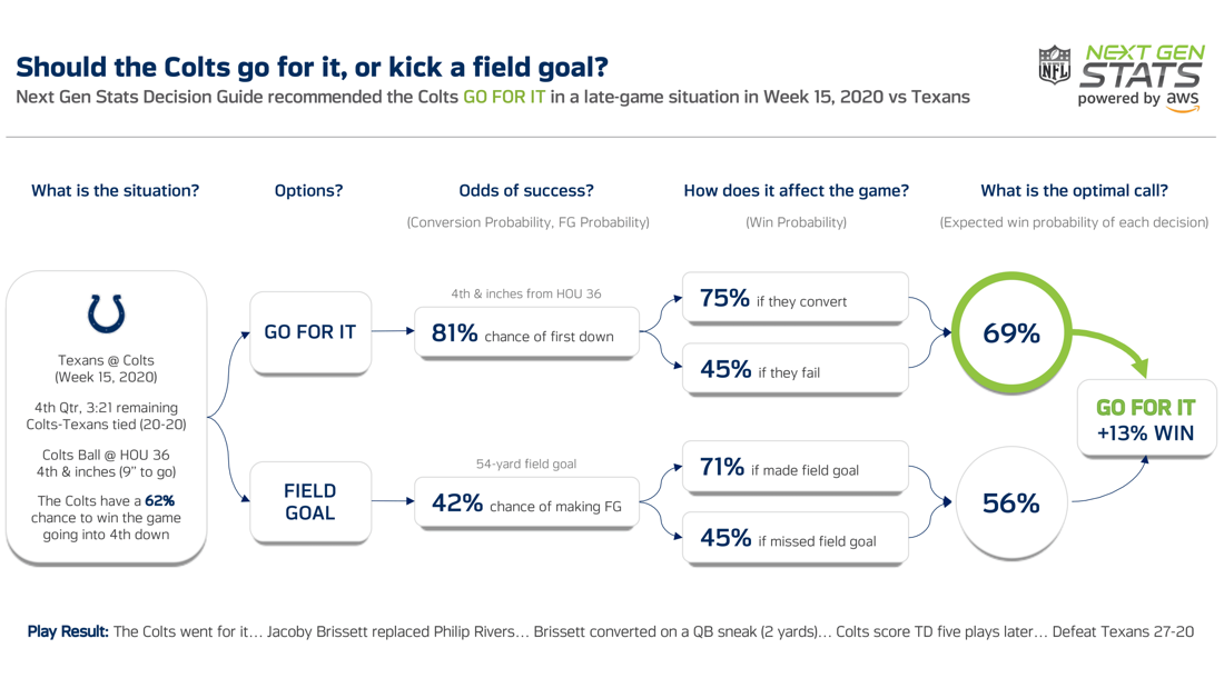
It is fourth-and-one on the Texans’ 36-yard line with 3:21 remaining on the clock in a tie game. Should the Colts’ head coach Frank Reich send out kicker Rodrigo Blankenship to attempt a 54-yard field goal or rely on his offense to convert a first down? Frank chose to go for it, leading to a first-down conversion and an eventual touchdown to seal the win. Was this the optimal call or a gamble that ended up working? Through a collaboration between the NFL’s Next Gen Stats team and AWS, NFL fans can now get an answer to this question.

Like the Colts-Texans example, the decision of what to do on a fourth down late in the game can be the difference between a win and a loss. While it can be tempting to focus on fourth-downs late in the game, even fourth-down decisions that occur early in the game can be important. Fourth-down decisions early in the game can have reverberating effects that compound over the course of a game or season. Head coaches who consistently make the right call on the fourth down put their teams in the best possible position to win, but how does a coach know what the right call is? What factors do they have to weigh, and how can a computer give fans insights into this complicated decision-making process?

The problem can be represented as a tree of choices and their respective potential outcomes. On any fourth down, a team has three main options: punt, kick a field goal, or go for it. If a team punts, their opponent generally gains possession of the ball at some point farther down the field. On a field goal attempt, the two main outcomes are the offensive team either makes the field goal or misses the field goal. If they make the field goal, they gain three points. If they miss the field goal, the defense gains possession of the ball at the location of the attempt. Similarly, if a team chooses to go for it, there are two main outcomes. Either the team gains enough yards for a first-down (or potentially a touchdown), or the defense gains possession of the ball at the end of the play.

When coaches decide what to do on a fourth-down, they must weigh all the potential outcomes and the impact of these outcomes on the odds of winning the game. To help fans understand a coach’s decision, the NFL and AWS partnered to create the Next Gen Stats Decision Guide. The Next Gen Stats Decision Guide is a suite of machine learning (ML) models designed to determine the optimal fourth-down call. The decision guide does this by predicting the odds of each potential fourth-down outcome and the resulting odds of winning the game. By comparing the odds of winning the game for each fourth-down choice, the Next Gen Stats Decision Guide provides a data-driven answer to that optimal fourth-down call.

Going back to Frank Reich’s decision, the Colts needed 0.25 yards to gain a first down. What is the probability that they convert? As shown in the following figure, our fourth-down conversion probability model predicts an 81% chance. When paired with the updated win probability of 75% if they convert, we get an expected win probability of 69%. However, if they choose to kick a field goal, the chance of making the field goal is around 42%. Paired with the win probability of 71% if successful, we get an expected win probability of 56%. Based on these expected probabilities, the Next Gen Stats Decision Guide recommends going for it with a 13% difference.

In addition to fourth-down decisions, coaches must decide what to do after scoring a touchdown. The team can kick an extra point (+1 point) or elect to attempt a two-point conversion (+2 points). The application of the Next Gen Stats Decision Guide to fourth-down plays and after-touchdown plays has been presented before, and is a good primer for this discussion. In this post, we focus on the models that determine the probability of converting a fourth-down conversion. We share how we feature engineered and developed the ML model and metrics that were used to evaluate the quality of predictions.

Go-for-it model

If a team chooses to go for it on a fourth-down, the team must gain enough yards to make a first-down on that single play. This means that not all fourth-downs are equal. Some require the offense to gain less than a yard, while others may occasionally require the offense to gain more than 10 yards. The location on the field, time left on the clock, and relative strengths of the teams are among the important parameters in understanding the odds of success. In building the Go-for-it model, we examine these and other factors to determine which features are most important in constructing a performant model.

Problem formulation

The odds of converting on a fourth-down can be formulated as a multi-class classifier. In this formulation, each class represents the offense gaining some number of yards on the play. The probability of each class is used as the odds that the team will gain that number of yards on the play. The following histogram shows the yards gained on third- and fourth-down plays from 2016–2020. An initial approach might be to make each class in the model represent an integer number of yards gained, but the histogram shows that this approach will be difficult. Classes in the long tail of the graph (roughly 40–100 yards) occur infrequently, and this sort of class imbalance can be difficult account for in model training.

To combat the potential class imbalance, we used an unequal distribution of yards to classes. Instead of each yard gained being an individual class, we used 17 different classes to encompass all the potential outcomes shown in in the graph.

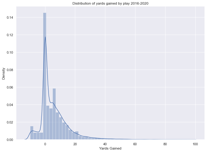
As shown in the following table, we use one class for all negative or zero-yards-gained results. Between 1–15 yards gained, we use one class for each potential outcome. The reason for this breakdown is that 88% of fourth-down plays have somewhere between 1–15 yards to go. This enables the model to capture a large majority of fourth-down situations with high fidelity. To address plays with more than 15 yards to go, we employ a decay factor to represent the decreasing probability of getting more yards on a single play.

Yards Model Classes (17)
Less than or equal to 0 0
1–15 yards 1–15 (15 classes)
16+ yards 16

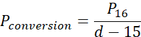
The following equation shows the decay factor used where the probability of converting ( Pconversion ) is the probability of getting 16 or more yards () divided by the actual distance needed for a first down (d ) minus 15 yards.

Features

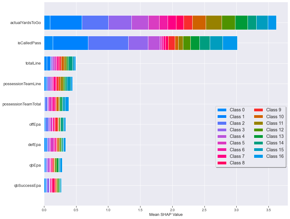
Just as a coach needs to consider many factors when deciding what to do in a game, the conversion probability models also have many potential features to use. Part of the modeling process involved determining which features to incorporate into the model. We used feature importance measures like correlation to help us identify several high-value features (see the following table). These features include the actual yards-to-go, the Vegas spread, and the historical aggregations of expected points added (EPA) by team and quarterback.

The actual yards-to-go is arguably the most important feature for this model, aligning with general football knowledge. The more yards a team needs to gain, the less likely the team is to achieve that outcome. What makes the actual yards-to-go metric even more valuable in this model is that it is derived from the NGS tracking data. Traditional NFL datasets often represent the yards-to-go as an integer, which obscures the variable nature of the game. With the NGS tracking data, we can get a measurement of the football’s location with sub-foot accuracy. This allows our model to understand the difference between fourth and inches versus fourth and 1 yard.

Although the actual yards-to-go is a clear metric to provide the model, some information is harder to quantify immediately and provide to the model. For example, a coach understands the unique skillsets of their team and the opposition, both on that day and historically. To assess coaching decisions, the model needs a way to use similar information. The Vegas lines are a useful condensation of vast amounts of situational and historical knowledge about the teams into a small set of numbers. Specifically, the point spread and the total points lines capture information about prevailing beliefs regarding the relative strengths of the teams, and the model found these values useful.

Input Features Description
actualYardsToGo The yards to go as measured using NGS tracking data between the ball at snap and the yards-to-go marker
isCalledPass Is the play predicted to be a pass or a rush?
totalLine The closing spread line for the game
possessionTeamLine The number of points the possession team is favored by according to Vegas
possessionTeamTotal The number of total points the possession team is expected to score as indicated by the Vegas total and spread lines
offEpa A team offense’s average expected points added per play over the last X number of plays in similar situations
defEpa A team defense’s average expected points added allowed per play over the last X number of plays in similar situations
qbEpa A team offense’s average expected points added per play over the last X number of plays when the quarterback on the field attempted a pass, run, or was sacked
qbSuccessEpa Quarterback success EPA for the last N similar plays

Similar to how the Vegas lines provide game-level insight into relative team strengths, we can use EPA values to provide insight into relative team strengths at a more granular level. These EPA values, calculated using other NGS models, provide insight into how the team has performed in similar situations in the past. The EPA models can be broken down by the offense, defense, and quarterback. This provides the model with information about how successful the respective teams have been in the past in addition to how successful the current quarterback has been. The following figure shows the relative importance of the features after HPO. As discussed earlier, this feature importance makes intuitive sense.

Model training

To train the model, we used all the data from third- and fourth-down plays from 2016–2019 regular seasons as the training set. We held out the data from 2020 for the testing set.

For model architecture, a handful of different models were compared, including XGBoost, PyTorch Tabular, and AutoML-based models. Of these options, the XGBoost model provided the best results. It is also explained by using the Shapely Additive Explanations (SHAP) feature importance measures. Because our goal is to optimize for conversion probabilities, we used the Brier score (probabilistic loss function) to measure the performance of our models. The Brier score measures the mean squared difference between predicted probability assigned to the possible outcomes and actual outcomes. A lower Brier score is considered better.

To optimize our models, we used Amazon SageMaker hyperparameter optimization (HPO) to fine-tune XGBoost parameters like learning rate, max depth, subsamples, alpha, and gamma. The SageMaker-managed HPO service helped us run multiple experiments in parallel to identify optimal hyperparameter configurations. Each experiment took only a few minutes because tuning jobs are distributed across 10 instances. In addition, we used SageMaker features, including automatic early stopping and warm starting from previous tuning jobs. This combined with custom metrics improved the performance of the model within minutes. Examples of various SageMaker-based HPO tuning jobs are available on GitHub.

Go-for-it model results

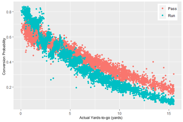
After training and HPO, the XGBoost model achieved a Brier score of 0.21. In addition to the Brier score, we examined the model predictions to ensure they were recreating known aspects of the game. For example, the odds of converting on a fourth-down play decrease as the number of yards needed for a first-down increase. The following figure shows the model’s predicted conversion probabilities as a function of the yards-to-go. We can observe two key trends. First, as expected, the conversion probability decreases as the yards-to-go increases. Second, a team is generally better off running the ball on short yards-to-go situations and passing the ball on long yards-to-go situations.

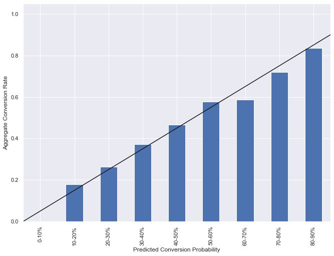
For the Next Gen Stats Decision Guide, it’s not sufficient for the model to make correct predictions. It must also assign valid probabilities to those predictions. To examine the validity of the model probabilities, we compare the probabilities against the aggregate play outcomes, as shown in the following graph. The model predictions were binned into 10%-wide categories from 0–90%. For each bin, the fraction of plays that were converted was calculated (bar height). For an ideal model, the bin heights should be roughly the midpoint of each bin (solid line). The following graph shows that when the model provides a conversion probability between 0–60%, the actual aggregate outcomes of these plays closely match the model’s predictions. For model predictions between 60–90%, the model slightly appears to underestimate the offense’s probabilities of converting (most notably between 60–70%). In situations where the agreement is poor, we can use postprocessing techniques to increase the agreement between play outcomes and the model probabilities. For an example for deep learning models, see Quantifying uncertainty in deep learning systems.

ML production pipeline

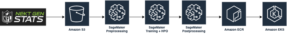
For the model in production, we used SageMaker for preprocessing, training, and postprocessing. The model is hosted using a highly scalable, available, and secured Amazon Elastic Kubernetes Service (Amazon EKS) for production usage. The following figure shows a high-level diagram of the production pipeline. All steps are automated and require minimal maintenance.

Summary

AWS and the NFL NGS team jointly developed the Next Gen Stats Decision Guide, which helps fans understand the choices coaches make at pivotal moments in the game. The odds of converting on a fourth-down play are a key component of the Next Gen Stats Decision Guide. In this post, we provided insight into how AWS helped the NFL create the model powering fourth-down conversions and discussed methods to assess model performance.

The NGS team will be hosting these models as part of the 2021 NFL season. Keep an eye out for the Next Gen Stats Decision Guide during the next NFL game.

You can find full examples of creating custom training jobs, implementing HPO, and deploying models on SageMaker at the AWS Labs GitHub repo. If you would like us to help and accelerate your use of ML, contact the Amazon ML Solutions Lab program.


About the Authors

Selvan Senthivel is a Senior ML Engineer with Amazon ML Solutions Lab team at AWS, focusing on helping customers on Machine Learning, Deep Learning problems and end-to-end ML solutions. He was the founding engineering lead of Amazon Comprehend Medical service and contributed to the design/architecture of multiple AWS AI services.

Lin Lee Cheong is a Senior Scientist and Manager with the Amazon ML Solutions Lab team at Amazon Web Services. She works with strategic AWS customers to explore and apply artificial intelligence and machine learning to discover new insights and solve complex problems.

Tyler Mullenbach is a Principal Data Science Manager with AWS Professional Services. He leads a global team of data science consultants focusing on helping customers turn their data into insights and bring ML models to production.

Ankit Tyagi is a Senior Software Engineer with the NFL’s Next Gen Stats team. He focuses on backend data pipelines and machine learning for delivering stats to fans. Outside of work, you can find him playing tennis, experimenting with brewing beer, or playing guitar.

Mike Band is the Lead Analyst for NFL’s Next Gen Stats. He contributes to the ideation, development, and communication of advanced football performance metrics for the NFL Media Group, NFL Broadcast Partners, and fans.

Juyoung Lee is a Senior Software Engineer with the NFL’s Next Gen Stats. Her work focuses on designing and developing machine learning models to create stats for fans. On her spare time, she enjoys being active by playing Ultimate Frisbee and doing CrossFit.

Michael Schaefer was the Director of Product and Analytics for NFL’s Next Gen Stats. His work focuses on the design and execution of statistics, applications, and content delivered to NFL Media, NFL Broadcaster Partners, and fans.

Michael Chi is the Director of Technology for NFL’s Next Gen Stats. He is responsible for all technical aspects of the platform which is used by all 32 clubs, NFL Media and Broadcast Partners. In his free time, he enjoys being outdoors and spending time with his family.

Read More

Chain custom Amazon SageMaker Ground Truth jobs for image processing

Amazon SageMaker Ground Truth supports many different types of labeling jobs, including several image-based labeling workflows like image-level labels, bounding box-specific labels, or pixel-level labeling. For situations not covered by these standard approaches, Ground Truth also supports custom image-based labeling, which allows you to create a labeling workflow with a completely unique UI and associated processing. Beyond that, you can chain different Ground Truth labeling jobs together so that the output of one job acts as the input to another job, to allow even more flexibility in a labeling workflow by breaking the job into multiple stages.

In this post, we show how to chain two custom Ground Truth jobs together to perform advanced image manipulations, including isolating portions of images, and de-skewing images that were photographed from an angle. Additionally, we demonstrate several techniques for augmenting source images, which are helpful for situations where you have a limited number of source images.

Extracting regions of an image

Suppose we’re tasked with creating a machine learning (ML) model that processes an image of a shelving unit and determines whether any of the bins in that shelving unit need restocking. Due to the size of the storage room, a single camera is used to capture images of several shelving units, each from a different angle. The following image is an example of such a shelving unit.

Figure 1: A shelving unit with many bins full, photographed from an angle

Figure 1: A shelving unit with many bins full, photographed from an angle

For training or inference, we need images of individual bins, rather than the overall shelving unit. The model we’re developing takes an image of a single bin, and return a classification of Empty or Full. This classification feeds into an automated restocking system, allowing us to maintain stock levels at the bin level without the trouble of someone physically checking the levels.

Unfortunately, because the shelf images are taken at an angle, each bin is skewed and has a different size and shape. Because any bin images extracted from the main image are rectangular, the extracted images include undesirable content, as shown in the following image of two adjoining bins.

Figure 2: A closeup of a single bin which shows two adjoining bins

Figure 2: A closeup of a single bin, which shows two adjoining bins

In this example, we’ve isolated a rectangular region that bounds a given bin, but because the image was taken from an angle, portions of the bins on the left and right are also partially included. Because a rectangular section includes information from other bins, an image like this performs poorly when used for training or for inference.

To solve this, we can select a non-rectangular section of the original image and warp it to create a new image. The following image demonstrates the results of a warp transformation applied to the original image.

Figure 3: Original shelving unit with just the bins isolated, and the image warped to make it orthogonal

Figure 3: Original shelving unit with just the bins isolated, and the image warped to make it orthogonal

This warping accomplishes two tasks. First, we’ve selected just the shelving unit, cropping out the nearby walls, floor, and any other irrelevant areas near the edges of the shelves. Second, the warping of the image results in each bin being more rectangular than the original version.

This warped image doesn’t have any new content—it’s just a distortion of the original image. But by performing this warping, each bin can be selected using a rectangular bounding box, which provides needed consistency, no matter what position a bin is in. Compare the following two bin images: the image on the left is extracted from the original image, and the image on the right is the same bin, extracted from the de-skewed image.

Figure 4: A single bin from the original image (left) compared with the bin from the warped image (right)

Figure 4: A single bin from the original image (left) compared with the bin from the warped image (right)

The bottom opening of the bin was originally at an angle, and now it’s horizontal. Overall, we’ve reduced the amount of the bin shown, and increased the proportion of the contents of the bin within the image. This improves our ML training process, because each bin image has less superfluous content.

Ground Truth jobs

Each custom Ground Truth labeling job is defined with a web-based user interface and two associated AWS Lambda functions (for more information, see Processing with AWS Lambda). One function runs prior to each image displayed by the UI, and the other runs after the user finishes the labeling job for all the images. Ground Truth offers several pre-made user interfaces (like bounding box-based selection), but you can also create your own custom UI if needed, as we do for this example.

When Ground Truth jobs are chained together, the output of one job is used as the input of another job. For this task, we use two chained jobs to process our images, as illustrated in the following diagram.

Figure 5: Architecture diagram showing two chained Ground Truth jobs, each with a Pre- and Post- UI Lambda function

Figure 5: Architecture diagram showing two chained Ground Truth jobs, each with a Pre- and Post- UI Lambda function

Images that need to be labeled are stored in Amazon Simple Storage Solution (Amazon S3). The first Ground Truth job retrieves images from Amazon S3 and displays them one at a time, waiting for the user to specify the four corners of the shelving unit within the image, using a custom UI. When that step is complete, the post-UI Lambda function uses the corner coordinates to warp or de-skew each image, which is then saved to the same S3 bucket that the original image resides in. Note that it’s not necessary to do this during inference—for a situation where the camera is in a fixed location, you can save those corner coordinates for later use during inference.

After the first Ground Truth job has de-skewed the source image, the second job uses simple bounding boxes to label each bin within the de-skewed image. The post-UI Lambda function then extracts the individual bin images, augments them with rotations, flipping, and color and brightness alterations, and writes the resulting data to Amazon S3, where it can be used for model training or other purposes.

You can find example code and deployment instructions in the GitHub repo.

Custom user interface

From a labeler’s perspective, after they log in and select a job, they use the custom UI to select the four corners of a bin.

Figure 6: The custom Ground Truth UI for the first labeling job

Figure 6: The custom Ground Truth UI for the first labeling job

For custom Ground Truth user interfaces, a set of custom tags is available, known as Crowd tags. These tags include bounding boxes, lines, points, and other user interface elements that you can use to build a labeling UI. In this case, we use the crowd-polygon tag, which is displayed as a yellow polygon.

After the labeler draws a polygon with four corners on the UI for all source images, they exit the UI by choosing Done. At this point, the post-UI Lambda function is run and each de-skewed image is saved to Amazon S3. When the function is complete, control is passed to the next chained Ground Truth job.

Generally, chained Ground Truth jobs reuse an output manifest file as the input manifest file for the next (chained) labeling job. In this case, we created a new image, so we modify the pre-UI Lambda function so it passes in the correct (de-skewed) file name, rather than the original, skewed image file name.

The second job in the chain uses the bounding box-based labeling functionality that is built in to Ground Truth. The bounding boxes don’t cover the entire contents of each bin, but they do cover the openings of the bins. This provides enough data to create a model to detect whether a bin is full or empty.

Figure 7: De-skewed image with bounding boxes from the second chained Ground Truth labeling job

Figure 7: De-skewed image with bounding boxes from the second chained Ground Truth labeling job

After the labeler selects all the bins, they exit the UI by choosing Done. At this point, the post-UI Lambda function runs and crops out each bin image, makes variations of it for image augmentation purposes, and saves the variations into a folder structure in Amazon S3 based on classification. The top level of the folder structure is named training_data, with two subfolders: empty and full. Each subfolder contains images of bins that are either empty or full, suitable for use in model training.

Image augmentation

Image augmentation is a technique sometimes used in image-based ML workloads. It’s especially helpful when the number of source images is low, or limited in the number of variants. Typically, image augmentation is performed by taking a source image and creating multiple variants of it, altering factors like brightness and contrast, coloring, and even cropping or rotating images. These variations help the resulting model be more robust and capable of handling images that are dissimilar to the original training images.

In this example, we use image augmentation methods in the post-UI Lambda function of the second Ground Truth job. The labeler has specified the bounding boxes for each bin image in the Ground Truth UI, and that data is used to extract portions of the overall image. Those extracted portions are of the individual bins, and these smaller images are used as input into our image augmentation process.

In our case, we create 14 variants of each bin image, with variations of brightness, contrast, and sharpness, as well horizontal flipping combined with these variations. With this approach, a single source image of a shelving unit with 24 bins generates 14 variants for each bin image, for a total of 336 images that can be used for training a model. The following shows an original bin image (upper left) and each of its variants.

Conclusion

Custom Ground Truth jobs provide a great deal of flexibility, and using them with images allows advanced functionality like cropping and de-skewing images, as well as performing custom image augmentation. The supplied Crowd HTML tags support many different labeling approaches like polygons, lines, text boxes, modal alerts, key point placement, and others. Combined with the power of pre-UI and post-UI Lambda functions, a custom Ground Truth job allows you to construct complex labeling jobs to support a wide variety of use cases, and combining different custom jobs by chaining them together provides even more options.

You can use the GitHub repo associated with this post as a starting point for your own chained image labeling jobs. You can also extend the code to support additional image augmentation methods (like cropping or rotating the source images), or modify it to fit your particular use case.

To learn more about chained Ground Truth jobs, see Chaining Labeling Jobs.

For more information about the Crowd tags you can use in the Ground Truth UI, see Crowd HTML Elements Reference.


About the Author

Greg Sommerville is a Senior Prototyping Architect on the AWS Envision Engineering Americas Prototyping team, where he helps AWS customers implement innovative solutions to challenging problems with machine learning, IoT and serverless technologies. He lives in Ann Arbor, Michigan and enjoys practicing yoga, catering to his dogs, and playing poker.

Read More

Permutation-Invariant Neural Networks for Reinforcement Learning

Posted by David Ha, Staff Research Scientist and Yujin Tang, Research Software Engineer, Google Research, Tokyo

“The brain is able to use information coming from the skin as if it were coming from the eyes. We don’t see with the eyes or hear with the ears, these are just the receptors, seeing and hearing in fact goes on in the brain.”
Paul Bach-y-Rita, quoted in Livewired

People have the amazing ability to use one sensory modality (e.g., touch) to supply environmental information normally gathered by another sense (e.g., vision). This adaptive ability, called sensory substitution, is a phenomenon well-known to neuroscience. While difficult adaptations — such as adjusting to seeing things upside-down, learning to ride a “backwards” bicycle, or learning to “see” by interpreting visual information emitted from a grid of electrodes placed on one’s tongue — require anywhere from weeks, months or even years to attain mastery, people are able to eventually adjust to sensory substitutions.

Examples of Sensory Substitution. Left: Tongue Display Unit (Maris and Bach-y-Rita, 2001; Image: Kaczmarek, 2011). Right: “Upside down goggles” initially conceived by Erismann and Kohler in 1931. (Image Wikipedia).

In contrast, most neural networks are not able to adapt to sensory substitutions at all. For instance, most reinforcement learning (RL) agents require their inputs to be in a pre-specified format, or else they will fail. They expect fixed-size inputs and assume that each element of the input carries a precise meaning, such as the pixel intensity at a specified location, or state information, like position or velocity. In popular RL benchmark tasks (e.g., Ant or Cart-pole), an agent trained using current RL algorithms will fail if its sensory inputs are changed or if the agent is fed additional noisy inputs that are unrelated to the task at hand.

In “The Sensory Neuron as a Transformer: Permutation-Invariant Neural Networks for Reinforcement Learning”, a spotlight paper at NeurIPS 2021, we explore permutation invariant neural network agents, which require each of their sensory neurons (receptors that receive sensory inputs from the environment) to figure out the meaning and context of its input signal, rather than explicitly assuming a fixed meaning. Our experiments show that such agents are robust to observations that contain additional redundant or noisy information, and to observations that are corrupt and incomplete.

Permutation invariant reinforcement learning agents adapting to sensory substitutions. Left: The ordering of the ant’s 28 observations are randomly shuffled every 200 time-steps. Unlike the standard policy, our policy is not affected by the suddenly permuted inputs. Right: Cart-pole agent given many redundant noisy inputs (Interactive web-demo).

In addition to adapting to sensory substitutions in state-observation environments (like the ant and cart-pole examples), we show that these agents can also adapt to sensory substitutions in complex visual-observation environments (such as a CarRacing game that uses only pixel observations) and can perform when the stream of input images is constantly being reshuffled:

We partition the visual input from CarRacing into a 2D grid of small patches, and shuffled their ordering. Without any additional training, our agent still performs even when the original training background (left) is replaced with new images (right).

Method
Our approach takes observations from the environment at each time-step and feeds each element of the observation into distinct, but identical neural networks (called “sensory neurons”), each with no fixed relationship with one another. Each sensory neuron integrates over time information from only their particular sensory input channel. Because each sensory neuron receives only a small part of the full picture, they need to self-organize through communication in order for a global coherent behavior to emerge.

Illustration of observation segmentation.We segment each input into elements, which are then fed to independent sensory neurons. For non-vision tasks where the inputs are usually 1D vectors, each element is a scalar. For vision tasks, we crop each input image into non-overlapping patches.

We encourage neurons to communicate with each other by training them to broadcast messages. While receiving information locally, each individual sensory neuron also continually broadcasts an output message at each time-step. These messages are consolidated and combined into an output vector, called the global latent code, using an attention mechanism similar to that applied in the Transformer architecture. A policy network then uses the global latent code to produce the action that the agent will use to interact with the environment. This action is also fed back into each sensory neuron in the next time-step, closing the communication loop.

Overview of the permutation-invariant RL method. We first feed each individual observation (ot) into a particular sensory neuron (along with the agent’s previous action, at-1). Each neuron then produces and broadcasts a message independently, and an attention mechanism summarizes them into a global latent code (mt) that is given to the agent’s downstream policy network (𝜋) to produce the agent’s action at.

Why is this system permutation invariant? Each sensory neuron is an identical neural network that is not confined to only process information from one particular sensory input. In fact, in our setup, the inputs to each sensory neuron are not defined. Instead, each neuron must figure out the meaning of its input signal by paying attention to the inputs received by the other sensory neurons, rather than explicitly assuming a fixed meaning. This encourages the agent to process the entire input as an unordered set, making the system to be permutation invariant to its input. Furthermore, in principle, the agent can use as many sensory neurons as required, thus enabling it to process observations of arbitrary length. Both of these properties will help the agent adapt to sensory substitutions.

Results
We demonstrate the robustness and flexibility of this approach in simpler, state-observation environments, where the observations the agent receives as inputs are low-dimensional vectors holding information about the agent’s states, such as the position or velocity of its components. The agent in the popular Ant locomotion task has a total of 28 inputs with information that includes positions and velocities. We shuffle the order of the input vector several times during a trial and show that the agent is rapidly able to adapt and is still able to walk forward.

In cart-pole, the agent’s goal is to swing up a cart-pole mounted at the center of the cart and balance it upright. Normally the agent sees only five inputs, but we modify the cartpole environment to provide 15 shuffled input signals, 10 of which are pure noise, and the remainder of which are the actual observations from the environment. The agent is still able to perform the task, demonstrating the system’s capacity to work with a large number of inputs and attend only to channels it deems useful. Such flexibility may find useful applications for processing a large unspecified number of signals, most of which are noise, from ill-defined systems.

We also apply this approach to high-dimensional vision-based environments where the observation is a stream of pixel images. Here, we investigate screen-shuffled versions of vision-based RL environments, where each observation frame is divided into a grid of patches, and like a puzzle, the agent must process the patches in a shuffled order to determine a course of action to take. To demonstrate our approach on vision-based tasks, we created a shuffled version of Atari Pong.

Shuffled Pong results. Left: Pong agent trained to play using only 30% of the patches matches performance of Atari opponent. Right: Without extra training, when we give the agent more puzzle pieces, its performance increases.

Here the agent’s input is a variable-length list of patches, so unlike typical RL agents, the agent only gets to “see” a subset of patches from the screen. In the puzzle pong experiment, we pass to the agent a random sample of patches across the screen, which are then fixed through the remainder of the game. We find that we can discard 70% of the patches (at these fixed-random locations) and still train the agent to perform well against the built-in Atari opponent. Interestingly, if we then reveal additional information to the agent (e.g., allowing it access to more image patches), its performance increases, even without additional training. When the agent receives all the patches, in shuffled order, it wins 100% of the time, achieving the same result with agents that are trained while seeing the entire screen.

We find that imposing additional difficulty during training by using unordered observations has additional benefits, such as improving generalization to unseen variations of the task, like when the background of the CarRacing training environment is replaced with a novel image.

Shuffled CarRacing results. The agent has learned to focus its attention (indicated by the highlighted patches) on the road boundaries. Left: Training environment. Right: Test environment with new background.

Conclusion
The permutation invariant neural network agents presented here can handle ill-defined, varying observation spaces. Our agents are robust to observations that contain redundant or noisy information, or observations that are corrupt and incomplete. We believe that permutation invariant systems open up numerous possibilities in reinforcement learning.

If you’re interested to learn more about this work, we invite readers to read our interactive article (pdf version) or watch our video. We also released code to reproduce our experiments.

Read More

A decade in deep learning, and what’s next

Twenty years ago, Google started using machine learning, and 10 years ago, it helped spur rapid progress in AI using deep learning. Jeff Dean and Marian Croak of Google Research take a look at how we’ve innovated on these techniques and applied them in helpful ways, and look ahead to a responsible and inclusive path forward.

Jeff Dean

From research demos to AI that really works

I was first introduced to neural networks — computer systems that roughly imitate how biological brains accomplish tasks — as an undergrad in 1990. I did my senior thesis on using parallel computation to train neural networks. In those early days, I thought if we could 32X more compute power (using 32 processors at the time!), we could get neural networks to do impressive things. I was way off. It turns out we would need about 1 million times as much computational power before neural networks could scale to real-world problems.

A decade later, as an early employee at Google, I became reacquainted with machine learning when the company was still just a startup. In 2001 we used a simpler version of machine learning, statistical ML, to detect spam and suggest better spellings for people’s web searches. But it would be another decade before we had enough computing power to revive a more computationally-intensive machine learning approach called deep learning. Deep learning uses neural networks with multiple layers (thus the “deep”), so it can learn not just simple statistical patterns, but can learn subtler patterns of patterns — such as what’s in an image or what word was spoken in some audio. One of our first publications in 2012 was on a system that could find patterns among millions of frames from YouTube videos. That meant, of course, that it learned to recognize cats.

To get to the helpful features you use every day — searchable photo albums, suggestions on email replies, language translation, flood alerts, and so on — we needed to make years of breakthroughs on top of breakthroughs, tapping into the best of Google Research in collaboration with the broader research community. Let me give you just a couple examples of how we’ve done this.

A big moment for image recognition

In 2012, a paper wowed the research world for making a huge jump in accuracy on image recognition using deep neural networks, leading to a series of rapid advances by researchers outside and within Google. Further advances led to applications like Google Photos in 2015, letting you search photos by what’s in them. We then developed other deep learning models to help you find addresses in Google Maps, make sense of videos on YouTube, and explore the world around you using Google Lens. Beyond our products, we applied these approaches to health-related problems, such as detecting diabetic retinopathy in 2016, and then cancerous cells in 2017, and breast cancer in 2020. Better understanding of aerial imagery through deep learning let us launch flood forecasting in 2018, now expanded to cover more than 360 million people in 2021. It’s been encouraging to see how helpful these advances in image recognition have been.

Similarly, we’ve used deep learning to accelerate language understanding. With sequence-to-sequence learning in 2014, we began looking at how to understand strings of text using deep learning. This led to neural machine translation in Google Translate in 2016, which was a massive leap in quality, particularly for less prevalent languages. We developed neural language models further for Smart Reply in Gmail in 2017, which made it easier and faster for you to knock through your email, especially on mobile. That same year, Google invented Transformers, leading to BERT in 2018, then T5, and in 2021 MUM, which lets you ask Google much more nuanced questions. And with “sparse” models like GShard, we can dramatically improve on tasks like translation while using less energy.

We’ve driven a similar arc in understanding speech. In 2012, Google used deep neural networks to make major improvements to speech recognition on Android. We kept advancing the state of the art with higher-quality, faster, more efficient speech recognition systems. By 2019, we were able to put the entire neural network on-device so you could get accurate speech recognition even without a connection. And in 2021, we launched Live Translate on the Pixel 6 phone, letting you speak and be translated in 48 languages — all on-device, while you’re traveling with no Internet.

  • image of speech-to-text on phone

    Project Relate: A communication tool for people with speech impairments.

  • image of flood forecasting map on phone

    ML-based flood forecasting helps equip those in harm’s way with accurate and detailed alerts.

  • image of mammogram

    Google Health’s AI system helps radiologistsidentify cancer in mammograms with greater accuracy.

More invention ahead

As our research goes forward, we’re balancing more immediately applied research with more exploratory fundamental research. So we’re looking at how, for example, AI can aid scientific discovery, with a project like mapping the brain of a fly, which could one day help better understand and treat mental illness in people. We’re also pursuing quantum computing, which will likely take a decade or longer to reach wide-scale applications. This is why we publish nearly1000 papers a year, including around 200 related to responsible AI, and we’ve given over 6500 grants to external researchers over the past decade and a half.

Looking ahead from 2021 to 2031, I’m excited about the next-generation AI systems we can build, and how much more helpful they’ll be. We’re planting the seeds today with new architectures like Pathways, with more to come.

Marian Croak

Minding the gap(s)

As we develop these lines of research and turn them into useful technologies, we’re mindful of the broader societal impact of AI, and especially that technology has not always had an equitable impact. This is personal for me — I care deeply about ensuring that people from all different backgrounds and circumstances have a good experience.

So we’re increasing the depth and rigor of how we review and evaluate our research to ensure we’re developing it responsibly. We’re also scaling up what we learn by inventing new tools to understand and calibrate critical AI systems across Google’s products. We’re growing our organization to 200 experts in Responsible AI and Human Centered Technology, and working with hundreds of partners in product, privacy, security, and other teams across Google.

As one example of our work on responsible AI, Google Research began exploring the nascent field of ML fairness in 2016. The teams realized that on top of publishing papers, they could have a greater impact by teaching ML practitioners how to build with fairness in mind, as with the course we launched in 2018. We also started building interactive tools that coders and researchers could use, from the What-If Tool in 2018 to the 2019 launch of our Fairness Indicators tool, all the way to Know Your Data in 2021. All of these are concrete ways that AI developers can test their datasets and models to see what kind of biases and gaps there are, and start to work on mitigations to prevent unfair outcomes.

A principled approach

In fact, fairness is one of the key tenets of our AI Principles. We developed these principles in 2017 and published them in 2018, announcing not only the Principles themselves but a set of responsible AI practices with practical organizational and technical advice from what we’ve learned along the way. I was proud to be involved in the AI Principles review process from early on — I’ve seen firsthand how rigorous the teams at Google are on evaluating the technology we’re developing and deciding how best to deploy it in the real world.

Indeed, there are paths we’ve chosen not to go down — the AI Principles describe a number of areas we avoid. In line with our principles, we’ve taken a very cautious approach on face recognition. We recognize how fraught this area is not only in terms of privacy and surveillance concerns, but also its potential for unfair bias and impacts on historically marginalized groups. I’m glad that we’re taking this so thoughtfully and carefully.

We’re also developing technologies that help engineers apply the AI Principles directly — for example, incorporating privacy design principles. We invented Federated Learning in 2017 as a way to train ML models without your personal data leaving your phone. In 2018 we showed how well this works on Gboard, the free keyboard you can download for your phone — it learns to provide you more useful suggestions, while keeping what you type private on your device.

If you’re curious, you can learn more about all these veins of research, product impact, processes, and external engagement in our 2021 AI Principles Progress Update.

AI by everyone, for everyone

As we look to the decade ahead, it’s incredibly important that AI be built in a way that works well for everyone. That means building as inclusive a team as we can ourselves at Google. It also means ensuring the field as a whole increasingly represents the people whose lives it aims to improve.

I’m proud to lead the Black Leadership Advisory Group (BLAG) at Google. We helped craft and drive programs included in Google’s recent update on racial equity work. For example, we paired up new director-level hires with BLAG members, and the feedback has been really positive, with 80% of respondents saying they’d recommend the program. We’re looking at extending this to other groups, including for Latinx+ and Asian+ Googlers. We’re holding ourselves accountable as leaders too — we now evaluate all VPs and above at Google on progress on diversity, equity, and inclusion. This is crucial if we’re going to have a more representative set of researchers and engineers building future technologies.

For the broader research and computer science communities, we’re providing a wide variety of grants, programs, and collaborations that we hope will welcome a more representative range of researchers. Our Research Scholar Program, begun in 2021, gave grants to more than 50 universities in 15+ countries — and 43% of the principal investigators identify as part of a group that’s been historically marginalized in tech. Similarly, our exploreCSR and CS Research Mentorship programs support thousands of undergrads from marginalized groups. And we’re partnering with groups like the National Science Foundation on their new Institute for Human-AI Collaborations.

We’re doing everything we can to make AI work well for all people. We’ll not only help ensure products across Google are using the latest practices in responsible AI — we’ll also encourage new products and features that serve those who’ve historically missed out on helpful new technologies. One example is Project Relate, which uses machine learning to help people with speech impairments communicate and use technology more easily. Another is Real Tone, which helps our imaging products like our Pixel phone camera and Google Photos more accurately and beautifully represent a diverse range of skin tones. These are just the start.

We’re excited for what’s ahead in AI, for everyone.

Read More

Introducing TensorFlow Graph Neural Networks

Posted by Sibon Li, Jan Pfeifer and Bryan Perozzi and Douglas Yarrington

Today, we are excited to release TensorFlow Graph Neural Networks (GNNs), a library designed to make it easy to work with graph structured data using TensorFlow. We have used an earlier version of this library in production at Google in a variety of contexts (for example, spam and anomaly detection, traffic estimation, YouTube content labeling) and as a component in our scalable graph mining pipelines. In particular, given the myriad types of data at Google, our library was designed with heterogeneous graphs in mind. We are releasing this library with the intention to encourage collaborations with researchers in industry.

Why use GNNs?

Graphs are all around us, in the real world and in our engineered systems. A set of objects, places, or people and the connections between them is generally describable as a graph. More often than not, the data we see in machine learning problems is structured or relational, and thus can also be described with a graph. And while fundamental research on GNNs is perhaps decades old, recent advances in the capabilities of modern GNNs have led to advances in domains as varied as traffic prediction, rumor and fake news detection, modeling disease spread, physics simulations, and understanding why molecules smell.

Graphs can model the relationships between many different types of data, including web pages (left), social connections (center), or molecules (right).

A graph represents the relations (edges) between a collection of entities (nodes or vertices). We can characterize each node, edge, or the entire graph, and thereby store information in each of these pieces of the graph. Additionally, we can ascribe directionality to edges to describe information or traffic flow, for example.

GNNs can be used to answer questions about multiple characteristics of these graphs. By working at the graph level, we try to predict characteristics of the entire graph. We can identify the presence of certain “shapes,” like circles in a graph that might represent sub-molecules or perhaps close social relationships. GNNs can be used on node-level tasks, to classify the nodes of a graph, and predict partitions and affinity in a graph similar to image classification or segmentation. Finally, we can use GNNs at the edge level to discover connections between entities, perhaps using GNNs to “prune” edges to identify the state of objects in a scene.

Structure

TF-GNN provides building blocks for implementing GNN models in TensorFlow. Beyond the modeling APIs, our library also provides extensive tooling around the difficult task of working with graph data: a Tensor-based graph data structure, a data handling pipeline, and some example models for users to quickly onboard.

The various components of TF-GNN that make up the workflow.

The initial release of the TF-GNN library contains a number of utilities and features for use by beginners and experienced users alike, including:

  • A high-level Keras-style API to create GNN models that can easily be composed with other types of models. GNNs are often used in combination with ranking, deep-retrieval (dual-encoders) or mixed with other types of models (image, text, etc.)
    • GNN API for heterogeneous graphs. Many of the graph problems we approach at Google and in the real world contain different types of nodes and edges. Hence we chose to provide an easy way to model this.
  • A well-defined schema to declare the topology of a graph, and tools to validate it. This schema describes the shape of its training data and serves to guide other tools.
  • A GraphTensor composite tensor type which holds graph data, can be batched, and has graph manipulation routines available.
  • A library of operations on the GraphTensor structure:
    • Various efficient broadcast and pooling operations on nodes and edges, and related tools.
    • A library of standard baked convolutions, that can be easily extended by ML engineers/researchers.
    • A high-level API for product engineers to quickly build GNN models without necessarily worrying about its details.
  • An encoding of graph-shaped training data on disk, as well as a library used to parse this data into a data structure from which your model can extract the various features.

Example usage

In the example below, we build a model using the TF-GNN Keras API to recommend movies to a user based on what they watched and genres that they liked.

We use the ConvGNNBuilder method to specify the type of edge and node configuration, namely to use WeightedSumConvolution (defined below) for edges. And for each pass through the GNN, we will update the node values through a Dense interconnected layer:

    import tensorflow as tf
import tensorflow_gnn as tfgnn

# Model hyper-parameters:
h_dims = {'user': 256, 'movie': 64, 'genre': 128}

# Model builder initialization:
gnn = tfgnn.keras.ConvGNNBuilder(
lambda edge_set_name: WeightedSumConvolution(),
lambda node_set_name: tfgnn.keras.layers.NextStateFromConcat(
tf.keras.layers.Dense(h_dims[node_set_name]))
)

# Two rounds of message passing to target node sets:
model = tf.keras.models.Sequential([
gnn.Convolve({'genre'}), # sends messages from movie to genre
gnn.Convolve({'user'}), # sends messages from movie and genre to users
tfgnn.keras.layers.Readout(node_set_name="user"),
tf.keras.layers.Dense(1)
])

The code above works great, but sometimes we may want to use a more powerful custom model architecture for our GNNs. For example, in our previous use case, we might want to specify that certain movies or genres hold more weight when we give our recommendation. In the following snippet, we define a more advanced GNN with custom graph convolutions, in this case with weighted edges. We define the WeightedSumConvolution class to pool edge values as a sum of weights across all edges:

class WeightedSumConvolution(tf.keras.layers.Layer):
"""Weighted sum of source nodes states."""

def call(self, graph: tfgnn.GraphTensor,
edge_set_name: tfgnn.EdgeSetName) -> tfgnn.Field:
messages = tfgnn.broadcast_node_to_edges(
graph,
edge_set_name,
tfgnn.SOURCE,
feature_name=tfgnn.DEFAULT_STATE_NAME)
weights = graph.edge_sets[edge_set_name]['weight']
weighted_messages = tf.expand_dims(weights, -1) * messages
pooled_messages = tfgnn.pool_edges_to_node(
graph,
edge_set_name,
tfgnn.TARGET,
reduce_type='sum',
feature_value=weighted_messages)
return pooled_messages

Note that even though the convolution was written with only the source and target nodes in mind, TF-GNN makes sure it’s applicable and works on heterogeneous graphs (with various types of nodes and edges) seamlessly.

Next steps

You can check out the TF-GNN GitHub repo for more information. To stay up to date, you can read the TensorFlow blog, join the TensorFlow Forum at discuss.tensorflow.org, follow twitter.com/tensorflow, or subscribe to youtube.com/tensorflow. If you’ve built something you’d like to share, please submit it for our Community Spotlight at goo.gle/TFCS. For feedback, please file an issue on GitHub. Thank you!

Acknowledgments

The work described here was a research collaboration between Oleksandr Ferludin‎, Martin Blais, Jan Pfeifer‎, Arno Eigenwillig, Dustin Zelle, Bryan Perozzi and Da-Cheng Juan of Google, and Sibon Li, Alvaro Sanchez-Gonzalez, Peter Battaglia, Kevin Villela, Jennifer She and David Wong of DeepMind.

Read More

From Process to Product Design: How Rendermedia Elevates Manufacturing Workflows With XR Experiences

Manufacturers are bringing product designs to life in a newly immersive world.

Rendermedia, based in the U.K., specializes in immersive solutions for commerce and industries. The company provides clients with tools and applications for photorealistic virtual, augmented and extended reality (collectively known as XR) in areas like product design, training and collaboration.

With NVIDIA RTX graphics and NVIDIA CloudXR, Rendermedia helps businesses get their products in the hands of customers and audiences, allowing them to interact and engage collaboratively on any device, from any location.

Expanding XR Spaces With CloudXR

Previously, Rendermedia could only deliver realistic rendered products to customers through a CG rendered film, which was often time-consuming to create. It also didn’t allow for consumers to dynamically interact with the product.

With NVIDIA CloudXR, Rendermedia and its product manufacturing clients can quickly render and create fully interactive simulated products in photographic detail, while also reducing their time to market.

This can be achieved by transforming raw product computer-aided design (CAD) into a realistic digital twin of the product. The digital twin can then be used across the entire organization, from sales and marketing to health and safety teams.

Rendermedia can also use CloudXR to offer organizations the ability to design, market, sell and train different teams and customers around their products in different languages worldwide.

“With both the range of 3D data evolving and devices enabling us to interact with products and environments in scale, this ultimately drives the demands around the complexity and sophistication across products and environments within an organization,” said Rendermedia founder Mark Miles.

Rendermedia customers Airbus and National Grid are using VR experiences to showcase future products and designs in realistic scenarios.

Airbus, which designs, manufactures and sells aerospace products worldwide, has worked with Rendermedia on over 35 virtual experiences. Recently, Rendermedia helped bring Airbus’ vision to life by creating VR experiences that allowed users to experience its newest products in complete context and at scale.

National Grid is an electricity and gas utility company headquartered in the U.K. With the help of Rendermedia, National Grid used photorealistic digital twins of real-life industrial sites for virtual training for employees.

The power of NVIDIA CloudXR and RTX technology allows product manufacturers to visualize designs and 3D models using Rendermedia’s platform with more realism. And they can easily make changes to designs in real time, helping users iterate more often and get to final product designs quicker. CloudXR is cost-efficient and provides common standards for training across every learner.

“CloudXR combined with RTX means that our customers can virtualize any part of their business and access it on any device at scale,” said Miles. “This is especially important in training, where the abundance of platforms and devices that people consume can vary widely. CloudXR means that any training content can be consumed at the same level of detail, so content does not have to be readapted for different devices.”

With NVIDIA CloudXR, Rendermedia can further push the boundaries of photorealistic graphics in immersive environments, all without worrying about delivering to different devices and audiences.

Learn more about NVIDIA CloudXR and how it can enhance workflows.

And catch up on a few NVIDIA GTC sessions to see how other companies are using CloudXR.

The post From Process to Product Design: How Rendermedia Elevates Manufacturing Workflows With XR Experiences appeared first on The Official NVIDIA Blog.

Read More