Create and manage Amazon EMR Clusters from SageMaker Studio to run interactive Spark and ML workloads – Part 2

In Part 1 of this series, we offered step-by-step guidance for creating, connecting, stopping, and debugging Amazon EMR clusters from Amazon SageMaker Studio in a single-account setup.

In this post, we dive deep into how you can use the same functionality in certain enterprise-ready, multi-account setups. As described in the AWS Well-Architected Framework, separating workloads across accounts enables your organization to set common guardrails while isolating environments. This can be particularly useful for certain security requirements, as well as simplify cost between projects and teams.

Solution overview

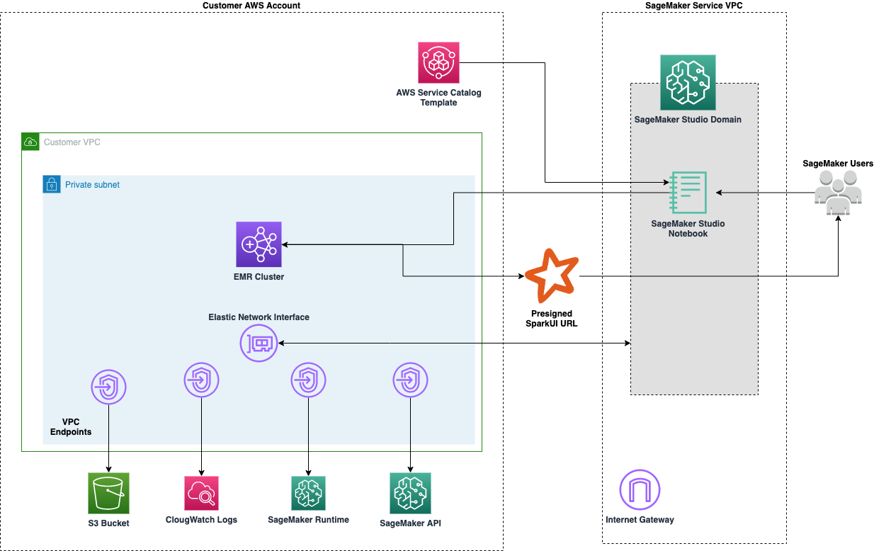
In this post, we go through the process to achieve the following architectural setup. We present the same simple interface as we saw in Part 1 for our data workers, abstracting away multi-account details from their day-to-day workflow when not needed.

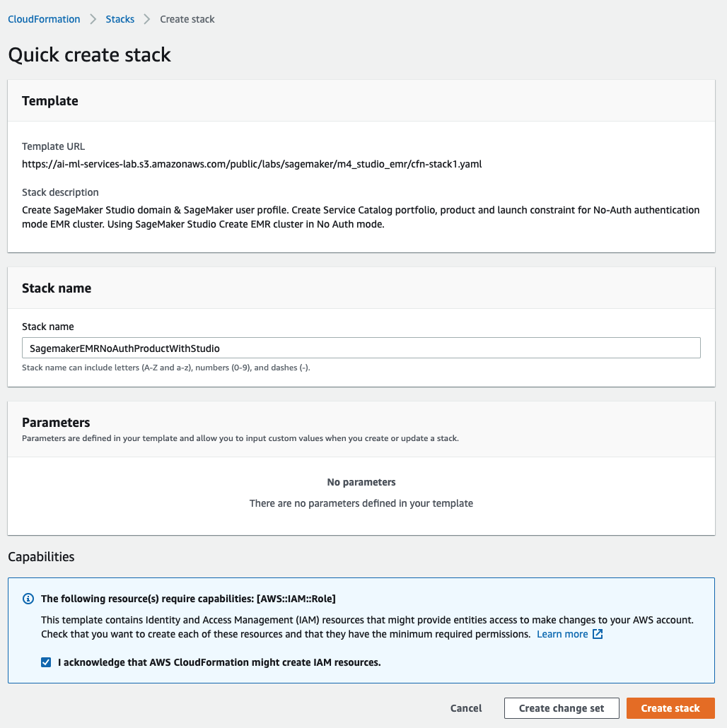
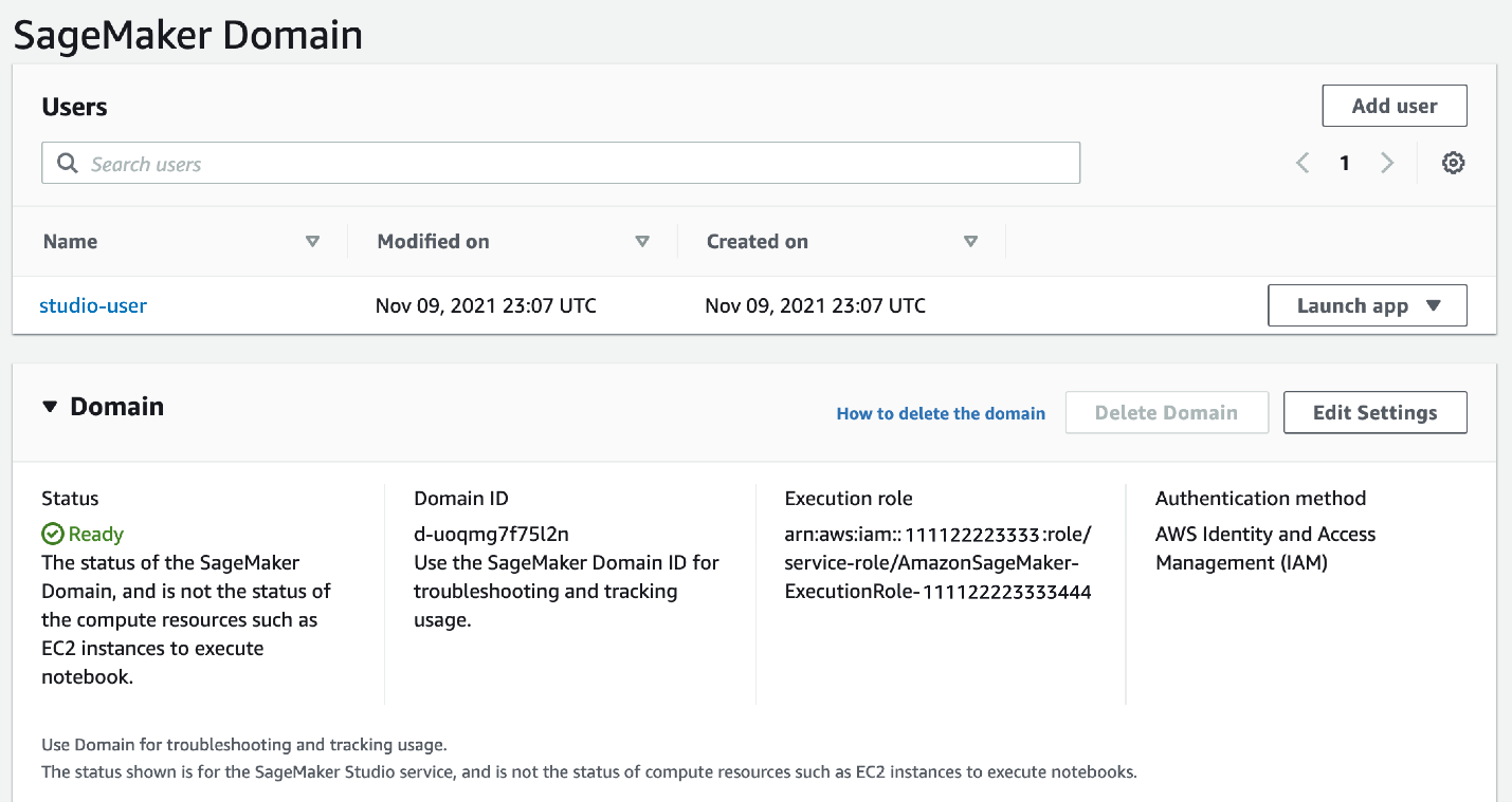
We first describe how to set up your cross-account networks in order to connect to Amazon EMR from Studio. To start, we need to make sure that some prerequisites are set correctly. For our example, a DevOps admin needs to configure an Amazon SageMaker domain with an elastic network interface to a private VPC and specify the security group ID to attach.

Set up the network

After we set up the Studio domain, we need to configure our network settings to allow communication between accounts.

VPC peering

We start with VPC peering between the accounts in order to facilitate traffic back and forth.

  1. From our Studio account, on the Amazon Virtual Private Cloud (Amazon VPC) console, choose Peering connections.
  2. Choose Create peering connection.
  3. Create your request to peer the Studio VPC within the Amazon EMR account’s VPC.

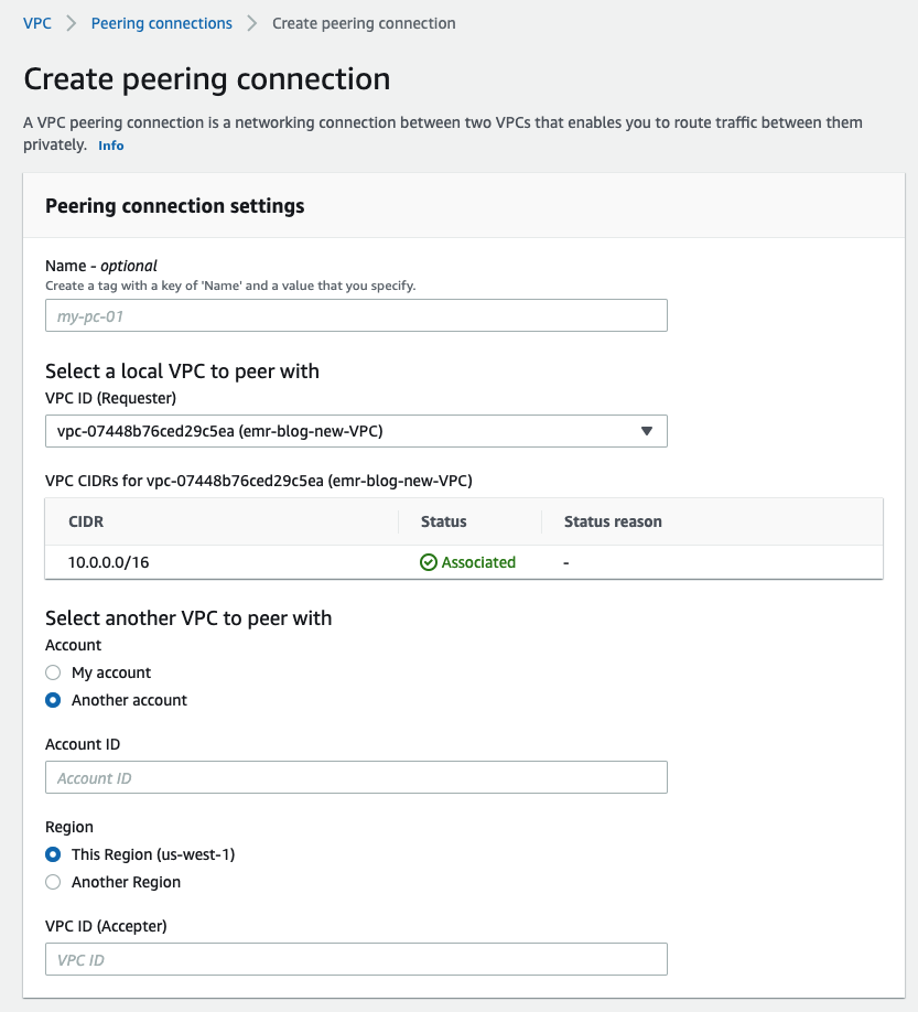
After you make the peering request, the admin can accept this request from the second account.

When peering private subnets, you should enable private IP DNS resolution at the VPC peering connection level.

Route tables

After you establish the peering connection, you must enable the flow of traffic by manually adding routes to the private subnet route tables in both accounts. We do this to enable creation and connection of EMR clusters from the Studio account to the remote account’s private subnet.

These routes point to the IP address range of the peered VPC’s private subnets and are set by going to the Route Tables tab found on the subnet page. Here the admin on each account can edit the routes.

The following route table of a Studio subnet shows traffic outbound from the Studio account for 2.0.1.0/24 through a peering connection.

The following route table of an Amazon EMR subnet shows traffic outbound from the Amazon EMR account to Studio for 10.0.20.0/24 through a peering connection.

Security groups

Lastly, the security group that is attached to your Studio domain must allow outbound traffic, and the security group of the Amazon EMR primary node must allow inbound TCP traffic from the Studio instance security group.

The following screenshot shows the inbound rules configuration in your SageMaker account.

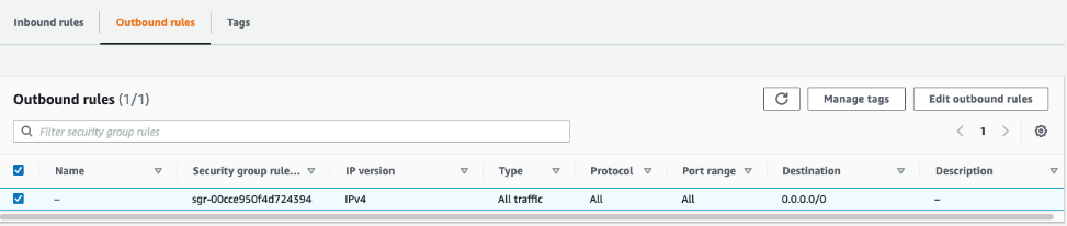
The following screenshot shows the inbound rules configuration in your Amazon EMR account.
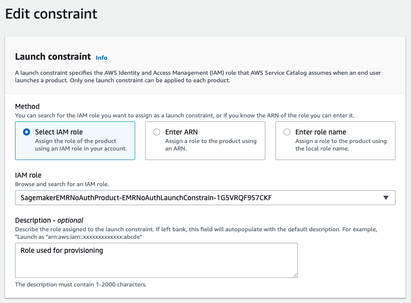
Set up permissions

We need to create an AWS Identity and Access Management (IAM) role in the secondary Amazon EMR account that has the same Amazon EMR visibility permission as we saw in Part 1.

The following code shows the specific permissions for the IAM role. It’s the same as in Part 1, but includes the policy AllowRoleAssumptionForCrossAccountDiscovery:

{
    "Version": "2012-10-17",
    "Statement": [
        {
            "Sid": "AllowPresignedUrl",
            "Effect": "Allow",
            "Action": [
                "elasticmapreduce:DescribeCluster",
                "elasticmapreduce:ListInstanceGroups",
                "elasticmapreduce:CreatePersistentAppUI",
                "elasticmapreduce:DescribePersistentAppUI",
                "elasticmapreduce:GetPersistentAppUIPresignedURL",
                "elasticmapreduce:GetOnClusterAppUIPresignedURL"
            ],
            "Resource": [
                "arn:aws:elasticmapreduce:<region>:<account-id>:cluster/*"
            ]
        },
        {
            "Sid": "AllowClusterDetailsDiscovery",
            "Effect": "Allow",
            "Action": [
                "elasticmapreduce:DescribeCluster",
                "elasticmapreduce:ListInstanceGroups"
            ],
            "Resource": [
                "arn:aws:elasticmapreduce:<region>:<account-id>:cluster/*"
            ]
        },
        {
            "Sid": "AllowClusterDiscovery",
            "Effect": "Allow",
            "Action": [
                "elasticmapreduce:ListClusters"
            ],
            "Resource": "*"
        },
        { 
            "Sid": "AllowRoleAssumptionForCrossAccountDiscovery", 
            "Effect": "Allow", 
            "Action": "sts:AssumeRole", 
            "Resource": ["arn:aws:iam::<cross-account>:role/<studio-execution-role>" ]
        },
        {
            "Sid": "AllowEMRTemplateDiscovery",
            "Effect": "Allow",
            "Action": [
              "servicecatalog:SearchProducts"
            ],
            "Resource": "*"
        }
    ]
}

This assumable role also needs a trust relationship with the Studio account (be sure to modify the account ID):

{
  "Version": "2012-10-17",
  "Statement": [
    {
      "Effect": "Allow",
      "Principal": {
        "AWS": "arn:aws:iam::<account-id>:root"
      },
      "Action": "sts:AssumeRole"
    }
  ]
}

User journey

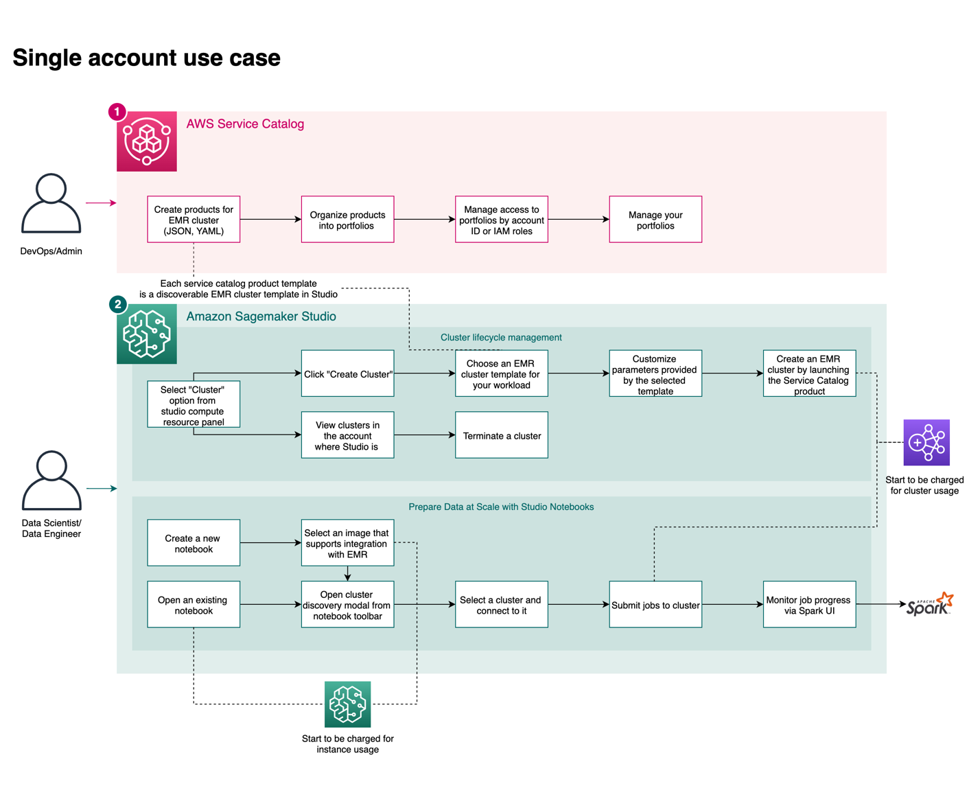
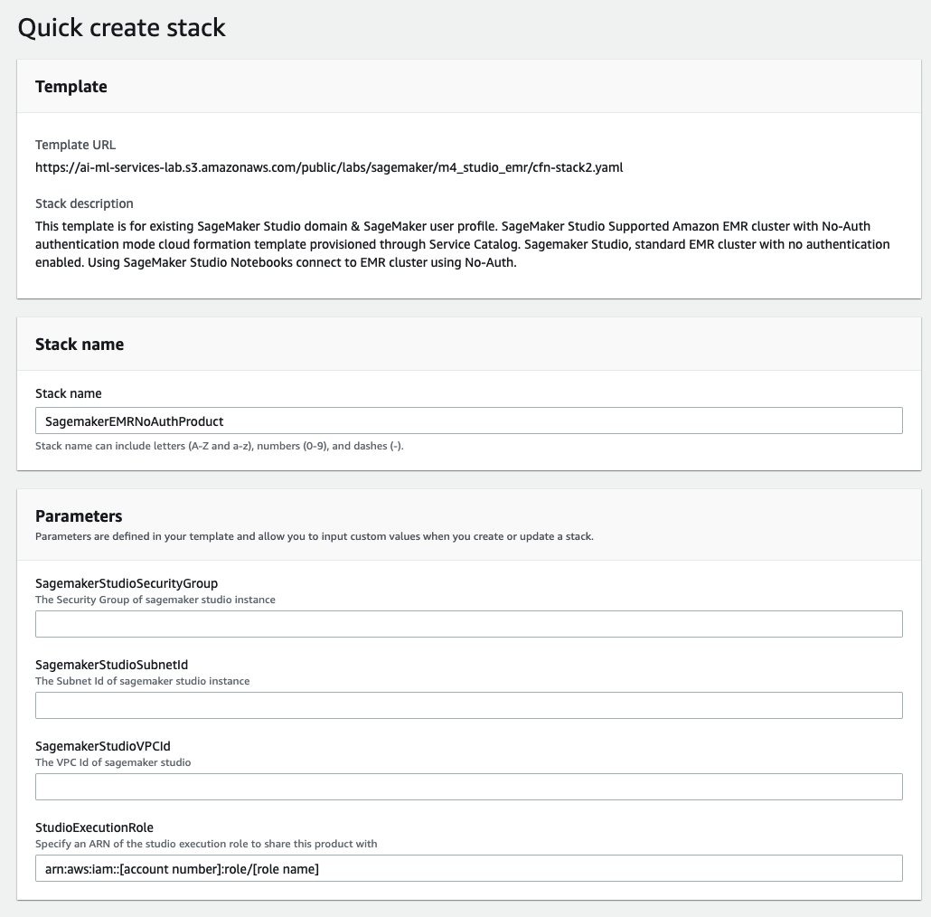
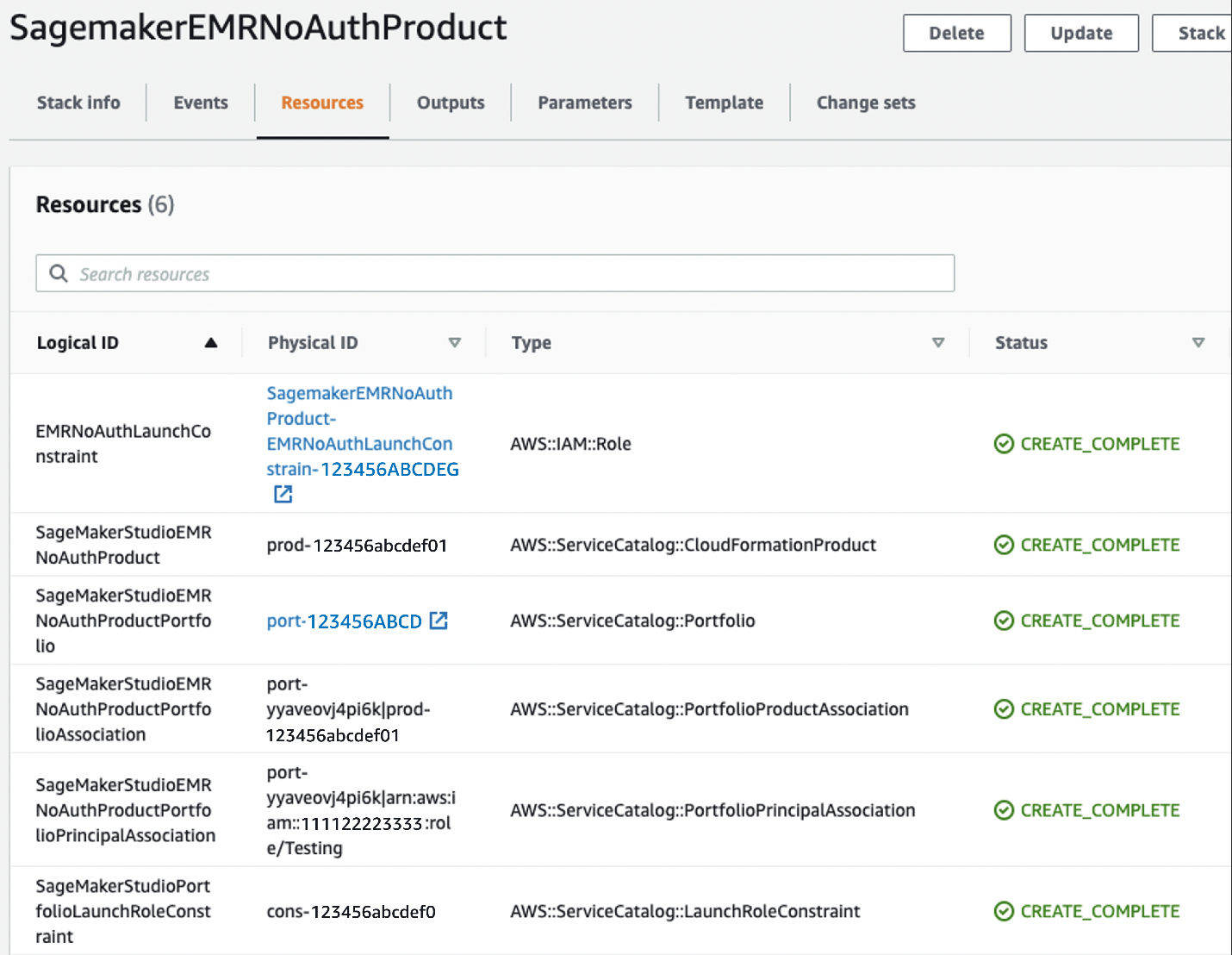
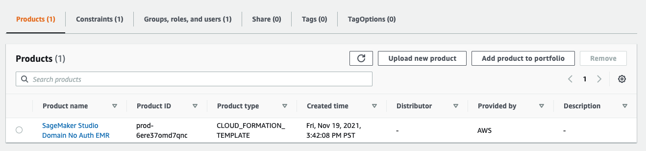
The following diagram illustrates the user journey for a unified notebook experience after you connect your various accounts. Just as in the previous post, the DevOps persona creates an AWS Service Catalog product and portfolio within the Studio account, from which data workers can provision templated EMR clusters.

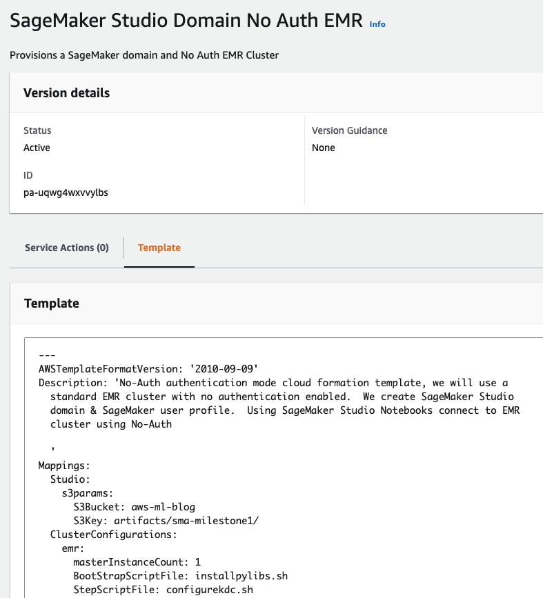
Again, it’s worth noting that you can modify the full set of properties for Amazon EMR when creating AWS CloudFormation templates that can be deployed though Studio. This means that you can enable Spot, auto scaling, and other popular configurations through your Service Catalog product.

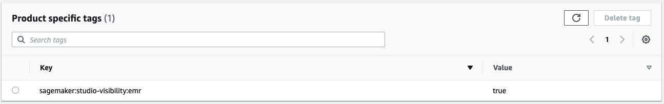
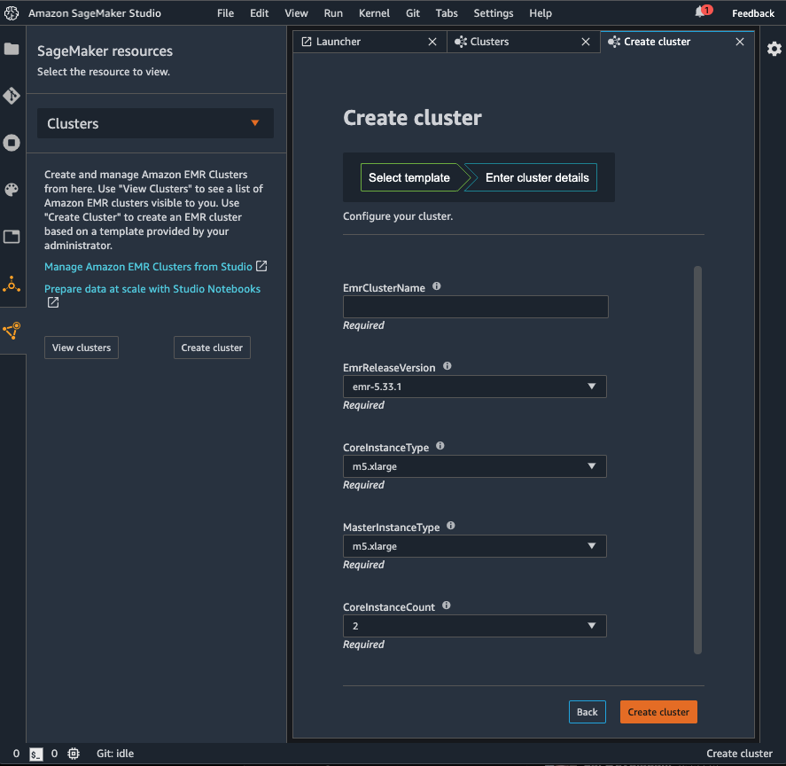
You can parameterize the preset CloudFormation template, which creates the EMR cluster, so that end-users can modify different aspects of the cluster to match their workloads. For example, the data scientist or data engineer may want to specify the number of core nodes on the cluster, and the creator of the template can specify AllowedValues to set guardrails.

Discover EMR clusters across accounts

To enable cluster discovery across accounts, we need to provide the previously created remote IAM role ARN to the Studio execution role. The Studio execution role assumes that remote role to discover and connect to EMR clusters in the remote account. The ARN of this assumable cross-account role is loaded by the Studio Jupyter server at launch and determines which role to use for cross-account cluster discoverability. To set and modify these user-specific ARNs, admins can create a Lifecycle Configuration (LCC), associated with the Jupyter server not the kernel gateway app, which writes the role ARN onto the Amazon Elastic File System (Amazon EFS) home directory for each user. You can apply this LCC to the entire set of users or it can be specific to individuals so they have granular access to which clusters can be viewed through assumed roles.

When the Jupyter server starts, lifecycle configurations run prior to reading of ARN roles that are written in the config file. This enables administrators to overwrite and fully control which cross-account ARNs are used at runtime. After the LCC runs and the files are written, the server reads the file /home/sagemaker-user/.cross-account-configuration-DO_NOT_DELETE/emr-discovery-iam-role-arns-DO_NOT_DELETE.json and stores that cross-account ARN. The following is an example LCC bash script:

# This script creates the file that informs SageMaker Studio that the role "arn:aws:iam::123456789012:role/ASSUMABLE-ROLE" in remote account "123456789012" must be assumed to list and describe EMR clusters in the remote account.

#!/bin/bash

set -eux

FILE_DIRECTORY="/home/sagemaker-user/.cross-account-configuration-DO_NOT_DELETE"
FILE_NAME="emr-discovery-iam-role-arns-DO_NOT_DELETE.json"
FILE="$FILE_DIRECTORY/$FILE_NAME"

mkdir -p $FILE_DIRECTORY

cat > "$FILE" <<- "EOF"
{
  "123456789012": "arn:aws:iam::123456789012:role/ASSUMABLE-ROLE"
}
EOF

At this point, a user can log in to their account and although they can modify this file, there’s no impact to the admin’s ARN designation. This is because the value is already stored by this point and the file is overwritten upon the server being restarted, because the LCC runs every time the Jupyter server app is started.

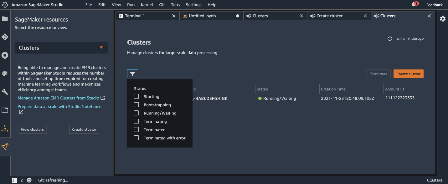
This configuration process can be completely abstracted away from data workers who discover and connect to clusters within the Studio. The only noticeable difference for cross-account clusters is that on the browsing tab, there is a column for account ID for which the cluster is housed in.

Use EMR clusters across accounts

After you establish cross-account visibility, the process for creating and stopping clusters remains the same as in Part 1. Refer to our GitHub repository for example cross-account CloudFormation stacks.

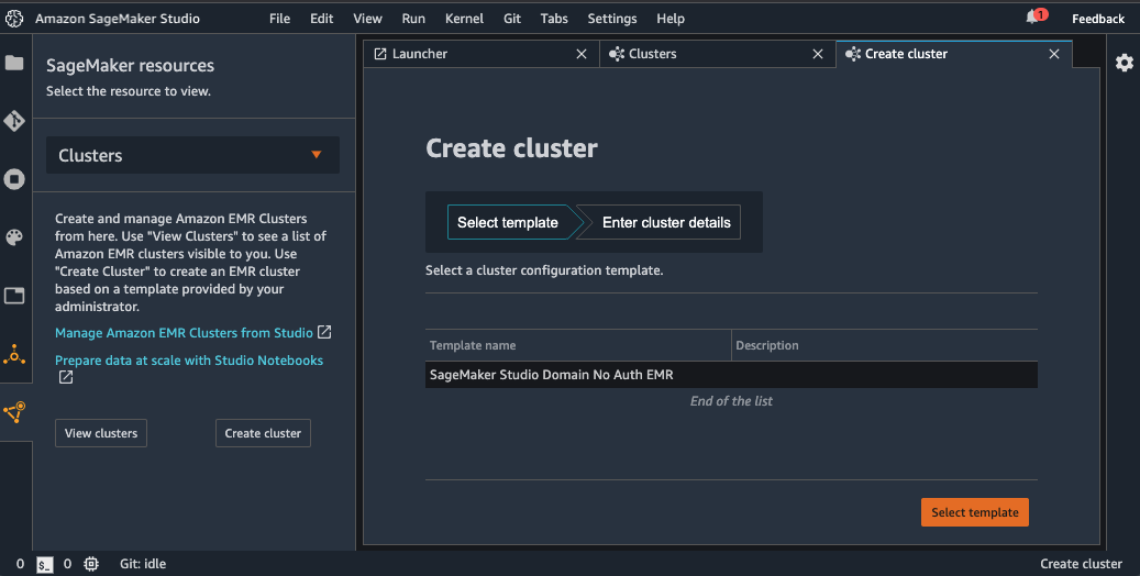
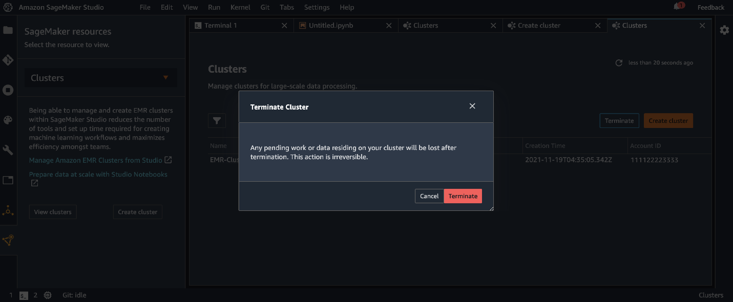
After you deploy the Service Catalog product, the process for end-users to spin up a cluster remains the same. Simply go to the Clusters page and choose Create cluster.

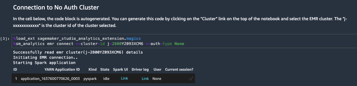
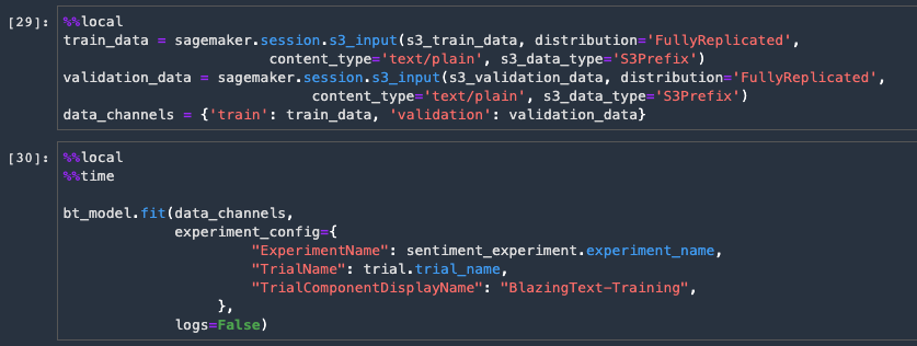
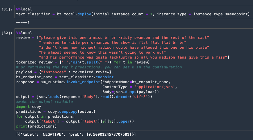
After cluster creation, we connect to our cluster using the Clusters graphical interface in Studio Notebooks. This creates an auto-populated magic cell that appears largely the same as with a single account, but with an appended parameter for the assumable cross-account role.

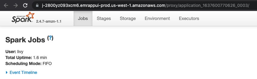
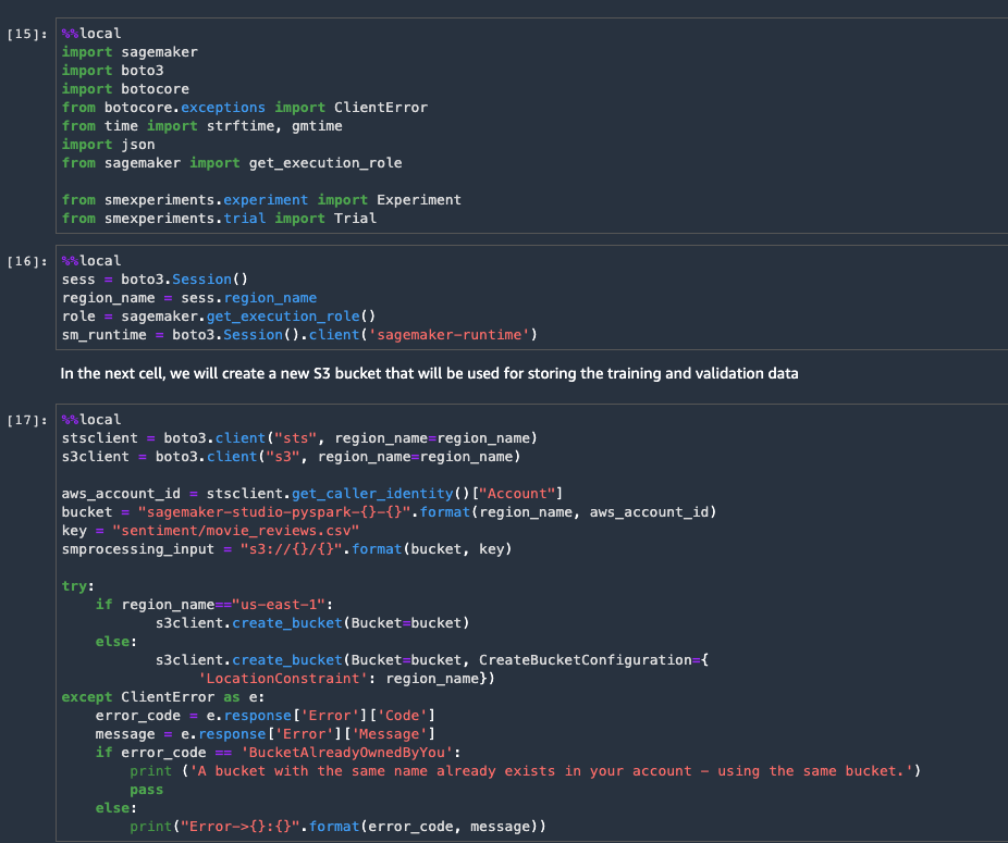
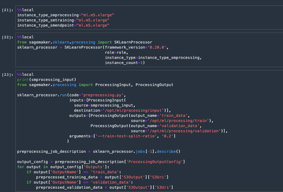
After the connection is made, we can proceed with the demo as before. You can clone our GitHub example repo and run through the notebook example just as in Part 1.

Conclusion

In this second and final part of our series, we showed how Studio users can create, connect, debug, and stop EMR clusters in cross-account setups. After you set up the networking and permissions, the end-user experience is just as we saw in Part 1. We encourage you to utilize this new functionality of Studio in your multi-account workloads today!


About the Authors

Sumedha Swamy is a Principal Product Manager at Amazon Web Services. He leads SageMaker Studio team to build it into the IDE of choice for interactive data science and data engineering workflows. He has spent the past 15 years building customer-obsessed consumer and enterprise products using Machine Learning. In his free time he likes photographing the amazing geology of the American Southwest.

Prateek Mehrotra is a Senior SDE working for SageMaker Studio at Amazon Web Services. He is focused on building interactive ML solutions which simplify usability by abstracting away complexity. In his spare time, Prateek enjoys spending time with his family and likes to explore the world with them.

Sriharsha M S is an AI/ML specialist solutions architect in the Strategic Specialist team at Amazon Web Services. He works with strategic AWS customers who are taking advantage of AI/ML to solve complex business problems. He provides technical guidance and design advice to implement AI/ML applications at scale. His expertise spans application architecture, big data, analytics, and machine learning.

Sean MorganSean Morgan is a Senior ML Solutions Architect at AWS. He has experience in the semiconductor and academic research fields, and uses his experience to help customers reach their goals on AWS. In his free time Sean is an activate open source contributor/maintainer and is the special interest group lead for TensorFlow Addons.

Ruchir Tewari is a Senior Solutions Architect specializing in security and is a member of the ML TFC. For several years he has helped customers build secure architectures for a variety of hybrid, big data and AI/ML applications. He enjoys spending time with family, music and hikes in nature.

Luna Wang is a UX designer at AWS who has a background in computer science and interaction design. She is passionate about building customer-obsessed products and solving complex technical and business problems by using design methods. She is now working with a cross-functional team to build a set of new capabilities for interactive ML in SageMaker Studio.

Read More

Create and manage Amazon EMR Clusters from SageMaker Studio to run interactive Spark and ML workloads – Part 1

Amazon SageMaker Studio is the first fully integrated development environment (IDE) for machine learning (ML). It provides a single, web-based visual interface where you can perform all ML development steps required to prepare data, as well as build, train, and deploy models. We recently introduced the ability to visually browse and connect to Amazon EMR clusters right from the Studio notebook. Starting today, you can now monitor and debug your Spark jobs running on Amazon EMR from Studio notebooks with just a single click. Additionally, you can now discover, connect to, create, stop, and manage EMR clusters directly from Studio.

We demonstrate these newly introduced capabilities in this two-part post.

Analyzing, transforming, and preparing large amounts of data is a foundational step of any data science and ML workflow. Data workers such as data scientists and data engineers use Apache Spark, Hive, and Presto running on Amazon EMR for fast data preparation. Until today, these data workers could easily discover and connect to EMR clusters running in the same account as Studio but were unable to do so across accounts—a configuration common among several customer setups. Furthermore, when data workers needed to create EMR clusters tailored to their specific interactive workloads on demand, they had to switch interfaces to either request their administrator to create one or use detailed technical knowledge of DevOps to create it by themselves. This process was not only difficult and disruptive to their workflow, but also distracted data workers from focusing on their data preparation tasks. Consequently, although uneconomical, many customers kept persistent clusters running in anticipation of incoming workload regardless of active usage. Finally, monitoring and debugging Spark jobs running on Amazon EMR required setting up complex security rules and web proxies, adding significant friction to the data workers’ workflow.

Starting today, data workers can easily discover and connect to EMR clusters in single-account and cross-account configurations directly from Studio. Furthermore, you now have one-click access to the Spark UI to monitor and debug Spark jobs running on Amazon EMR right from Studio notebooks, which greatly simplifies your Spark debugging workflow. Finally, you can use the AWS Service Catalog to define and roll out preconfigured templates to select data workers to enable them to create EMR clusters right from Studio. You can fully control the organizational, security, compute, and networking guardrails to be adhered to when data workers use these templates. Data workers can visually browse through a set of templates made available to them, customize them for their specific workloads, create EMR clusters on demand, and stop them with just a few clicks in Studio. This feature considerably simplifies the data preparation workflow and enables you to more optimally use EMR clusters for interactive workloads from Studio.

In Part 1 of our series, we dive into the details of how DevOps administrators can use the AWS Service Catalog to define parameterized templates that data workers can use to create EMR clusters directly from the Studio interface. We provide an AWS CloudFormation template to create an AWS Service Catalog product for creating EMR clusters within an existing Amazon SageMaker domain, as well as a new CloudFormation template to stand up a SageMaker domain, Studio user profile, and Service Catalog product shared with that user so you can get started from scratch. As part of the solution, we utilize a single-click Spark UI interface to debug and monitor our ETL jobs. We use the transformed data to train and deploy an ML model using SageMaker training and hosting services.

As a follow-up, Part 2 provides a deep dive into cross-account setups. These multi-account setups are common amongst customers and are a best practice for many enterprise account setups, as mentioned in our AWS Well-Architected Framework.

Solution overview

We first describe how to communicate with Amazon EMR from Studio, as shown in the post Perform interactive data engineering and data science workflows from Amazon SageMaker Studio notebooks. In our solution, we utilize a SageMaker domain that has been configured with an elastic network interface through private VPC mode. That connected VPC is where we spin up our EMR clusters for this demo. For more information about the prerequisites, see our documentation.

The following diagram shows the complete user journey. A DevOps persona creates the Service Catalog product within a portfolio that is accessible to the Studio execution roles.

It’s important to note that you can use the full set of CloudFormation properties for Amazon EMR when creating templates that can be deployed though Studio. This means that you can enable Spot, auto scaling, and other popular configurations through your Service Catalog product.

You can parameterize the preset CloudFormation template (which creates the EMR cluster) so that end users can modify different aspects of the cluster to match their workloads. For example, the data scientist or data engineer may want to specify the number of core nodes on the cluster, and the creator of the template can specify AllowedValues to set guardrails.

The following template parameters give some examples of commonly used parameters:

"Parameters": {
    "EmrClusterName": {
      "Type": "String",
      "Description": "EMR cluster Name."
    },
    "CoreInstanceType": {
      "Type": "String",
      "Description": "Instance type of the EMR core nodes.",
      "Default": "m5.xlarge",
      "AllowedValues": [
        "m5.xlarge",
        "m3.2xlarge"
      ]
    },
    "CoreInstanceCount": {
      "Type": "String",
      "Description": "Number of core instances in the EMR cluster.",
      "Default": "2",
      "AllowedValues": [
        "2",
        "5",
        "10"
      ]
    },
    "EmrReleaseVersion": {
      "Type": "String",
      "Description": "The release version of EMR to launch.",
      "Default": "emr-5.33.1",
      "AllowedValues": [
        "emr-5.33.1",
        "emr-6.4.0"
      ]
    }
  }

For the product to be visible within the Studio interface, we need to set the following tags on the Service Catalog product:

sagemaker:studio-visibility:emr true

Lastly, the CloudFormation template in the Service Catalog product must have the following mandatory stack parameters:

```
SageMakerProjectName:
Type: String
Description: Name of the project

SageMakerProjectId:
Type: String
Description: Service generated Id of the project
````

Both values for these parameters are automatically injected when the stack is launched, so you don’t need to fill them in. They’re part of the template because SageMaker projects are utilized as part of the integration between the Service Catalog and Studio.

The second part of the single-account user journey (as shown in the architecture diagram) is from the data worker’s perspective within Studio. As shown in the post Perform interactive data engineering and data science workflows from Amazon SageMaker Studio notebooks, Studio users can browse existing EMR clusters and seamlessly connect to them using Kerberos, LDAP, HTTP, or no-auth mechanisms. Now, you can also create new EMR clusters through provisioning of templates, as shown in the following architecture diagram.

For Studio users to browse the available clusters, we need to attach an AWS Identity and Access Management (IAM) policy that permits Amazon EMR discoverability. For more information, see our existing documentation.

Deploy resources with AWS CloudFormation

For this post, we’ve provided two CloudFormation stacks to demonstrate the Studio and EMR capabilities found in our GitHub repository.

The first stack provides an end-to-end CloudFormation template that stands up a private VPC, a SageMaker domain attached to that VPC, and a SageMaker user with visibility to the pre-created Service Catalog product.

The second stack is intended for users with existing Studio private VPC setups who want to utilize a CloudFormation stack to deploy a Service Catalog product and make it visible to an existing SageMaker user.

You will be charged for Studio and Amazon EMR resources used when you launch the following stacks. For more information, see Amazon SageMaker Pricing and Amazon EMR pricing.

Follow the instructions in the cleanup sections at the end of this post to make sure that you don’t continue to be charged for these resources.

To launch the end-to-end stack, choose the stack for your desired Region.

ap-northeast-1
ap-northeast-2
ap-south-1
ap-southeast-1
ca-central-1
eu-central-1
eu-north-1
eu-west-1
eu-west-2
eu-west-3
sa-east-1
us-east-1
us-east-2
us-west-1
us-west-2

This stack is intended to be a from-scratch setup and therefore the admin doesn’t need to launch this stack to input specific parameters related to their account. However, because our subsequent Amazon EMR stack uses the outputs of this stack, we need to provide a deterministic stack name so that it can be referenced. The preceding link provides the stack name as expected by this demo and it should not be modified.

After we launch the stack, we can see that our Studio domain has been created, and studio-user is attached to an execution role that was created with visibility to our Service Catalog product.

If you choose to run the end-to-end stack, skip the following existing domain information.

If you have an existing domain stack, launch the following stack in your preferred Region.

ap-northeast-1
ap-northeast-2
ap-south-1
ap-southeast-1
ca-central-1
eu-central-1
eu-north-1
eu-west-1
eu-west-2
eu-west-3
sa-east-1
us-east-1
us-east-2
us-west-1
us-west-2

Because this stack is intended for accounts with existing domains that are attached to a private subnet, the admin fills in the required parameters during the stack launch. This is intended to simplify the experience for downstream data workers, and we abstract this networking information away from them.

Again, because the subsequent Amazon EMR stack utilizes the parameters the admin inputs here, we need to provide a deterministic stack name so that they can be referenced. The preceding stack link provides the stack name as expected by this demo.

If you’re using the second stack with an existing domain and users, you need to complete one additional step to make sure the Spark UI functionality is available and that your user can browse EMR clusters and spin them up and down. Simply attach the following policy to the SageMaker execution role that you input as a parameter, providing the Region and account ID as needed:

{
    "Version": "2012-10-17",
    "Statement": [
        {
            "Sid": "AllowPresignedUrl",
            "Effect": "Allow",
            "Action": [
                "elasticmapreduce:DescribeCluster",
                "elasticmapreduce:ListInstanceGroups",
                "elasticmapreduce:CreatePersistentAppUI",
                "elasticmapreduce:DescribePersistentAppUI",
                "elasticmapreduce:GetPersistentAppUIPresignedURL",
                "elasticmapreduce:GetOnClusterAppUIPresignedURL"
            ],
            "Resource": [
                "arn:aws:elasticmapreduce:<region>:<account-id>:cluster/*"
            ]
        },
        {
            "Sid": "AllowClusterDetailsDiscovery",
            "Effect": "Allow",
            "Action": [
                "elasticmapreduce:DescribeCluster",
                "elasticmapreduce:ListInstanceGroups"
            ],
            "Resource": [
                "arn:aws:elasticmapreduce:<region>:<account-id>:cluster/*"
            ]
        },
        {
            "Sid": "AllowClusterDiscovery",
            "Effect": "Allow",
            "Action": [
                "elasticmapreduce:ListClusters"
            ],
            "Resource": "*"
        },
        {
            "Sid": "AllowSagemakerProjectManagement",
            "Effect": "Allow",
            "Action": [
                "sagemaker:CreateProject",
                "sagemaker:DeleteProject"
            ],
            "Resource": "arn:aws:sagemaker:<region>:<account-id>:project/*"
        },
        {
            "Sid": "AllowEMRTemplateDiscovery",
            "Effect": "Allow",
            "Action": [
              "servicecatalog:SearchProducts"
            ],
            "Resource": "*"
        }
    ]
}

Review the AWS Service Catalog product

After you launch your stack, you can see that an IAM role was created as a launch constraint, which provisions our EMR cluster. Both stacks also generated the AWS Service Catalog product and the association to our Studio execution role.

On the list of AWS Service Catalog products, we see the product name, which is later visible from the Studio interface.

This product has a launch constraint that governs the role that creates the cluster.

Note that our product has been tagged appropriately for visibility within the Studio interface.

If we look into the template that was provisioned, we can see the CloudFormation template that initializes our cluster, creates the Hive tables, and loads them with the demo data.

Create an EMR cluster from Studio

After the Service Catalog product has been created in your account through the stack that fits your setup, we can continue the demonstration from the data worker’s prospective.

  1. Launch a Studio notebook.
  2. Under SageMaker resources, choose Clusters on the drop-down menu.
  3. Choose Create cluster.
  4. From the available templates, choose the provisioned template SageMaker Studio Domain No Auth EMR.
  5. Enter your desired configurable parameters and choose Create cluster.

You can now monitor the deployment on the Clusters management tab. As part of the template, our cluster instantiates Hive tables with some data that we can use as part of our example.

Connect to an EMR Cluster from Studio

After your cluster has entered the Running/Waiting status, you can connect to the cluster in the same way as was described in the post Perform interactive data engineering and data science workflows from Amazon SageMaker Studio notebooks.

First, we clone our GitHub repo.

As of this writing, only a subset of kernels support connecting to an existing EMR cluster. For the full list of supported kernels, and information on building your own Studio images with connectivity capabilities; see our documentation. For this post, we use the SparkMagic kernel from the PySpark image and run the smstudio-pyspark-hive-sentiment-analysis.ipynb notebook from the repository.

For simplicity, the template that we deploy uses a no-auth authentication mechanism, but as shown in our previous post, this works seamlessly with Kerberos, LDAP, and HTTP auth as well.

After a connection is made, there is a hyperlink for the Spark UI, which we use to debug and monitor our demonstration. We dive into the technical details later in the post, but you can open this in a new tab now.

Next, we show the functionality from our previous post where we can query the newly instantiated tables using PySpark, write transformed data to Amazon Simple Storage Service (Amazon S3), and launch SageMaker training and hosting jobs all from the same smstudio-pyspark-hive-sentiment-analysis.ipynb notebook.

The following screenshots demonstrate preprocessing the data.

The following screenshots show the process of training the model.

The following screenshots demonstrate deploying the model.

Monitor and debug with the Spark UI

As mentioned before, the process for viewing the Spark UI has been greatly simplified, and a presigned URL is generated at the time of connection to your cluster. Each pre-signed URL has a time to live of 5 minutes.

You can use this UI for monitoring your Spark run and shuffling, among other things. For more information, see the documentation.

Stop an EMR cluster from Studio

After we’re done with our analysis and model building, we can use the Studio interface to stop our cluster. Because this runs DELETE STACK under the hood, users only have access to stop clusters that were launched using provisioned Service Catalog templates and can’t stop existing clusters that were created outside of Studio.

Clean up the end-to-end stack

If you deployed the end-to-end stack, complete the following steps to clean up resources deployed for this solution:

  1. Stop your cluster, as shown in the previous section.

This also deletes the S3 bucket, so you should copy the contents in the bucket to a backup location if you want to retain the data for later use.

  1. On the Studio console, choose your user name (studio-user).
  2. Delete all the apps listed under Apps by choosing Delete app.
  3. Wait until the status shows as Completed.

Next, you delete your Amazon Elastic File System (Amazon EFS) volume.

  1. On the Amazon EFS console, delete the file system that SageMaker created.

You can confirm it’s the correct volume by choosing the file system ID and confirming the tag is ManagedByAmazonSageMakerResource.

Finally, you delete the CloudFormation template.

  1. On the AWS CloudFormation console, choose Stacks.
  2. Select the stack you deployed for this solution.
  3. Choose Delete.

Clean up the existing domain stack

The second stack has a simpler cleanup because we’re leaving the Studio resources in place as they were prior to starting this tutorial.

  1. Stop your cluster as shown in the previous cleanup instructions.
  2. Remove the attached policy you added to the SageMaker execution role that permitted Amazon EMR browsing and PresignedURL access.
  3. On the AWS CloudFormation console, choose Stacks.
  4. Select the stack you deployed for this solution.
  5. Choose Delete.

Conclusion

In this post, we demonstrated a unified notebook-centric experience to create and manage EMR clusters, run analytics on those clusters, and train and deploy SageMaker models, all from the Studio interface. We also showed a one-click interface for debugging and monitoring Amazon EMR jobs through the Spark UI. We encourage you to try out this new functionality in Studio yourself, and check out Part 2 of this post, which dives deep how data workers can discover, connect, create, and stop clusters in a multi-account setup.


About the Authors

Sumedha Swamy is a Principal Product Manager at Amazon Web Services. He leads SageMaker Studio team to build it into the IDE of choice for interactive data science and data engineering workflows. He has spent the past 15 years building customer-obsessed consumer and enterprise products using Machine Learning. In his free time, he likes photographing the amazing geology of the American Southwest.

Prateek Mehrotra is a Senior SDE working for SageMaker Studio at Amazon Web Services. He is focused on building interactive ML solutions which simplify usability by abstracting away complexity. In his spare time, Prateek enjoys spending time with his family and likes to explore the world with them.

Sriharsha M S is an AI/ML specialist solutions architect in the Strategic Specialist team at Amazon Web Services. He works with strategic AWS customers who are taking advantage of AI/ML to solve complex business problems. He provides technical guidance and design advice to implement AI/ML applications at scale. His expertise spans application architecture, big data, analytics, and machine learning.

Sean MorganSean Morgan is a Senior ML Solutions Architect at AWS. He has experience in the semiconductor and academic research fields, and uses his experience to help customers reach their goals on AWS. In his free time Sean is an activate open source contributor/maintainer and is the special interest group lead for TensorFlow Addons.

Ruchir Tewari is a Senior Solutions Architect specializing in security and is a member of the ML TFC. For several years he has helped customers build secure architectures for a variety of hybrid, big data and AI/ML applications. He enjoys spending time with family, music and hikes in nature.

Luna Wang is a UX designer at AWS who has a background in computer science and interaction design. She is passionate about building customer-obsessed products and solving complex technical and business problems by using design methods. She is now working with a cross-functional team to build a set of new capabilities for interactive ML in SageMaker Studio.

Read More

Cloud Service, OEMs Raise the Bar on AI Training with NVIDIA AI

Look who just set new speed records for training AI models fast: Dell Technologies, Inspur, Supermicro and — in its debut on the MLPerf benchmarks — Azure, all using NVIDIA AI.

Our platform set records across all eight popular workloads in the MLPerf training 1.1 results announced today.

MLPerf 1.1 results for training at scale
NVIDIA AI trained all models faster than any alternative in the latest round.

NVIDIA A100 Tensor Core GPUs delivered the best normalized per-chip performance. They scaled with NVIDIA InfiniBand networking and our software stack to deliver the fastest time to train on Selene, our in-house AI supercomputer based on the modular NVIDIA DGX SuperPOD.

MLPerf 1.1 training per-chip results
NVIDIA A100 GPUs delivered the best per-chip training performance in all eight MLPerf 1.1 tests.

A Cloud Sails to the Top

When it comes to training AI models, Azure’s NDm A100 v4 instance is the fastest on the planet, according to the latest results. It ran every test in the latest round and scaled up to 2,048 A100 GPUs.

Azure showed not only great performance, but great performance that’s available for anyone to rent and use today, in six regions across the U.S.

AI training is a big job that requires big iron. And we want users to train models at record speed with the service or system of their choice.

That’s why we’re enabling NVIDIA AI with products for cloud services, co-location services, corporations and scientific computing centers, too.

Server Makers Flex Their Muscles

Among OEMs, Inspur set the most records in single-node performance with its eight-way GPU systems, the NF5688M6 and the liquid-cooled NF5488A5. Dell and Supermicro set records on four-way A100 GPU systems.

A total of 10 NVIDIA partners submitted results in the round, eight OEMs and two cloud-service providers. They made up more than 90 percent of all submissions.

This is the fifth and strongest showing to date for the NVIDIA ecosystem in training tests from MLPerf.

Our partners do this work because they know MLPerf is the only industry-standard, peer-reviewed benchmark for AI training and inference. It’s a valuable tool for customers evaluating AI platforms and vendors.

Servers Certified for Speed

Baidu PaddlePaddle, Dell Technologies, Fujitsu, GIGABYTE, Hewlett Packard Enterprise, Inspur, Lenovo and Supermicro submitted results in local data centers, running jobs on both single and multiple nodes.

Nearly all our OEM partners ran tests on NVIDIA-Certified Systems, servers we validate for enterprise customers who want accelerated computing.

The range of submissions shows the breadth and maturity of an NVIDIA platform that provides optimal solutions for businesses working at any scale.

Both Fast and Flexible

NVIDIA AI was the only platform participants used to make submissions across all benchmarks and use cases, demonstrating versatility as well as high performance. Systems that are both fast and flexible provide the productivity customers need to speed their work.

The training benchmarks cover eight of today’s most popular AI workloads and scenarios — computer vision, natural language processing, recommendation systems, reinforcement learning and more.

MLPerf’s tests are transparent and objective, so users can rely on the results to make informed buying decisions. The industry benchmarking group, formed in May 2018, is backed by dozens of industry leaders including Alibaba, Arm, Google, Intel and NVIDIA.

20x Speedups in Three Years

Looking back, the numbers show performance gains on our A100 GPUs of over 5x in just the last 18 months. That’s thanks to continuous innovations in software, the lion’s share of our work these days.

NVIDIA’s performance has increased more than 20x since the MLPerf tests debuted three years ago. That massive speedup is a result of the advances we make across our full-stack offering of GPUs, networks, systems and software.

MLPerf training 20x improvements over three years
NVIDIA AI delivers more than 20x improvements over three years.

Constantly Improving Software

Our latest advances came from multiple software improvements.

For example, using a new class of memory copy operations, we achieved 2.5x faster operations on the 3D-UNet benchmark for medical imaging.

Thanks to ways you can fine-tune GPUs for parallel processing, we realized a 10 percent speed up on the Mask R-CNN test for object detection and a 27 percent boost for recommender systems. We simply overlapped independent operations, a technique that’s especially powerful for jobs that run across many GPUs.

We expanded our use of CUDA graphs to minimize communication with the host CPU. That brought a 6 percent performance gain on the ResNet-50 benchmark for image classification.

And we implemented two new techniques on NCCL, our library that optimizes communications among GPUs. That accelerated results up to 5 percent on large language models like BERT.

Leverage Our Hard Work

All the software we used is available from the MLPerf repository, so everyone can get our world-class results. We continuously fold these optimizations into containers available on NGC, our software hub for GPU applications.

It’s part of a full-stack platform, proven in the latest industry benchmarks, and available from a variety of partners to tackle real AI jobs today.

The post Cloud Service, OEMs Raise the Bar on AI Training with NVIDIA AI appeared first on The Official NVIDIA Blog.

Read More

Real or Not Real? Attorney Steven Frank Uses Deep Learning to Authenticate Art

Leonardo da Vinci’s portrait of Jesus, known as Salvator Mundi, was sold at a British auction for nearly half a billion dollars in 2017, making it the most expensive painting ever to change hands.

However, even art history experts were skeptical about whether the work was an original of the master rather than one of his many protégés.

Steven Frank is a partner at the law firm Morgan Lewis, specializing in intellectual property and commercial technology law. He’s also half of the husband-wife team that used convolutional neural networks to determine that this painting was likely an authentic da Vinci.

He spoke with NVIDIA AI Podcast host Noah Kravitz about working with his wife, Andrea Frank, a professional curator of art images, to authenticate artistic masterpieces with AI’s help.

Key Points From This Episode:

  • Authenticating art is a great challenge, as the characteristics of a painting that distinguish one artist’s work from another’s are very subtle. Determining if a piece is authentic requires an extremely fine analysis of a painting’s highly detailed variants.
  • Using large datasets, the Franks trained convolutional neural networks to examine small, manageable segments of masterpieces to analyze and classify their artists’ patterns, down to their brush strokes. The model determined that the Salvator Mundi painting sold five years ago is likely the real work of da Vinci.

Tweetables:

AI might sometimes “be wrong, but it will always be objective, if you train it properly.” — Steven Frank [10:48]

“The most fascinating thing about AI research these days is that you can do cutting-edge AI research on an inexpensive PC … as long as it has an NVIDIA GPU.” — Steven Frank [22:43]

You Might Also Like:

Researchers Chris Downum and Leszek Pawlowicz Use Deep Learning to Accelerate Archaeology

Researchers in the Department of Anthropology at Northern Arizona University are using GPU-based deep learning algorithms to categorize sherds — tiny fragments of ancient pottery.

Wild Things: NVIDIA’s Sifei Liu Talks 3D Reconstructions of Endangered Species

Endangered species can be challenging to study, as they are elusive and the very act of observing them can disrupt their lives. Now, scientists can take a closer look at endangered species by studying AI-generated 3D representations of them.

Metaspectral’s‌ ‌Migel‌ ‌Tissera‌ ‌on‌ ‌AI-Based‌ ‌Data‌ ‌Management‌

‌Moondust‌,‌ ‌minerals‌ ‌and‌ ‌soil‌ ‌types‌ ‌are‌ ‌some‌ ‌of‌ ‌the‌ ‌materials‌ ‌that‌ ‌can‌ ‌be‌ ‌quickly‌ ‌identified‌ ‌and‌ ‌analyzed‌ ‌with‌ ‌AI‌,‌‌ ‌based‌ ‌on‌ their ‌images‌.‌ ‌Migel‌ ‌Tissera‌ ‌is‌ ‌co-founder‌ ‌and‌ ‌CTO‌ ‌of‌ ‌Metaspectral,‌ ‌a‌ ‌Vancouver-based‌ ‌startup‌ ‌that‌ ‌provides‌ ‌an‌ ‌AI-based‌ ‌data‌ ‌management‌ ‌and‌ ‌analysis‌ ‌platform‌ ‌for‌ ‌ultra-high-resolution‌ ‌images.‌ ‌

Subscribe to the AI Podcast

Get the AI Podcast through iTunes, Google Podcasts, Google Play, Castbox, DoggCatcher, Overcast, PlayerFM, Pocket Casts, Podbay, PodBean, PodCruncher, PodKicker, Soundcloud, Spotify, Stitcher and TuneIn. If your favorite isn’t listed here, drop us a note.

Make the AI Podcast Better

Have a few minutes to spare? Fill out this listener survey. Your answers will help us make a better podcast.

The post Real or Not Real? Attorney Steven Frank Uses Deep Learning to Authenticate Art appeared first on The Official NVIDIA Blog.

Read More

Continuous Adaptation for Machine Learning System to Data Changes

A guest post by Chansung Park, Sayak Paul (ML-GDEs)

Continuous integration and delivery (CI/CD) is a much sought-after topic in the DevOps domain. In the MLOps (Machine Learning + Operations) domain, we have another form of continuity — continuous evaluation and retraining. MLOps systems evolve according to the changes of the world, and that is usually caused by data/concept drift. So, to cater to the data changes we need to continuously evaluate our deployed ML models and retrain and re-deploy them as necessary.

In this blog post, we present a project that implements a workflow combining batch prediction and model evaluation for continuous evaluation retraining In order to capture changes in the data. We will first discuss the general setup of the project. Then we will move on to key components (batch prediction, new data spans, retraining, etc.) that are important for continuously evaluating an ML model and then re-training it if needed. Rather than discussing the technical implementation details of the project, we will keep it high-level so that we will focus on understanding the underlying concepts.

The project is implemented with TensorFlow Extended (TFX), Keras, and various services offered from Google Cloud Platform. You can find the project on GitHub.

Overview

This project shows how to build two separate pipelines working together to create a CI/CD workflow which responds to changes in the data. The first pipeline is for model training, and the second pipeline is for model evaluation based on the result of a batch prediction as shown in Figure 1.

Figure 1. Overview of the project structure (original)

The model training pipeline is built by combining standard TFX components such as ImportExampleGen and Trainer with custom TFX components such as VertexUploader and VertexDeployer. Since the Pusher standard component had an issue when we were doing this project, we have brought custom components from our previous project, Dual Deployments.

There is one significant implementation detail on how ImportExampleGen handles the dataset to be fed into the model. We have designed our project to hold datasets from different distributions in separate folders with filesystem paths which indicate the span number. For instance, the initial training and test dataset can be stored in SPAN-1/train and SPAN-2/test while the drifted dataset can be stored in SPAN-2/train and SPAN-2/test respectively as shown in Figure 2.

For the sake of the versioning feature in Google Cloud Storage (GCS), you might think we don’t need to manage datasets in this manner. However, we thought our way makes datasets much more manageable. For example, you might want to pick data from SPAN-1 and SPAN-2 or SPAN-1 and SPAN-3 to train the model depending on situations. Also, datasets belonging to the same distribution can still benefit from the versioning feature in GCS.

Figure 2. How datasets are managed (original)

The batch evaluation pipeline does not leverage any standard TFX components. Rather it consists of five custom TFX components which are FileListGen, BatchPredictionGen, PerformanceEvaluator, SpanPreparator, and PipelineTrigger. These components are available as standalone modules here.

Figure 3. Custom TFX components in batch evaluation pipeline (original)

FileListGen generates a text file to be looked up by the currently deployed model on Vertex AI to perform batch prediction according to the format required by Vertex Prediction. Then BatchPredictionGen will simply perform Vertex Prediction based on the prepared text file from the FileListGen and output a set of files containing the batch prediction results. PerformanceEvaluator calculates the average accuracy based on the batch prediction results and outputs False if it is less than the threshold. If the output is True, the pipeline will be terminated. Or if the output is False, SpanPreparator prepares TFRecord files by compressing the list of raw data, and then puts those TFRecords into a new folder whose name contains the successive span number such as span-2. Finally, PipelineTrigger triggers the model training pipeline by passing the span numbers for the data which should be included for training the model through RuntimeParameter.

General setup

In this section, we walk through the key components of the project and also leave some notes on the tools we used to implement them.

Getting the initial model ready

We focus on the concepts and consider implementing them in a minimal manner so that our implementations are as reproducible and as accessible as possible. Keeping that in mind, we use the CIFAR-10 training set as our training data and we fine-tune a ResNet50 model to fit the data. Our training pipeline is demonstrated in this notebook.

Simulating data drift and labeling new data

To simulate a data drift scenario, we then collect a bunch of images from the internet matching CIFAR-10 classes. To make it easy to follow we implement this workflow inside a Colab Notebook which is available here. This workflow also includes uploading and deploying the trained model as a service on the Vertex AI platform.

Continuous evaluation with batch inference

We then perform inference on these images with the trained model from the above step. We perform batch inference rather than online inference to get the results. We use Vertex AI’s batch prediction service to realize this. In practice, usually after this step, the model test images and model predictions are sent to domain experts for audit purposes. They also provide the expected ground-truth labels on the test images. Only after that, we can validate the prediction results. But for the purpose of this project, we eliminate this step and pretend that the ground-truth labels are already available. So, as soon as the batch prediction results are available we evaluate them. This entire workflow is covered in this notebook.

We deploy a Cloud Function to monitor a specific location inside a Google Cloud Storage (GCS) bucket. If there is a sufficient number of new test images available inside that location, we trigger the batch prediction pipeline. We cover this workflow in this notebook. This is how we achieve the “continuous evaluation” aspect of our project.

There are other ways to capture drift in data, though. For example, using JS-Divergence, we can compare the distributions between the newly available data and training data. You can follow this Coursera lecture from Robert Crowe which dives deep into these techniques.

Model retraining

After the batch predictions are evaluated, the next step is to determine if we need to re-train the model based on a predefined performance threshold that generally depends on the business context and a lot of other factors. We set this threshold to 0.9 in the project. If we need to re-train then we trigger the same model training pipeline (as shown in this notebook) but with the newly available data added to the CIFAR-10 training set. We can either warm-start our model from a previous checkpoint or we can train the model from scratch using all the available training data. For this project, we do the latter.

In the following section, we will go over a few non-trivial components from our implementation and discuss their motivation and technicalities. As a reminder, our implementation is fully open-sourced here.

Implementation details on managing datasets with span numbers

In this section, we walk through the implementation details on some key aspects of the project. Please go through the project repository and review all notebooks for further information.

The initial CIFAR-10 datasets are stored in {bucket-name}/span-1/train and {bucket-name}/span-1/test GCS locations respectively. This step is done through the first notebook. Then, we download more images of the same categories as in CIFAR-10 by using Bing Image Downloader. Those images are resized by 32×32 to make them compatible with CIFAR-10 datasets, and they are stored in a separate GCS bucket such as {bucket-batch-prediction}/2021-10/.

Note we used the YYYY-MM for the name where the images are stored. This is because Cloud Function which is fired by Cloud Scheduler will look for the latest GCS location to launch the batch evaluation pipeline as shown below.

def get_latest_directory(storage_client, bucket):
blobs = storage_client.list_blobs(bucket)

folders = list(
set(
[
os.path.dirname(blob.name)
for blob in blobs
if bool(
re.match(
"[1-9][0-9][0-9][0-9]-[0-1][0-9]", os.path.dirname(blob.name)
)
)
is True
]
)
)

folders.sort(key=lambda date: datetime.strptime(date, "%Y-%m"))
return folders[0]

As you see, it only looks for the GCS location that exactly matches the YYYY-MM format. The Cloud Function launches the batch evaluation pipeline by passing which GCS location to look up for batch prediction via RuntimeParameter. The code snippet below shows how it is passed to the pipeline with the name data_gcs_prefix on the Cloud Function side.

from kfp.v2.google.client import AIPlatformClient

api_client = AIPlatformClient(project_id=project, region=region)

response = api_client.create_run_from_job_spec(
...
parameter_values={"data_gcs_prefix": latest_directory},
)

The pipeline recognizes data_gcs_prefix is a type of RuntimeParameter, and it is used in the FileListGen component which prepares a text file in the required format to perform Vertex AI Batch Prediction.

def _create_pipeline(
data_gcs_prefix: data_types.RuntimeParameter,
...
) -> Pipeline:

filelist_gen = FileListGen(
...
gcs_source_bucket=data_gcs_bucket,
gcs_source_prefix=data_gcs_prefix,
).with_id("filelist_gen")

....

Let’s skip the batch prediction performed by the BatchPredictionGen component.

When the PerformanceEvaluator component determines that retraining should be performed based on the result from the BatchPredictionGen component, the SpanPreparator prepares a TFRecord file with the newly collected images, moves it to {bucket-name}/span-1/train and {bucket-name}/span-2/test where the training pipeline is ingesting data for model training, and renames the GCS location where the newly collected images are to {bucket-batch-prediction}/YYYY-MM_old/.

We add the _old suffix so that Cloud Function will ignore the renamed GCS location. If the retrained model doesn’t show a good enough performance metric, then you can have a chance to collect more data and merge them with the images in the _old GCS location.

The PipelineTrigger component at the end of the batch evaluation pipeline will trigger the training pipeline by passing which span numbers to look for in order to do model training. The data will be consumed by ImportExampleGen, based on the glob pattern matching feature. For instance, if data from span-1 and span-2 should be used for model training, then the glob pattern for the training dataset might be span-[12]/train/*.tfrecord. The code snippet below clearly shows the generalized version of the idea.

response = api_client.create_run_from_job_spec(
...
parameter_values={
"input-config": json.dumps(
{
"splits": [
{
"name": "train",
"pattern": f"span-[{int(latest_span)-1}{latest_span}]/train/*.tfrecord",
},
{
"name": "val",
"pattern": f"span-[{int(latest_span)-1}{latest_span}]/test/*.tfrecord",
},
]
}
),
"output-config": json.dumps({}),
},
)

The reason we formed the RuntimeParameter in the parameter_values in this way is that the pattern matching feature of the ImportExampleGen component should be specified in the input-config and output-config parameters. We do not need the output-config parameter for our purpose, but it is required when passing the input-config parameter as a RuntimeParameter. That’s why the output-config parameter is left empty. Note that you have to form the parameter in protocol buffer format when using RuntimeParameter for standard TFX components. The code below shows how the passed input-config and output-config can be consumed by the ImportExampleGen component.

example_gen = tfx.components.ImportExampleGen(
input_base=data_root, input_config=input_config, output_config=output_config
)

It is worth noting that you can leverage the rolling window feature supported by TFX with the standard components if the backend environment is Kubeflow Pipeline v1. The code snippet below shows how to achieve this with the CsvExampleGen component and a Resolver node.

examplegen_range_config = proto.RangeConfig(
static_range=proto.StaticRange(
start_span_number=2, end_span_number=2))

example_gen = tfx.components.CsvExampleGen(
input_base=data_root,
input_config=examplegen_input_config,
range_config=examplegen_range_config)

resolver_range_config = proto.RangeConfig(
rolling_range=proto.RollingRange(num_spans=2))

examples_resolver = tfx.dsl.Resolver(
strategy_class=tfx.dsl.experimental.SpanRangeStrategy,
config={
'range_config': resolver_range_config
},
examples=tfx.dsl.Channel(
type=tfx.types.standard_artifacts.Examples,
producer_component_id=example_gen.id)).with_id('span_resolver')

This is a much better way since it reuses the artifacts generated by the previous ExampleGens, and the current pipeline run only takes care of the data in the new span. Unfortunately however this feature is not supported by Vertex AI Pipeline which is based on Kubeflow Pipeline v2. We had an extensive discussion with the TFX team about this, which is why we came up with a different approach from the standard way.

Cost

Vertex AI Training is a separate service from Pipeline. We need to pay for the Vertex AI Pipeline individually, and at the time of writing this article, it costs about $0.03 USD per pipeline run. The type of compute instance for each TFX component was e2-standard-4, and it costs about $0.134 per hour. Since the whole pipeline took less than an hour to be finished, we can estimate that the total cost was about $0.164 for a Vertex AI Pipeline run.

The cost of custom model training depends on the type of machine and the number of hours. Also, you have to consider that you pay for the server and the accelerator separately. For this project, we chose n1-standard-4 machine type whose price is $0.19 per hour and NVIDIA_TESLA_K80 accelerator type whose price is $0.45 per hour. The training for each model was done in less than an hour, so it cost about $1.28 in total. So, as per our estimates, the upper bound of the costs incurred should not be more than $5.

The cost only stems from Vertex AI because the rest of the components like Pub/Sub, Cloud Functions, etc., have very minimal usage. So even if we add a small estimate for those costs, the upper bound of the total cost for this project should not be more than $5. Please refer to the official documents on the price: Vertex AI price reference, Cloud Build price reference.

In any case, you should use this GCP Price Calculator to get a better understanding of how your cost for the GCP services might differ.

Summary

In this blog post, we touched upon the idea of continuous evaluation and re-training for machine learning systems as well as the tooling needed to implement them. There is also a more traditional form of CI/CD for ML systems in response to code changes including changes in hyperparameters, model architecture, etc. We have a separate project demonstrating that use case. You are encouraged to check them here: Part I and Part II.

Acknowledgements

We are grateful to the ML-GDE program that provided GCP credits for supporting our experiments. We sincerely thank Robert Crowe and Jiayi Zhao of Google for their help with the review.

Read More

Machine learning to make sign language more accessible

The text in the video above reads as follows: Welcome to SignTown! An interactive experience where you can learn sign language with a little help from AI. Like how to order at a restaurant (‘milk tea?’). Or checking into a hotel and requesting shampoo or soap. How does it work? All it takes is a webcam and machine learning to detect your body poses, facial expressions and hand movements. Give it a try now at www.sign.town

Google has spent over twenty years helping to make information accessible and useful in more than 150 languages. And our work is definitely not done, because the internet changes so quickly. About 15% of searches we see are entirely new every day. And when it comes to other types of information beyond words, in many ways, technology hasn’t even begun to scratch the surface of what’s possible. Take one example: sign language.

The task is daunting. There are as many sign languages as there are spoken languages around the world. That’s why, when we began exploring how we could better support sign language, we started small by researching and experimenting with what machine learning models could recognize. We spoke with members of the Deaf community, as well as linguistic experts, working closely with our partners at The Nippon Foundation, The Chinese University of Hong Kong and Kwansei Gakuin University. We began combining several ML models to recognize sign language as a sum of its parts — going beyond just hands to include body gestures and facial expressions.

After 14 months of testing with a database of videos for Japanese Sign Language and Hong Kong Sign Language, we launched SignTown: an interactive desktop application that works with a web browser and camera.

SignTown is an interactive web game built to help people to learn about sign language and Deaf culture. It uses machine learning to detect the user’s ability to perform signs learned from the game.

Project Shuwa

SignTown is only one component of a broader effort to push the boundaries of technology for sign language and Deaf culture, named “Project Shuwa” after the Japanese word for sign language (“手話”). Future areas of development we’re exploring include building a more comprehensive dictionary across more sign and written languages, as well as collaborating with the Google Search team on surfacing these results to improve search quality for sign languages.

A woman in a black top facing the camera and making a sign with her right hand. There is a block of text to the right of the photo which reads: "Communicating in sign: Sign language communication requires much more than hand signals, including facial expression, physical stance and pose, speed, eye contact, the distance of the hands from the body, and much more.”

Advances in AI and ML now allow us to reliably detect hands, body poses and facial expressions using any camera inside a laptop or mobile phone. SignTown uses the MediaPipe Holistic model to identify keypoints from raw video frames, which we then feed into a classifier model to determine which sign is the closest match. This all runs inside of the user’s browser, powered by Tensorflow.js.

A grid with separate images of four people facing the camera and making signs with their hands. There is a block of text to the right of the photo which reads: “Our solution: to explore how Google could help, we combined multiple TensorFlow models to try and build a more useful Machine Learning system for understanding Signs and Gestures.”

We open-sourced the core models and tools for developers and researchers to build their own custom models at Google IO 2021. That means anyone who wants to train and deploy their own sign language model has the ability to do so.

At Google, we strive to help build a more accessible world for people with disabilities through technology. Our progress depends on collaborating with the right partners and developers to shape experiments that may one day become stand-alone tools. But it’s equally important that we raise awareness in the wider community to foster diversity and inclusivity. We hope our work in this area with SignTown gets us a little closer to that goal.

Read More

On the Expressivity of Markov Reward

Our main results prove that while reward can express many tasks, there exist instances of each task type that no Markov reward function can capture. We then provide a set of polynomial-time algorithms that construct a reward function which allows an agent to optimize tasks of each of these three types, and correctly determine when no such reward function exists.Read More

Exploring the beauty of pure mathematics in novel ways

More than a century ago, Srinivasa Ramanujan shocked the mathematical world with his extraordinary ability to see remarkable patterns in numbers that no one else could see. The self-taught mathematician from India described his insights as deeply intuitive and spiritual, and patterns often came to him in vivid dreams.Read More