Introducing hybrid machine learning

Gartner predicts that by the end of 2024, 75% of enterprises will shift from piloting to operationalizing artificial intelligence (AI), and the vast majority of workloads will end up in the cloud in the long run. For some enterprises that plan to migrate to the cloud, the complexity, magnitude, and length of migrations may be daunting. The speed of different teams and their appetites for new tooling can vary dramatically. An enterprise’s data science team may be hungry for adopting the latest cloud technology, while the application development team is focused on running their web applications on premises. Even with a multi-year cloud migration plan, some of the product releases must be built on the cloud in order to meet the enterprise’s business outcomes.

For these customers, we propose hybrid machine learning (ML) patterns as an intermediate step in your journey to the cloud. Hybrid ML patterns are those that involve a minimum of two compute environments, typically local compute resources such as personal laptops or corporate data centers, and the cloud. With the hybrid ML architecture patterns described in this post, enterprises can achieve their desired business goals without having to wait for the cloud migration to complete. At the end of the day, we want to support customer success in all shapes and forms.

We have published a new whitepaper, Hybrid Machine Learning, to help you integrate the cloud with existing on-premises ML infrastructure. For more whitepapers from AWS, see AWS Whitepapers & Guides.

Hybrid ML architecture patterns

The whitepaper gives you an overview of the various hybrid ML patterns across the entire ML lifecycle, including ML model development, data preparation, training, deployment, and ongoing management. The following table summarizes the eight different hybrid ML architectural patterns we discuss in the whitepaper. For each pattern, we provide a preliminary reference architecture in addition to the advantages and disadvantages. We also identify a “when to move” criterion to help you make decisions—for example, when the level of effort to maintain and scale a given pattern has exceeded the value it provides.

Development Training Deployment
Develop on personal computers, train and host in the cloud Train locally, deploy in the cloud Serve ML models in the cloud to applications hosted on premises
Develop on local servers, train and host in the cloud Store data locally, train and deploy in the cloud Host ML models with Lambda@Edge to applications on premises
Develop in the cloud while connecting to data hosted on premises Train with a third-party SaaS provider to host in the cloud
Train in the cloud, deploy ML models on premises Orchestrate hybrid ML workloads with Kubeflow and Amazon EKS Anywhere

In this post, we dive deep into the hybrid architecture pattern for deployment with a focus on serving models hosted in the cloud to applications hosted on premises.

Architecture overview

The most common use case for this hybrid pattern is enterprise migrations. Your data science team may be ready to deploy to the cloud, but your application team is still refactoring their code to host on cloud-native services. This approach enables the data scientists to bring their newest models to market, while the application team separately considers when, where, and how to move the rest of the application to the cloud.

The following diagram shows the architecture for hosting an ML model via Amazon SageMaker in an AWS Region, serving responses to requests from applications hosted on premises.

Hybrid ML

Technical deep dive

In this section, we dive deep into the technical architecture and focus on the various components that comprise the hybrid workload explicitly and refer to resources elsewhere as necessary.

Let’s take a real-world use case of a retail company whose application development team has hosted their ecommerce web application on premises. The company wants to improve brand loyalty, grow sales and revenue, and increase efficiencies by using data to create more sophisticated and unique customer experiences. They intend to increase customer engagement by 50% by adding a “recommended for you” widget on their home screen. However, they’re struggling to deliver personalized experiences due to the limitations of static, rule-based systems, complexities and costs, and friction with platform integration due to their current legacy, on-premises architecture.

The application team has a 5-year enterprise migration strategy to refactor their web application using cloud-native architecture to move to the cloud, whereas the data science teams are ready to begin implementation in the cloud. With the hybrid architecture pattern described in this post, the company can achieve their desired business outcome quickly without having to wait for the 5-year enterprise migration to complete.

The data scientists develop the ML model, perform training, and deploy the trained model in the cloud. The ecommerce web application that’s hosted on premises consumes the ML model via the exposed endpoints. Let’s walk this through in detail.

In the model development phase, data scientists can use local development environments, such as PyCharm or Jupyter installations on their personal computer, and then connect to the cloud via AWS Identity and Access Management (IAM) permissions and interface with AWS service APIs through the AWS Command Line Interface (AWS CLI) or an AWS SDK (such as Boto3). They also have the flexibility to use Amazon SageMaker Studio, a single web-based visual interface that comes with common data science packages and kernels preinstalled for model development.

Data scientists can take advantage of SageMaker training capabilities, including access to on-demand CPU and GPU instances, automatic model tuning, managed Spot Instances, checkpointing for saving the state of models, managed distributed training, and many more, using the SageMaker training SDK and APIs. For an overview on training models with SageMaker, see Train a Model with Amazon SageMaker.

After the model is trained, data scientists can deploy the models using SageMaker hosting capabilities and expose a REST HTTP(s) endpoint serving predictions to end applications hosted on premises. The application development teams can integrate their on-premises applications to interact with the ML model via SageMaker hosted endpoints to get the inference results. Application developers can access the deployed models through application programming interface (API) requests with response times as low as a few milliseconds. This supports use cases requiring real-time responses, such as personalized product recommendations.

The client application on premises connects with the ML model hosted on the SageMaker hosted endpoint on AWS over a private network using VPN or Direct Connect connection, to provide inference results to its end users. The client application can use any client library to invoke the endpoint using an HTTP Post request along with necessary authentication credentials configured programmatically and the expected payload. SageMaker also has commands and libraries that abstract some of the low-level details such as authentication using the AWS credentials saved in our client application environment, such as the SageMaker invoke-endpoint runtime command from the AWS CLI, SageMaker runtime client from Boto3 (AWS SDK for Python), and the Predictor class from the SageMaker Python SDK.

To make the endpoint accessible over the internet, we can use Amazon API Gateway. Although you can directly access SageMaker hosted endpoints from API Gateway, a common pattern you can use is adding an AWS Lambda function in between. You can use the Lambda function for any preprocessing, which may be needed in order to send the request in the format expected by the endpoint, or postprocessing for transforming the response into the format required by the client application. For more information, see Call an Amazon SageMaker model endpoint using Amazon API Gateway and AWS Lambda.

The client application on premises connects with ML models hosted on SageMaker on AWS over a private network using VPN or Direct Connect connection, to provide inference results to its end users.

The following diagram illustrates how the data science team develops the ML model, performs training, and deploys the trained model in the cloud, while the application development team develops and deploys the ecommerce web application on premises.

Architecture Deep Dive

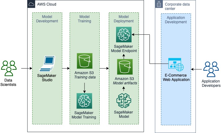
After the model is deployed into the production environment, your data scientists can use Amazon SageMaker Model Monitor to continuously monitor the quality of the ML models in real time. They can also set up an automated alert triggering system when deviations in the model quality occur, such as data drift and anomalies. Amazon CloudWatch Logs collects log files monitoring the model status and notifies you when the quality of the model reaches certain thresholds. This enables your data scientists to take corrective actions, such as retraining models, auditing upstream systems, or fixing quality issues without having to monitor models manually. With AWS Managed Services, your data science team can avoid the downside of implementing monitoring solutions from scratch.

Your data scientists can reduce the overall time required to deploy their ML models in production by automating load testing and model tuning across SageMaker ML instances by using Amazon SageMaker Inference Recommender. It helps your data scientists select the best instance type and configuration (such as instance count, container parameters, and model optimizations) for their ML models.

Lastly, it’s always a best practice to decouple hosting your ML model from hosting your application. In this approach, the data scientists use dedicated resources to host their ML model, specifically ones that are separated from the application, which greatly simplifies the process to push better models. This is a key step in the innovation flywheel. This also prevents any form of tight coupling between the hosted ML model and the application, thereby enabling the model to be highly performant.

In addition to improving the model performance with updated research trends, this approach provides the ability to redeploy a model with updated data. The global COVID-19 pandemic has demonstrated the reality that markets are changing all the time, and the ML model need to stay up to date with the latest trends. The only way you can deliver on that requirement is by being able to retrain and redeploy your model with updated data.

Conclusion

Check out the whitepaper Hybrid Machine Learning, in which we look at additional patterns for hosting ML models via Lambda@Edge, AWS Outposts, AWS Local Zones, and AWS Wavelength. We explore hybrid ML patterns across the entire ML lifecycle. We look at developing locally, while training and deploying in the cloud. We discuss patterns for training locally to deploy on the cloud, and even to host ML models in the cloud to serve applications on premises.

How are you integrating the cloud with your existing on-premises ML infrastructure? Please share your feedback about hybrid ML in the comments so we can continue to improve our products, features, and documentation. If you want to engage the authors of this document for advice on your cloud migration, contact us at hybrid-ml-support@amazon.com.


About the Authors

Alak Eswaradass is a Solutions Architect at AWS, based in Chicago, Illinois. She is passionate about helping customers design cloud architectures utilizing AWS services to solve business challenges. She hangs out with her daughters and explores the outdoors in her free time.

Emily Webber joined AWS just after SageMaker launched, and has been trying to tell the world about it ever since! Outside of building new ML experiences for customers, Emily enjoys meditating and studying Tibetan Buddhism.

Roop Bains is a Solutions Architect at AWS focusing on AI/ML. He is passionate about machine learning and helping customers achieve their business objectives. In his spare time, he enjoys reading and hiking.

Read More

Use deep learning frameworks natively in Amazon SageMaker Processing

Until recently, customers who wanted to use a deep learning (DL) framework with Amazon SageMaker Processing faced increased complexity compared to those using scikit-learn or Apache Spark. This post shows you how SageMaker Processing has simplified running machine learning (ML) preprocessing and postprocessing tasks with popular frameworks such as PyTorch, TensorFlow, Hugging Face, MXNet, and XGBoost.

Benefits of SageMaker Processing

Training an ML model takes many steps. One of them, data preparation, is paramount to creating an accurate ML model. A typical preprocessing step includes operations such as the following:

  • Converting the dataset to the input format expected by the ML algorithm that you’re using
  • Transforming existing features to a more expressive representation, such as one-hot encoding categorical features
  • Rescaling or normalizing numerical features
  • Engineering high-level features; for example, replacing mailing addresses with GPS coordinates
  • Cleaning and tokenizing text for natural language processing (NLP) applications
  • Resizing, centering, or augmenting images for computer vision applications

Likewise, you often need to run postprocessing jobs (for example, filtering or collating) and model evaluation jobs (scoring models against different test sets) as part of your ML model development lifecycle.

All these tasks involve running custom scripts on your dataset and saving the processed version for later use by your training jobs. In 2019, we launched SageMaker Processing, a capability of Amazon SageMaker that lets you run your preprocessing, postprocessing, and model evaluation workloads on a fully managed infrastructure. It does the heavy lifting for you, managing the infrastructure that runs your bespoke scripts. It spins up the necessary resources to do the job and tears them down when it’s done.

The SageMaker Python SDK provides a SageMaker Processing library that lets you do the following:

  • Use scikit-learn data processing features through a built-in container image provided by SageMaker with a scikit-learn framework. You can instantiate the SKLearnProcessor class provided in the SageMaker Python SDK and feed it your scikit-learn script.
  • Use Apache Spark for distributed data processing through a built-in Apache Spark container image provided by SageMaker. Similar to the previous process, you can instantiate the PySparkProcessor class provided in the SageMaker Python SDK and feed it your PySpark script.
  • Lastly, you can bring you own container to do the job. If you want preprocessing or postprocessing tasks to use libraries or frameworks other than scikit-learn and PySpark, you can package your custom code in a container. You then instantiate the ScriptProcessor class through your container image and feed it your data processing script.

Before release 2.52 of the SageMaker Python SDK, using SageMaker Processing in combination with popular ML frameworks such as PyTorch, TensorFlow, Hugging Face, MXNet, and XGBoost required you to bring your own container. You had to first build a container and then make sure that it included the relevant framework and all its dependencies. We wanted to simplify data scientists’ lives by removing the need to create a custom container image for these popular frameworks. And we wanted to deliver the same consistent experience people already had with Processing when using scikit-learn or Spark.

In the following sections, we show you how to natively use popular ML frameworks such as PyTorch, TensorFlow, Hugging Face, or MXNet with SageMaker Processing, without having to build a single container.

Using machine learning / deep learning frameworks in SageMaker Processing

The introduction of FrameworkProcessor—in release 2.52 of the SageMaker Python SDK in August 2021—changed everything. You can now use SageMaker Processing with your preferred ML framework among PyTorch, TensorFlow, Hugging Face, MXNet, and XGBoost. ML practitioners can now focus on perfecting their data processing code instead of spending additional energy on maintaining the lifecycle of custom containers. Now you can use one of the built-in containers and classes provided by SageMaker to use the data processing features of any of the previously mentioned frameworks. For this post, we only test one framework: PyTorch. However, you can reproduce the same procedures for any of the four other supported frameworks. The differences from one framework to the next are in the FrameworkProcessor subclass being used, the framework release, and the specifics of each framework for the data processing script.

The dataset

To illustrate our solution, let’s imagine that we plan to train a model to classify animal pictures. We rely on a publicly available dataset, the COCO dataset, which contains images from Flickr representing a real-world dataset not pre-formatted or resized specifically for deep learning. This makes it a good fit for our example scenario. Before we even get to the training stage, our initial problem is that the images we want to use to train our model come in all forms and shapes. Therefore, to make sure that this doesn’t affect our training or impact the quality of our model, we preprocess the images. In particular, we make sure that they’re the same shape and size before moving any further.

The COCO dataset provides an annotation file that contains information on each image in the dataset, such as the class, superclass, file name, and URL to download the file. We limit the scope of the dataset for the sake of this example by only using animal images. For the train and validation sets, the data we need for the image labels and the file paths are under different headings in the annotations. We only use a small fraction of the dataset, sufficient for this example.

Processing logic

Before we train our model, all image data must have the same dimensions for length, width, and channel. Typically, algorithms use a square format, with identical length and width. However, most real-world datasets such as ours contain images in many different dimensions and ratios. To prepare our dataset for training, we need to resize and crop the images if they aren’t already square.

We also randomly augment the images to help our training algorithm generalize better. We only augment the training data, not the validation or test data, because we want to generate a prediction on the image as it normally would be presented for inference.

Our processing stage consists of two steps.

First, we instantiate the PyTorchProcessor class needed to run our bespoke data processing script:

import boto3
import sagemaker
from sagemaker import get_execution_role
from sagemaker.pytorch.processing import PyTorchProcessor

region = boto3.session.Session().region_name

role = get_execution_role()
pytorch_processor = PyTorchProcessor(
    framework_version="1.8", 
    role=role, 
    instance_type="ml.m5.xlarge", 
    instance_count=1
)

Second, we need to pass it the instructions to conduct the actual data processing tasks that are contained in our script:

  • The dataset (coco-annotations.zip) is automatically copied inside the container under the destination directory (/opt/ml/processing/input). We could add additional inputs if needed.
  • This is where the Python script (preprocessing.py) reads it. By specifying source_dir, we instruct Processing where to find the script and any of its dependencies. For instance, in source_dir you can find an extra file (script_utils.py) used by our main script, and a file to make sure that all dependencies are satisfied (requirements.txt). We then also pass any command line arguments useful to our script.
  • Our preprocessing script then processes the data, splits it three ways, and saves the files inside the container under /opt/ml/processing/output/train, /opt/ml/processing/output/validation, and /opt/ml/processing/output/test. We added more output to illustrate the flexibility of saving any useful data that results from that processing step for further use.
  • When the job is complete, all outputs are automatically copied to your default SageMaker bucket in Amazon Simple Storage Service (Amazon S3).

We run this step with the following code:

from sagemaker.processing import ProcessingInput, ProcessingOutput

pytorch_processor.run(
    code="preprocessing.py",
    source_dir="scripts",
    arguments = ['Debug', 'Not used'],
    inputs=[ProcessingInput(source="coco-annotations.zip", destination="/opt/ml/processing/input")],
    outputs=[
        ProcessingOutput(source="/opt/ml/processing/tmp/data_structured", output_name="data_structured"),
        ProcessingOutput(source="/opt/ml/processing/output/train", output_name="train"),
        ProcessingOutput(source="/opt/ml/processing/output/val", output_name="validation"),
        ProcessingOutput(source="/opt/ml/processing/output/test", output_name="test"),
        ProcessingOutput(source="/opt/ml/processing/logs", output_name="logs"),
    ],
)

At the end of this processing step, after sampling our initial dataset, we restructure it to fit the actual structure expected by the major ML frameworks. We also center, crop, and augment the images. We’re ready to proceed to the next stage and train our model. We also add an extra output (the data_structured folder) to save the restructured source data. This allows us to reuse the same dataset for further processing or training without restarting the whole preparation from scratch (that is, from the annotations file). More details on this can be found in the script.

Conclusion

In this post, we showed you how SageMaker Processing has simplified the use of the most popular ML frameworks, such as PyTorch, TensorFlow, MXNet, Hugging Face, and XGBoost. This is possible thanks to the introduction of FrameworkProcessor in the recent releases (2.52+) of the SageMaker Python SDK. You can now use the existing SageMaker containers provided natively for these frameworks with SageMaker Processing, and focus solely on your data processing code. Behind the scenes, SageMaker Processing manages the necessary infrastructure for you.

We hope this gave you a glimpse into the possibilities offered by SageMaker Processing. As a next step, you can look beyond preprocessing and postprocessing steps and consider the full lifecycle of an ML model. SageMaker Processing can play an active role before the training takes place but also post-training for any postprocessing tasks. You may want to also look at SageMaker Pipelines to automate the entire model lifecycle by crafting all these different steps together into a model pipeline.

This post was inspired by the post Amazon SageMaker Processing – Fully Managed Data Processing and Model Evaluation when SageMaker Processing first launched. Check out the SageMaker Python SDK for more details on the other supported frameworks: Hugging Face, TensorFlow, MXNet, XGBoost.

Sample notebooks and scripts for all four supported frameworks are available on GitHub: PyTorch example, Hugging Face example, TensorFlow example, MXNet example.

If you have feedback about this post, let us know in the comments section. If you have questions about this post, start a new thread on one of the AWS Developer forums or contact AWS Support.


About the Authors

Patrick Sard works as a Solutions Architect at AWS in Brussels, Belgium. Apart from being a cloud enthusiast, Patrick loves practicing tai chi (preferably Chen style), enjoys an occasional wine-tasting (he trained as a sommelier), and is an avid tennis player.

Davide Gallitelli is a Specialist Solutions Architect for AI/ML in the EMEA region. He is based in Brussels and works closely with customers throughout Benelux. He has been a developer since he was very young, and started coding at the age of 7. He discovered AI/ML while at university, and has fallen in love with it since then.

Read More

Have a Holly, Jolly Gaming Season on GeForce NOW

Happy holidays, members.

This GFN Thursday is packed with winter sales for several games streaming on GeForce NOW, as well as seasonal in-game events. Plus, for those needing a last minute gift for a gamer in their lives, we’ve got you covered with digital gift cards for Priority memberships.

To top it all off, six new games join the GeForce NOW library this week for some festive fun.

Jingle Bells, Holiday Sales, Events Are on the Way

Whether you made the naughty or nice list this year, there are plenty of games on your wishlist on sale.

The Witcher 3: Wild Hunt GOTY on GeForce NOW
Save big on some of PC gaming’s best, including The Witcher 3: Wild Hunt GOTY.

Snag some top titles from Square Enix like Guardians of the Galaxy and Life is Strange: True Colors. Dive into great games from Deep Silver like Metro Exodus and Kingdom Come Deliverance. Experience hits from Ubisoft like Far Cry 6 and Assassin’s Creed Valhalla. Get your GOG game on playing Cyberpunk 2077 or The Witcher 3: Wild Hunt GOTY.

To catch even more of the games from the GeForce NOW library on sale this holiday season, check out the “Sales and Special Offers” row on the GeForce NOW app.

On top of these winter sales and for a limited time, get the gift of a copy of Crysis Remastered free with the purchase of a six-month Priority membership or the new GeForce NOW RTX 3080 membership. Terms and conditions apply.

World of Tanks streaming on GeForce NOW
Yes, this is really happening.

Also, keep an eye out for holiday-themed in-game events in World of Tanks and more. Get to the tank in the Schwarzenegger Campaign, where you will receive missions from Arnold himself.

With over 1,100 titles streaming on the cloud, including nearly 100 free-to-play options and more coming every week, there’s a game for everyone to enjoy this holiday.

The Perfect Gift for a Gamer

GeForce NOW Digital Gift Cards
The perfect digital stocking stuffer for your favorite gamer.

The perfect last-minute present for a gamer in your life is the gift of PC gaming on any device.

Grab a GeForce NOW Priority membership digital gift card, available in two-, six- or 12-month options. Power up your gamer’s GeForce NOW compatible devices with the kick of a full gaming rig, priority access to gaming servers, extended session lengths and RTX ON to take supported games to the next level of rendering quality.

Check out the GeForce NOW membership page for more information on priority benefits.

Gift cards can be redeemed on an existing GeForce NOW account or added to a new one. Existing Founders and Priority members will have the number of months added to their accounts.

Let it Stream, Let it Stream, Let it Stream

No matter if the weather outside is frightful, streaming games is delightful.

GFN Thursday is all about games. It also means taking games to the next level. This week, Far Cry 6 and Bright Memory: Infinite go bigger and bolder with support for RTX ON.

Farming Simulator 22 on GeForce NOW
Create your own farm and let the good times grow in Farming Simulator 22.

Plus, this GFN Thursday, enjoy six new games ready to stream from the GeForce NOW library:

Note: members who purchased the Farming Simulator 22 DLC directly from their website will not be able to access it on GeForce NOW. DLC purchased from the respective supported game store — Steam or Epic Games Store — will be playable.

We make every effort to launch games on GeForce NOW as close to their release as possible, but, in some instances, games may not be available immediately.

Also, keep an eye out for the free Epic Games Store titles that are being given away over the holidays. Like last year, we’ll look to add as many of these as we can when we return next year.

Whether you’re celebrating the holidays or just looking forward to a weekend full of gaming, tell us what games are bringing you joy on Twitter or in the comments below.

The post Have a Holly, Jolly Gaming Season on GeForce NOW appeared first on The Official NVIDIA Blog.

Read More

TorchVision has a new backwards compatible API for building models with multi-weight support. The new API allows loading different pre-trained weights on the same model variant, keeps track of vital meta-data such as the classification labels and includes the preprocessing transforms necessary for using the models. In this blog post, we plan to review the prototype API, show-case its features and highlight key differences with the existing one.

We are hoping to get your thoughts about the API prior finalizing it. To collect your feedback, we have created a Github issue where you can post your thoughts, questions and comments.

Limitations of the current API

TorchVision currently provides pre-trained models which could be a starting point for transfer learning or used as-is in Computer Vision applications. The typical way to instantiate a pre-trained model and make a prediction is:

import torch

from PIL import Image
from torchvision import models as M
from torchvision.transforms import transforms as T


img = Image.open("test/assets/encode_jpeg/grace_hopper_517x606.jpg")

# Step 1: Initialize model
model = M.resnet50(pretrained=True)
model.eval()

# Step 2: Define and initialize the inference transforms
preprocess = T.Compose([
    T.Resize([256, ]),
    T.CenterCrop(224),
    T.PILToTensor(),
    T.ConvertImageDtype(torch.float),
    T.Normalize([0.485, 0.456, 0.406], [0.229, 0.224, 0.225])
])

# Step 3: Apply inference preprocessing transforms
batch = preprocess(img).unsqueeze(0)
prediction = model(batch).squeeze(0).softmax(0)

# Step 4: Use the model and print the predicted category
class_id = prediction.argmax().item()
score = prediction[class_id].item()
with open("imagenet_classes.txt", "r") as f:
    categories = [s.strip() for s in f.readlines()]
    category_name = categories[class_id]
print(f"{category_name}: **** {100 * score}%")

There are a few limitations with the above approach:

  1. Inability to support multiple pre-trained weights: Since the pretrained variable is boolean, we can only offer one set of weights. This poses a severe limitation when we significantly improve the accuracy of existing models and we want to make those improvements available to the community. It also stops us from offering pre-trained weights of the same model variant on different datasets.
  2. Missing inference/preprocessing transforms: The user is forced to define the necessary transforms prior using the model. The inference transforms are usually linked to the training process and dataset used to estimate the weights. Any minor discrepancies in these transforms (such as interpolation value, resize/crop sizes etc) can lead to major reductions in accuracy or unusable models.
  3. Lack of meta-data: Critical pieces of information in relation to the weights are unavailable to the users. For example, one needs to look into external sources and the documentation to find things like the category labels, the training recipe, the accuracy metrics etc.

The new API addresses the above limitations and reduces the amount of boilerplate code needed for standard tasks.

Overview of the prototype API

Let’s see how we can achieve exactly the same results as above using the new API:

from PIL import Image
from torchvision.prototype import models as PM


img = Image.open("test/assets/encode_jpeg/grace_hopper_517x606.jpg")

# Step 1: Initialize model
weights = PM.ResNet50_Weights.ImageNet1K_V1
model = PM.resnet50(weights=weights)
model.eval()

# Step 2: Initialize the inference transforms
preprocess = weights.transforms()

# Step 3: Apply inference preprocessing transforms
batch = preprocess(img).unsqueeze(0)
prediction = model(batch).squeeze(0).softmax(0)

# Step 4: Use the model and print the predicted category
class_id = prediction.argmax().item()
score = prediction[class_id].item()
category_name = weights.meta["categories"][class_id]
print(f"{category_name}: **** {100 * score}**%**")

As we can see the new API eliminates the aforementioned limitations. Let’s explore the new features in detail.

Multi-weight support

At the heart of the new API, we have the ability to define multiple different weights for the same model variant. Each model building method (eg resnet50) has an associated Enum class (eg ResNet50_Weights) which has as many entries as the number of pre-trained weights available. Additionally, each Enum class has a default alias which points to the best available weights for the specific model. This allows the users who want to always use the best available weights to do so without modifying their code.

Here is an example of initializing models with different weights:

from torchvision.prototype.models import resnet50, ResNet50_Weights

# Legacy weights with accuracy 76.130%
model = resnet50(weights=ResNet50_Weights.ImageNet1K_V1)

# New weights with accuracy 80.674%
model = resnet50(weights=ResNet50_Weights.ImageNet1K_V2)

# Best available weights (currently alias for ImageNet1K_V2)
model = resnet50(weights=ResNet50_Weights.default)

# No weights - random initialization
model = resnet50(weights=None)

Associated meta-data & preprocessing transforms

The weights of each model are associated with meta-data. The type of information we store depends on the task of the model (Classification, Detection, Segmentation etc). Typical information includes a link to the training recipe, the interpolation mode, information such as the categories and validation metrics. These values are programmatically accessible via the meta attribute:

from torchvision.prototype.models import ResNet50_Weights

# Accessing a single record
size = ResNet50_Weights.ImageNet1K_V2.meta["size"]

# Iterating the items of the meta-data dictionary
for k, v in ResNet50_Weights.ImageNet1K_V2.meta.items():
    print(k, v)

Additionally, each weights entry is associated with the necessary preprocessing transforms. All current preprocessing transforms are JIT-scriptable and can be accessed via the transforms attribute. Prior using them with the data, the transforms need to be initialized/constructed. This lazy initialization scheme is done to ensure the solution is memory efficient. The input of the transforms can be either a PIL.Image or a Tensor read using torchvision.io.

from torchvision.prototype.models import ResNet50_Weights

# Initializing preprocessing at standard 224x224 resolution
preprocess = ResNet50_Weights.ImageNet1K.transforms()

# Initializing preprocessing at 400x400 resolution
preprocess = ResNet50_Weights.ImageNet1K.transforms(crop_size=400, resize_size=400)

# Once initialized the callable can accept the image data:
# img_preprocessed = preprocess(img)

Associating the weights with their meta-data and preprocessing will boost transparency, improve reproducibility and make it easier to document how a set of weights was produced.

Get weights by name

The ability to link directly the weights with their properties (meta data, preprocessing callables etc) is the reason why our implementation uses Enums instead of Strings. Nevertheless for cases when only the name of the weights is available, we offer a method capable of linking Weight names to their Enums:

from torchvision.prototype.models import get_weight

# Weights can be retrieved by name:
assert get_weight("ResNet50_Weights.ImageNet1K_V1") == ResNet50_Weights.ImageNet1K_V1
assert get_weight("ResNet50_Weights.ImageNet1K_V2") == ResNet50_Weights.ImageNet1K_V2

# Including using the default alias:
assert get_weight("ResNet50_Weights.default") == ResNet50_Weights.ImageNet1K_V2

Deprecations

In the new API the boolean pretrained and pretrained_backbone parameters, which were previously used to load weights to the full model or to its backbone, are deprecated. The current implementation is fully backwards compatible as it seamlessly maps the old parameters to the new ones. Using the old parameters to the new builders emits the following deprecation warnings:

>>> model = torchvision.prototype.models.resnet50(pretrained=True)
 UserWarning: The parameter 'pretrained' is deprecated, please use 'weights' instead.
UserWarning: 
Arguments other than a weight enum or `None` for 'weights' are deprecated. 
The current behavior is equivalent to passing `weights=ResNet50_Weights.ImageNet1K_V1`. 
You can also use `weights=ResNet50_Weights.default` to get the most up-to-date weights.

Additionally the builder methods require using keyword parameters. The use of positional parameter is deprecated and using them emits the following warning:

>>> model = torchvision.prototype.models.resnet50(None)
UserWarning: 
Using 'weights' as positional parameter(s) is deprecated. 
Please use keyword parameter(s) instead.

Testing the new API

Migrating to the new API is very straightforward. The following method calls between the 2 APIs are all equivalent:

# Using pretrained weights:
torchvision.prototype.models.resnet50(weights=ResNet50_Weights.ImageNet1K_V1)
torchvision.models.resnet50(pretrained=True)
torchvision.models.resnet50(True)

# Using no weights:
torchvision.prototype.models.resnet50(weights=None)
torchvision.models.resnet50(pretrained=False)
torchvision.models.resnet50(False)

Note that the prototype features are available only on the nightly versions of TorchVision, so to use it you need to install it as follows:

conda install torchvision -c pytorch-nightly

For alternative ways to install the nightly have a look on the PyTorch download page. You can also install TorchVision from source from the latest main; for more information have a look on our repo.

Accessing state-of-the-art model weights with the new API

If you are still unconvinced about giving a try to the new API, here is one more reason to do so. We’ve recently refreshed our training recipe and achieved SOTA accuracy from many of our models. The improved weights can easily be accessed via the new API. Here is a quick overview of the model improvements:
[Image: chart.png] |Model |Old Acc@1 |New Acc@1 |
|— |— |— |
|EfficientNet B1 |78.642 |79.838 |
|MobileNetV3 Large |74.042 |75.274 |
|Quantized ResNet50 |75.92 |80.282 |
|Quantized ResNeXt101 32x8d |78.986 |82.574 |
|RegNet X 400mf * |72.834 |74.864 |
|RegNet X 800mf * |75.212 |77.522 |
|RegNet X 1 6gf * |77.04 |79.668 |
|RegNet X 3 2gf * |78.364 |81.198 |
|RegNet X 8gf * |79.344 |81.682 |
|RegNet X 16gf * |80.058 |82.72 |
|RegNet X 32gf * |80.622 |83.018 |
|RegNet Y 400mf * |74.046 |75.806 |
|RegNet Y 800mf * |76.42 |78.838 |
|RegNet Y 1 6gf * |77.95 |80.882 |
|RegNet Y 3 2gf * |78.948 |81.984 |
|RegNet Y 8gf * |80.032 |82.828 |
|RegNet Y 16gf * |80.424 |82.89 |
|RegNet Y 32gf * |80.878 |83.366 |
|ResNet50 |76.13 |80.674 |
|ResNet101 |77.374 |81.886 |
|ResNet152 |78.312 |82.284 |
|ResNeXt50 32x4d |77.618 |81.198 |
|ResNeXt101 32x8d |79.312 |82.834 |
|Wide ResNet50 2 |78.468 |81.602 |
|Wide ResNet101 2 |78.848 |82.51 |

  • At the time of writing, the RegNet refresh work is in progress, see PR 5107.

Please spare a few minutes to provide your feedback on the new API, as this is crucial for graduating it from prototype and including it in the next release. You can do this on the dedicated Github Issue. We are looking forward to reading your comments!

Read More

Introducing TorchVision’s New Multi-Weight Support API

TorchVision has a new backwards compatible API for building models with multi-weight support. The new API allows loading different pre-trained weights on the same model variant, keeps track of vital meta-data such as the classification labels and includes the preprocessing transforms necessary for using the models. In this blog post, we plan to review the prototype API, show-case its features and highlight key differences with the existing one.

We are hoping to get your thoughts about the API prior finalizing it. To collect your feedback, we have created a Github issue where you can post your thoughts, questions and comments.

Limitations of the current API

TorchVision currently provides pre-trained models which could be a starting point for transfer learning or used as-is in Computer Vision applications. The typical way to instantiate a pre-trained model and make a prediction is:

import torch

from PIL import Image
from torchvision import models as M
from torchvision.transforms import transforms as T


img = Image.open("test/assets/encode_jpeg/grace_hopper_517x606.jpg")

# Step 1: Initialize model
model = M.resnet50(pretrained=True)
model.eval()

# Step 2: Define and initialize the inference transforms
preprocess = T.Compose([
    T.Resize([256, ]),
    T.CenterCrop(224),
    T.PILToTensor(),
    T.ConvertImageDtype(torch.float),
    T.Normalize([0.485, 0.456, 0.406], [0.229, 0.224, 0.225])
])

# Step 3: Apply inference preprocessing transforms
batch = preprocess(img).unsqueeze(0)
prediction = model(batch).squeeze(0).softmax(0)

# Step 4: Use the model and print the predicted category
class_id = prediction.argmax().item()
score = prediction[class_id].item()
with open("imagenet_classes.txt", "r") as f:
    categories = [s.strip() for s in f.readlines()]
    category_name = categories[class_id]
print(f"{category_name}: **** {100 * score}%")

There are a few limitations with the above approach:

  1. Inability to support multiple pre-trained weights: Since the pretrained variable is boolean, we can only offer one set of weights. This poses a severe limitation when we significantly improve the accuracy of existing models and we want to make those improvements available to the community. It also stops us from offering pre-trained weights of the same model variant on different datasets.
  2. Missing inference/preprocessing transforms: The user is forced to define the necessary transforms prior using the model. The inference transforms are usually linked to the training process and dataset used to estimate the weights. Any minor discrepancies in these transforms (such as interpolation value, resize/crop sizes etc) can lead to major reductions in accuracy or unusable models.
  3. Lack of meta-data: Critical pieces of information in relation to the weights are unavailable to the users. For example, one needs to look into external sources and the documentation to find things like the category labels, the training recipe, the accuracy metrics etc.

The new API addresses the above limitations and reduces the amount of boilerplate code needed for standard tasks.

Overview of the prototype API

Let’s see how we can achieve exactly the same results as above using the new API:

from PIL import Image
from torchvision.prototype import models as PM


img = Image.open("test/assets/encode_jpeg/grace_hopper_517x606.jpg")

# Step 1: Initialize model
weights = PM.ResNet50_Weights.ImageNet1K_V1
model = PM.resnet50(weights=weights)
model.eval()

# Step 2: Initialize the inference transforms
preprocess = weights.transforms()

# Step 3: Apply inference preprocessing transforms
batch = preprocess(img).unsqueeze(0)
prediction = model(batch).squeeze(0).softmax(0)

# Step 4: Use the model and print the predicted category
class_id = prediction.argmax().item()
score = prediction[class_id].item()
category_name = weights.meta["categories"][class_id]
print(f"{category_name}: **** {100 * score}**%**")

As we can see the new API eliminates the aforementioned limitations. Let’s explore the new features in detail.

Multi-weight support

At the heart of the new API, we have the ability to define multiple different weights for the same model variant. Each model building method (eg resnet50) has an associated Enum class (eg ResNet50_Weights) which has as many entries as the number of pre-trained weights available. Additionally, each Enum class has a default alias which points to the best available weights for the specific model. This allows the users who want to always use the best available weights to do so without modifying their code.

Here is an example of initializing models with different weights:

from torchvision.prototype.models import resnet50, ResNet50_Weights

# Legacy weights with accuracy 76.130%
model = resnet50(weights=ResNet50_Weights.ImageNet1K_V1)

# New weights with accuracy 80.674%
model = resnet50(weights=ResNet50_Weights.ImageNet1K_V2)

# Best available weights (currently alias for ImageNet1K_V2)
model = resnet50(weights=ResNet50_Weights.default)

# No weights - random initialization
model = resnet50(weights=None)

Associated meta-data & preprocessing transforms

The weights of each model are associated with meta-data. The type of information we store depends on the task of the model (Classification, Detection, Segmentation etc). Typical information includes a link to the training recipe, the interpolation mode, information such as the categories and validation metrics. These values are programmatically accessible via the meta attribute:

from torchvision.prototype.models import ResNet50_Weights

# Accessing a single record
size = ResNet50_Weights.ImageNet1K_V2.meta["size"]

# Iterating the items of the meta-data dictionary
for k, v in ResNet50_Weights.ImageNet1K_V2.meta.items():
    print(k, v)

Additionally, each weights entry is associated with the necessary preprocessing transforms. All current preprocessing transforms are JIT-scriptable and can be accessed via the transforms attribute. Prior using them with the data, the transforms need to be initialized/constructed. This lazy initialization scheme is done to ensure the solution is memory efficient. The input of the transforms can be either a PIL.Image or a Tensor read using torchvision.io.

from torchvision.prototype.models import ResNet50_Weights

# Initializing preprocessing at standard 224x224 resolution
preprocess = ResNet50_Weights.ImageNet1K.transforms()

# Initializing preprocessing at 400x400 resolution
preprocess = ResNet50_Weights.ImageNet1K.transforms(crop_size=400, resize_size=400)

# Once initialized the callable can accept the image data:
# img_preprocessed = preprocess(img)

Associating the weights with their meta-data and preprocessing will boost transparency, improve reproducibility and make it easier to document how a set of weights was produced.

Get weights by name

The ability to link directly the weights with their properties (meta data, preprocessing callables etc) is the reason why our implementation uses Enums instead of Strings. Nevertheless for cases when only the name of the weights is available, we offer a method capable of linking Weight names to their Enums:

from torchvision.prototype.models import get_weight

# Weights can be retrieved by name:
assert get_weight("ResNet50_Weights.ImageNet1K_V1") == ResNet50_Weights.ImageNet1K_V1
assert get_weight("ResNet50_Weights.ImageNet1K_V2") == ResNet50_Weights.ImageNet1K_V2

# Including using the default alias:
assert get_weight("ResNet50_Weights.default") == ResNet50_Weights.ImageNet1K_V2

Deprecations

In the new API the boolean pretrained and pretrained_backbone parameters, which were previously used to load weights to the full model or to its backbone, are deprecated. The current implementation is fully backwards compatible as it seamlessly maps the old parameters to the new ones. Using the old parameters to the new builders emits the following deprecation warnings:

>>> model = torchvision.prototype.models.resnet50(pretrained=True)
 UserWarning: The parameter 'pretrained' is deprecated, please use 'weights' instead.
UserWarning: 
Arguments other than a weight enum or `None` for 'weights' are deprecated. 
The current behavior is equivalent to passing `weights=ResNet50_Weights.ImageNet1K_V1`. 
You can also use `weights=ResNet50_Weights.default` to get the most up-to-date weights.

Additionally the builder methods require using keyword parameters. The use of positional parameter is deprecated and using them emits the following warning:

>>> model = torchvision.prototype.models.resnet50(None)
UserWarning: 
Using 'weights' as positional parameter(s) is deprecated. 
Please use keyword parameter(s) instead.

Testing the new API

Migrating to the new API is very straightforward. The following method calls between the 2 APIs are all equivalent:

# Using pretrained weights:
torchvision.prototype.models.resnet50(weights=ResNet50_Weights.ImageNet1K_V1)
torchvision.models.resnet50(pretrained=True)
torchvision.models.resnet50(True)

# Using no weights:
torchvision.prototype.models.resnet50(weights=None)
torchvision.models.resnet50(pretrained=False)
torchvision.models.resnet50(False)

Note that the prototype features are available only on the nightly versions of TorchVision, so to use it you need to install it as follows:

conda install torchvision -c pytorch-nightly

For alternative ways to install the nightly have a look on the PyTorch download page. You can also install TorchVision from source from the latest main; for more information have a look on our repo.

Accessing state-of-the-art model weights with the new API

If you are still unconvinced about giving a try to the new API, here is one more reason to do so. We’ve recently refreshed our training recipe and achieved SOTA accuracy from many of our models. The improved weights can easily be accessed via the new API. Here is a quick overview of the model improvements:
[Image: chart.png] |Model |Old Acc@1 |New Acc@1 |
|— |— |— |
|EfficientNet B1 |78.642 |79.838 |
|MobileNetV3 Large |74.042 |75.274 |
|Quantized ResNet50 |75.92 |80.282 |
|Quantized ResNeXt101 32x8d |78.986 |82.574 |
|RegNet X 400mf * |72.834 |74.864 |
|RegNet X 800mf * |75.212 |77.522 |
|RegNet X 1 6gf * |77.04 |79.668 |
|RegNet X 3 2gf * |78.364 |81.198 |
|RegNet X 8gf * |79.344 |81.682 |
|RegNet X 16gf * |80.058 |82.72 |
|RegNet X 32gf * |80.622 |83.018 |
|RegNet Y 400mf * |74.046 |75.806 |
|RegNet Y 800mf * |76.42 |78.838 |
|RegNet Y 1 6gf * |77.95 |80.882 |
|RegNet Y 3 2gf * |78.948 |81.984 |
|RegNet Y 8gf * |80.032 |82.828 |
|RegNet Y 16gf * |80.424 |82.89 |
|RegNet Y 32gf * |80.878 |83.366 |
|ResNet50 |76.13 |80.674 |
|ResNet101 |77.374 |81.886 |
|ResNet152 |78.312 |82.284 |
|ResNeXt50 32x4d |77.618 |81.198 |
|ResNeXt101 32x8d |79.312 |82.834 |
|Wide ResNet50 2 |78.468 |81.602 |
|Wide ResNet101 2 |78.848 |82.51 |

  • At the time of writing, the RegNet refresh work is in progress, see PR 5107.

Please spare a few minutes to provide your feedback on the new API, as this is crucial for graduating it from prototype and including it in the next release. You can do this on the dedicated Github Issue. We are looking forward to reading your comments!

Read More