Live call analytics for your contact center with Amazon language AI services
Your contact center connects your business to your community, enabling customers to order products, callers to request support, clients to make appointments, and much more. When calls go well, callers retain a positive image of your brand, and are likely to return and recommend you to others. And the converse, of course, is also true.
Naturally, you want to do what you can to ensure that your callers have a good experience. There are two aspects to this:
- Help supervisors assess the quality of your caller’s experiences in real time – For example, your supervisors need to know if initially unhappy callers become happier as the call progresses. And if not, why? What actions can be taken, before the call ends, to assist the agent to improve the customer experience for calls that aren’t going well?
- Help agents optimize the quality of your caller’s experiences – For example, can you deploy live call transcription? This removes the need for your agents to take notes during calls, freeing them to focus more attention on providing positive customer interactions.
Contact Lens for Amazon Connect provides real-time supervisor and agent assist features that could be just what you need, but you may not yet be using Amazon Connect. You need a solution that works with your existing contact center.
Amazon Machine Learning (ML) services like Amazon Transcribe and Amazon Comprehend provide feature-rich APIs that you can use to transcribe and extract insights from your contact center audio at scale. Although you could build your own custom call analytics solution using these services, that requires time and resources. In this post, we introduce our new sample solution for live call analytics.
Solution overview
Our new sample solution, Live Call Analytics (LCA), does most of the heavy lifting associated with providing an end-to-end solution that can plug into your contact center and provide the intelligent insights that you need.
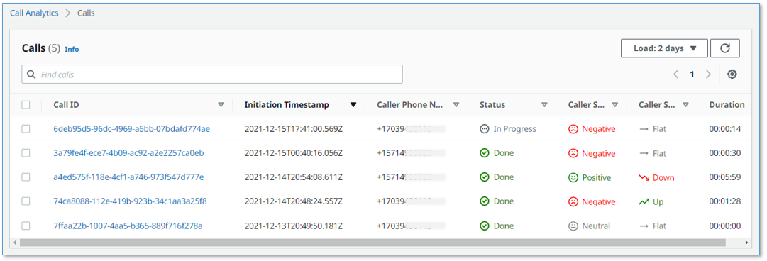
It has a call summary user interface, as shown in the following screenshot.
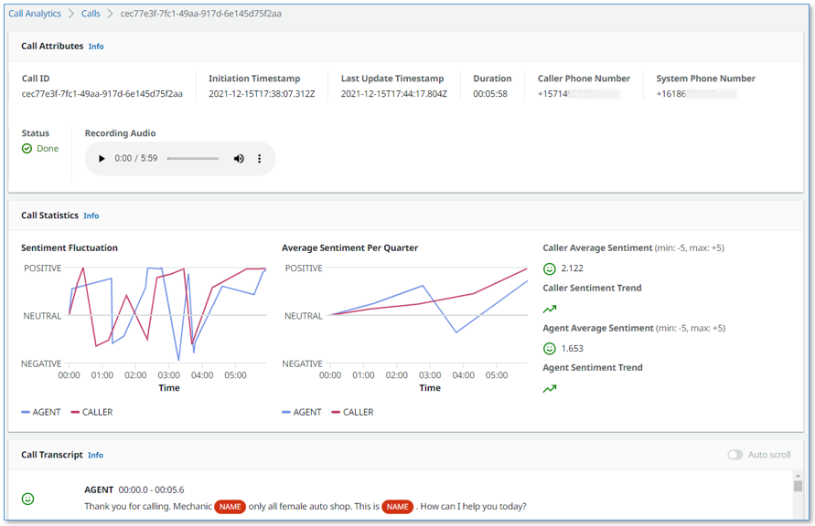
It also has a call detail user interface.
LCA currently supports the following features:
- Accurate streaming transcription with support for personally identifiable information (PII) redaction and custom vocabulary
- Sentiment detection
- Automatic scaling to handle call volume changes
- Call recording and archiving
- A dynamically updated web user interface for supervisors and agents:
- A call summary page that displays a list of in-progress and completed calls, with call timestamps, metadata, and summary statistics like duration, and sentiment trend
- Call detail pages showing live turn-by-turn transcription of the caller/agent dialog, turn-by-turn sentiment, and sentiment trend
- Standards-based telephony integration with your contact center using Session Recording Protocol (SIPREC)
- A built-in standalone demo mode that allows you to quickly install and try out LCA for yourself, without needing to integrate with your contact center telephony
- Easy-to-install resources with a single AWS CloudFormation template
This is just the beginning! We expect to add many more exciting features over time, based on your feedback.
Deploy the CloudFormation stack
Start your LCA experience by using AWS CloudFormation to deploy the sample solution with the built-in demo mode enabled.
The demo mode downloads, builds, and installs a small virtual PBX server on an Amazon Elastic Compute Cloud (Amazon EC2) instance in your AWS account (using the free open-source Asterisk project) so you can make test phone calls right away and see the solution in action. You can integrate it with your contact center later after evaluating the solution’s functionality for your unique use case.
- Use the appropriate Launch Stack button for the AWS Region in which you’ll use the solution. We expect to add support for additional Regions over time.
- US East (N. Virginia) us-east-1

- US West (Oregon) us-west-2
- US East (N. Virginia) us-east-1
- For Stack name, use the default value,
LiveCallAnalytics. - For Install Demo Asterisk Server, use the default value,
true. - For Allowed CIDR Block for Demo Softphone, use the IP address of your local computer with a network mask of
/32.
To find your computer’s IP address, you can use the website checkip.amazonaws.com.
Later, you can optionally install a softphone application on your computer, which you can register with LCA’s demo Asterisk server. This allows you to experiment with LCA using real two-way phone calls.
If that seems like too much hassle, don’t worry! Simply leave the default value for this parameter and elect not to register a softphone later. You will still be able to test the solution. When the demo Asterisk server doesn’t detect a registered softphone, it automatically simulates the agent side of the conversation using a built-in audio recording.
- For Allowed CIDR List for SIPREC Integration, leave the default value.
This parameter isn’t used for demo mode installation. Later, when you want to integrate LCA with your contact center audio stream, you use this parameter to specify the IP address of your SIPREC source hosts, such as your Session Border Controller (SBC) servers.
- For Authorized Account Email Domain, use the domain name part of your corporate email address (this allows others with email addresses in the same domain to sign up for access to the UI).
- For Call Audio Recordings Bucket Name, leave the value blank to have an Amazon Simple Storage Service (Amazon S3) bucket for your call recordings automatically created for you. Otherwise, use the name of an existing S3 bucket where you want your recordings to be stored.
- For all other parameters, use the default values.
If you want to customize the settings later, for example to apply PII redaction or custom vocabulary to improve accuracy, you can update the stack for these parameters.
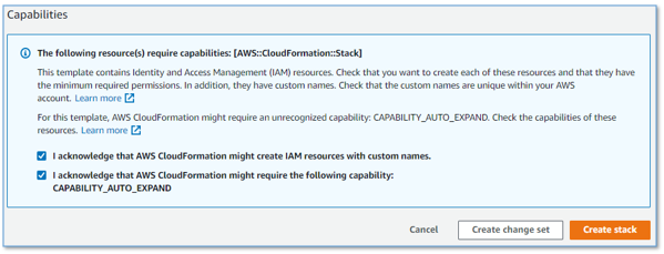
- Check the two acknowledgement boxes, and choose Create stack.

The main CloudFormation stack uses nested stacks to create the following resources in your AWS account:
- S3 buckets to hold build artifacts and call recordings
- An EC2 instance (t4g.large) with the demo Asterisk server installed, with VPC, security group, Elastic IP address, and internet gateway
- An Amazon Chime Voice Connector, configured to stream audio to Amazon Kinesis Video Streams
- An Amazon Elastic Container Service (Amazon ECS) instance that runs containers in AWS Fargate to relay streaming audio from Kinesis Video Streams to Amazon Transcribe and record transcription segments in Amazon DynamoDB, with VPC, NAT gateways, Elastic IP addresses, and internet gateway
- An AWS Lambda function to create and store final stereo call recordings
- A DynamoDB table to store call and transcription data, with Lambda stream processing that adds analytics to the live call data
- The AWS AppSync API, which provides a GraphQL endpoint to support queries and real-time updates
- Website components including S3 bucket, Amazon CloudFront distribution, and Amazon Cognito user pool
- Other miscellaneous supporting resources, including AWS Identity and Access Management (IAM) roles and policies (using least privilege best practices), Amazon Virtual Private Cloud (Amazon VPC) resources, Amazon EventBridge event rules, and Amazon CloudWatch log groups.
The stacks take about 20 minutes to deploy. The main stack status shows CREATE_COMPLETE when everything is deployed.

Create a user account
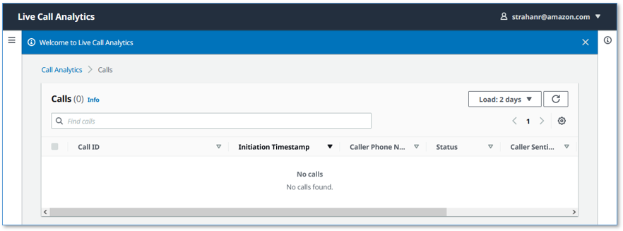
We now open the web user interface and create a user account.
- On the AWS CloudFormation console, choose the main stack,
LiveCallAnalytics, and choose the Outputs tab.
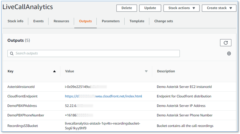
- Open your web browser to the URL shown as
CloudfrontEndpointin the outputs.
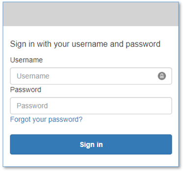
You’re directed to the login page.
- Choose Create account.

- For Username, use your email address that belongs to the email address domain you provided earlier.
- For Password, use a sequence that has a length of at least 8 characters, and contains uppercase and lowercase characters, plus numbers and special characters.
- Choose CREATE ACCOUNT.
The Confirm Sign up page appears.

Your confirmation code has been emailed to the email address you used as your username. Check your inbox for an email from no-reply@verificationemail.com with subject “Account Verification.”
- For Confirmation Code, copy and paste the code from the email.
- Choose CONFIRM.
You’re now logged in to LCA.
Make a test phone call
Call the number shown as DemoPBXPhoneNumber in the AWS CloudFormation outputs for the main LiveCallAnalytics stack.
You haven’t yet registered a softphone app, so the demo Asterisk server picks up the call and plays a recording. Listen to the recording, and answer the questions when prompted. Your call is streamed to the LCA application, and is recorded, transcribed, and analyzed. When you log in to the UI later, you can see a record of this call.
Optional: Install and register a softphone
If you want to use LCA with live two-person phone calls instead of the demo recording, you can register a softphone application with your new demo Asterisk server.
The following README has step-by-step instructions for downloading, installing, and registering a free (for non-commercial use) softphone on your local computer. The registration is successful only if Allowed CIDR Block for Demo Softphone correctly reflects your local machine’s IP address. If you got it wrong, or if your IP address has changed, you can choose the LiveCallAnalytics stack in AWS CloudFormation, and choose Update to provide a new value for Allowed CIDR Block for Demo Softphone.
If you still can’t successfully register your softphone, and you are connected to a VPN, disconnect and update Allowed CIDR Block for Demo Softphone—corporate VPNs can restrict IP voice traffic.
When your softphone is registered, call the phone number again. Now, instead of playing the default recording, the demo Asterisk server causes your softphone to ring. Answer the call on the softphone, and have a two-way conversation with yourself! Better yet, ask a friend to call your Asterisk phone number, so you can simulate a contact center call by role playing as caller and agent.
Explore live call analysis features
Now, with LCA successfully installed in demo mode, you’re ready to explore the call analysis features.
- Open the LCA web UI using the URL shown as
CloudfrontEndpointin the main stack outputs.
We suggest bookmarking this URL—you’ll use it often!
- Make a test phone call to the demo Asterisk server (as you did earlier).
- If you registered a softphone, it rings on your local computer. Answer the call, or better, have someone else answer it, and use the softphone to play the agent role in the conversation.
- If you didn’t register a softphone, the Asterisk server demo audio plays the role of agent.
Your phone call almost immediately shows up at the top of the call list on the UI, with the status In progress.
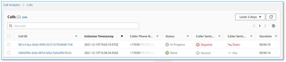
The call has the following details:
- Call ID – A unique identifier for this telephone call
- Initiation Timestamp – Shows the time the telephone call started
- Caller Phone Number – Shows the number of the phone from which you made the call
- Status – Indicates that the call is in progress
- Caller Sentiment – The average caller sentiment
- Caller Sentiment Trend –The caller sentiment trend
- Duration – The elapsed time since the start of the call
- Choose the call ID of your
In progresscall to open the live call detail page.

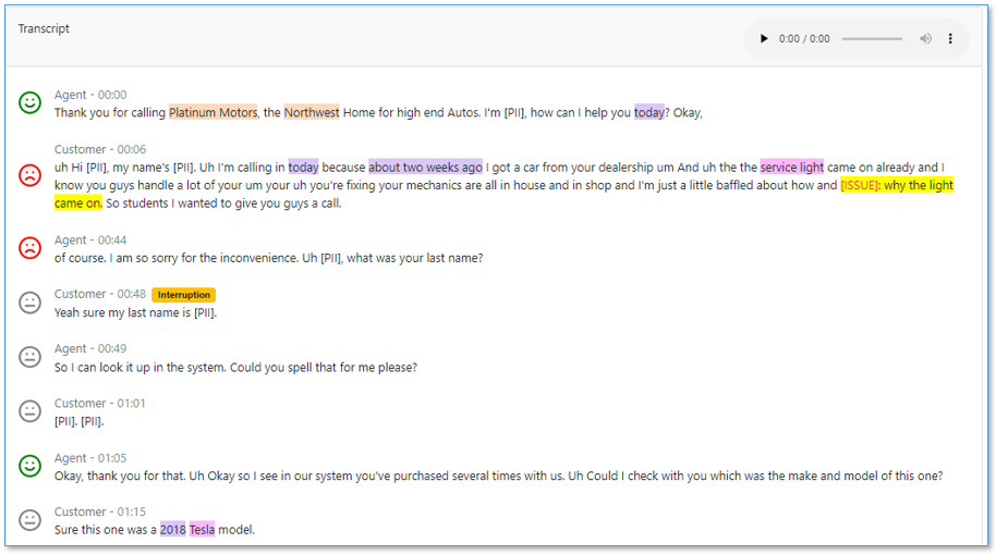
As you talk on the phone from which you made the call, your voice and the voice of the agent are transcribed in real time and displayed in the auto scrolling Call Transcript pane.
Each turn of the conversation (customer and agent) is annotated with a sentiment indicator. As the call continues, the sentiment for both caller and agent is aggregated over a rolling time window, so it’s easy to see if sentiment is trending in a positive or negative direction.
- End the call.
- Navigate back to the call list page by choosing Calls at the top of the page.
Your call is now displayed in the list with the status Done.
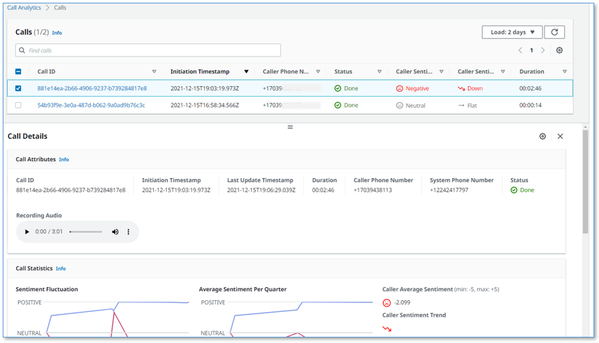
- To display call details for any call, choose the call ID to open the details page, or select the call to display the Calls list and Call Details pane on the same page.
You can change the orientation to a side-by-side layout using the Call Details settings tool (gear icon).
You can make a few more phone calls to become familiar with how the application works. With the softphone installed, ask someone else to call your Asterisk demo server phone number: pick up their call on your softphone and talk with them while watching the turn-by-turn transcription update in real time. Observe the low latency. Assess the accuracy of transcriptions and sentiment annotation—you’ll likely find that it’s not perfect, but it’s close! Transcriptions are less accurate when you use technical or domain-specific jargon, but you can use custom vocabulary to teach Amazon Transcribe new words and terms.
Processing flow overview
How did LCA transcribe and analyze your test phone calls? Let’s take a quick look at how it works.
The following diagram shows the main architectural components and how they fit together at a high level.

The demo Asterisk server is configured to use Voice Connector, which provides the phone number and SIP trunking needed to route inbound and outbound calls. When you configure LCA to integrate with your contact center instead of the demo Asterisk server, Voice Connector is configured to integrate instead with your existing contact center using SIP-based media recording (SIPREC) or network-based recording (NBR). In both cases, Voice Connector streams audio to Kinesis Video Streams using two streams per call, one for the caller and one for the agent.
When a new video stream is initiated, an event is fired using EventBridge. This event triggers a Lambda function, which uses an Amazon Simple Queue Service (Amazon SQS) queue to initiate a new call processing job in Fargate, a serverless compute service for containers. A single container instance processes multiple calls simultaneously. AWS auto scaling provisions and de-provisions additional containers dynamically as needed to handle changing call volumes.
The Fargate container immediately creates a streaming connection with Amazon Transcribe and starts consuming and relaying audio fragments from Kinesis Video Streams to Amazon Transcribe.
The container writes the streaming transcription results in real time to a DynamoDB table.
A Lambda function, the Call Event Stream Processor, fed by DynamoDB streams, processes and enriches call metadata and transcription segments. The event processor function interfaces with AWS AppSync to persist changes (mutations) in DynamoDB and to send real-time updates to logged in web clients.
The LCA web UI assets are hosted on Amazon S3 and served via CloudFront. Authentication is provided by Amazon Cognito. In demo mode, user identities are configured in an Amazon Cognito user pool. In a production setting, you would likely configure Amazon Cognito to integrate with your existing identity provider (IdP) so authorized users can log in with their corporate credentials.
When the user is authenticated, the web application establishes a secure GraphQL connection to the AWS AppSync API, and subscribes to receive real-time events such as new calls and call status changes for the calls list page, and new or updated transcription segments and computed analytics for the call details page.
The entire processing flow, from ingested speech to live webpage updates, is event driven, and so the end-to-end latency is small—typically just a few seconds.
Monitoring and troubleshooting
AWS CloudFormation reports deployment failures and causes on the relevant stack Events tab. See Troubleshooting CloudFormation for help with common deployment problems. Look out for deployment failures caused by limit exceeded errors; the LCA stacks create resources such as NAT gateways, Elastic IP addresses, and other resources that are subject to default account and Region Service Quotas.
Amazon Transcribe has a default limit of 25 concurrent transcription streams, which limits LCA to 12 concurrent calls (two streams per call). Request an increase for the number of concurrent HTTP/2 streams for streaming transcription if you need to handle a larger number of concurrent calls.
LCA provides runtime monitoring and logs for each component using CloudWatch:
-
Call trigger Lambda function – On the Lambda console, open the
LiveCallAnalytics-AISTACK-transcribingFargateXXXfunction. Choose the Monitor tab to see function metrics. Choose View logs in CloudWatch to inspect function logs. -
Call processing Fargate task – On the Amazon ECS console, choose the
LiveCallAnalyticscluster. Open theLiveCallAnalyticsservice to see container health metrics. Choose the Logs tab to inspect container logs. -
Call Event Stream Processor Lambda function – On the Lambda console, open the
LiveCallAnalytics-AISTACK-CallEventStreamXXXfunction. Choose the Monitor tab to see function metrics. Choose View logs in CloudWatch to inspect function logs. -
AWS AppSync API – On the AWS AppSync console, open the
CallAnalytics-LiveCallAnalytics-XXXAPI. Choose Monitoring in the navigation pane to see API metrics. Choose View logs in CloudWatch to inspect AppSyncAPI logs.
Cost assessment
This solution has hourly cost components and usage cost components.
The hourly costs add up to about $0.15 per hour, or $0.22 per hour with the demo Asterisk server enabled. For more information about the services that incur an hourly cost, see AWS Fargate Pricing, Amazon VPC pricing (for the NAT gateway), and Amazon EC2 pricing (for the demo Asterisk server).
The hourly cost components comprise the following:
- Fargate container – 2vCPU at $0.08/hour and 4 GB memory at $0.02/hour = $0.10/hour
- NAT gateways – Two at $0.09/hour
- EC2 instance – t4g.large at $0.07/hour (for demo Asterisk server)
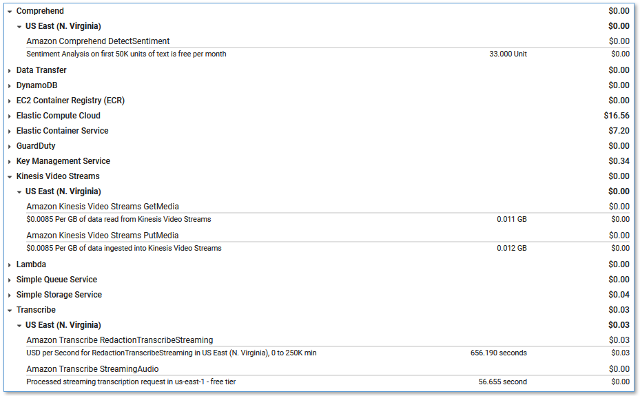
The usage costs add up to about $0.30 for a 5-minute call, although this can vary based on total usage, because usage affects Free Tier eligibility and volume tiered pricing for many services. For more information about the services that incur usage costs, see the following:
- AWS AppSync pricing
- Amazon Cognito Pricing
- Amazon Comprehend Pricing
- Amazon DynamoDB pricing
- Amazon EventBridge pricing
- Amazon Kinesis Video Streams pricing
- AWS Lambda Pricing
- Amazon SQS pricing
- Amazon S3 pricing
- Amazon Transcribe Pricing
- Amazon Voice Connector Chime pricing (streaming)
To explore LCA costs for yourself, use AWS Cost Explorer or choose Bill Details on the AWS Billing Dashboard to see your month-to-date spend by service.
Integrate with your contact center
To deploy LCA to analyze real calls to your contact center using AWS CloudFormation, update the existing LiveCallAnalytics demo stack, changing the parameters to disable demo mode.
Alternatively, delete the existing LiveCallAnalytics demo stack, and deploy a new LiveCallAnalytics stack (use the stack options from the previous section).
You could also deploy a new LiveCallAnalytics stack in a different AWS account or Region.
Use these parameters to configure LCA for contact center integration:
- For Install Demo Asterisk Server, enter
false. - For Allowed CIDR Block for Demo Softphone, leave the default value.
- For Allowed CIDR List for Siprec Integration, use the CIDR blocks of your SIPREC source hosts, such as your SBC servers. Use commas to separate CIDR blocks if you enter more than one.
When you deploy LCA, a Voice Connector is created for you. Use the Voice Connector documentation as guidance to configure this Voice Connector and your PBX/SBC for SIP-based media recording (SIPREC) or network-based recording (NBR). The Voice Connector Resources page provides some vendor-specific example configuration guides, including:
- SIPREC Configuration Guide: Cisco Unified Communications Manager (CUCM) and Cisco Unified Border Element (CUBE)
- SIPREC Configuration Guide: Avaya Aura Communication Manager and Session Manager with Sonus SBC 521
The LCA GitHub repository has additional vendor specific notes that you may find helpful; see SIPREC.md.
Customize your deployment
Use the following CloudFormation template parameters when creating or updating your stack to customize your LCA deployment:
- To use your own S3 bucket for call recordings, use Call Audio Recordings Bucket Name and Audio File Prefix.
- To redact PII from the transcriptions, set IsContentRedactionEnabled to
true. For more information, see Redacting or identifying PII in a real-time stream. - To improve transcription accuracy for technical and domain-specific acronyms and jargon, set UseCustomVocabulary to the name of a custom vocabulary that you already created in Amazon Transcribe. For more information, see Custom vocabularies.
LCA is an open-source project. You can fork the LCA GitHub repository, enhance the code, and send us pull requests so we can incorporate and share your improvements!
Clean up
When you’re finished experimenting with this solution, clean up your resources by opening the AWS CloudFormation console and deleting the LiveCallAnalytics stacks that you deployed. This deletes resources that were created by deploying the solution. The recording S3 buckets, DynamoDB table, and CloudWatch Log groups are retained after the stack is deleted to avoid deleting your data.
Post Call Analytics: Companion solution
Our companion solution, Post Call Analytics (PCA), offers additional insights and analytics capabilities by using the Amazon Transcribe Call Analytics batch API to detect common issues, interruptions, silences, speaker loudness, call categories, and more. Unlike LCA, which transcribes and analyzes streaming audio in real time, PCA transcribes and analyzes your call recordings after the call has ended. Configure LCA to store call recordings to the PCA’s ingestion S3 bucket, and use the two solutions together to get the best of both worlds. For more information, see Post call analytics for your contact center with Amazon language AI services.
Conclusion
The Live Call Analytics (LCA) sample solution offers a scalable, cost-effective approach to provide live call analysis with features to assist supervisors and agents to improve focus on your callers’ experience. It uses Amazon ML services like Amazon Transcribe and Amazon Comprehend to transcribe and extract real-time insights from your contact center audio.
The sample LCA application is provided as open source—use it as a starting point for your own solution, and help us make it better by contributing back fixes and features via GitHub pull requests. For expert assistance, AWS Professional Services and other AWS Partners are here to help.
We’d love to hear from you. Let us know what you think in the comments section, or use the issues forum in the LCA GitHub repository.
About the Authors
 Bob Strahan is a Principal Solutions Architect in the AWS Language AI Services team.
 Oliver Atoa is a Principal Solutions Architect in the AWS Language AI Services team.
 Sagar Khasnis is a Senior Solutions Architect focused on building applications for Productivity Applications. He is passionate about building innovative solutions using AWS services to help customers achieve their business objectives. In his free time, you can find him reading biographies, hiking, working out at a fitness studio, and geeking out on his personal rig at home.
 Court Schuett is a Chime Specialist SA with a background in telephony and now likes to build things that build things.
Post call analytics for your contact center with Amazon language AI services
Your contact center connects your business to your community, enabling customers to order products, callers to request support, clients to make appointments, and much more. Each conversation with a caller is an opportunity to learn more about that caller’s needs, and how well those needs were addressed during the call. You can uncover insights from these conversations that help you manage script compliance and find new opportunities to satisfy your customers, perhaps by expanding your services to address reported gaps, improving the quality of reported problem areas, or by elevating the customer experience delivered by your contact center agents.
Contact Lens for Amazon Connect provides call transcriptions with rich analytics capabilities that can provide these kinds of insights, but you may not currently be using Amazon Connect. You need a solution that works with your existing contact center call recordings.
Amazon Machine Learning (ML) services like Amazon Transcribe Call Analytics and Amazon Comprehend provide feature-rich APIs that you can use to transcribe and extract insights from your contact center audio recordings at scale. Although you could build your own custom call analytics solution using these services, that requires time and resources. In this post, we introduce our new sample solution for post call analytics.
Solution overview
Our new sample solution, Post Call Analytics (PCA), does most of the heavy lifting associated with providing an end-to-end solution that can process call recordings from your existing contact center. PCA provides actionable insights to spot emerging trends, identify agent coaching opportunities, and assess the general sentiment of calls.
You provide your call recordings, and PCA automatically processes them using Transcribe Call Analytics and other AWS services to extract valuable intelligence such as customer and agent sentiment, call drivers, entities discussed, and conversation characteristics such as non-talk time, interruptions, loudness, and talk speed. Transcribe Call Analytics detects issues using built-in ML models that have been trained using thousands of hours of conversations. With the automated call categorization capability, you can also tag conversations based on keywords or phrases, sentiment, and non-talk time. And you can optionally redact sensitive customer data such as names, addresses, credit card numbers, and social security numbers from both transcript and audio files.
PCA’s web user interface has a home page showing all your calls, as shown in the following screenshot.

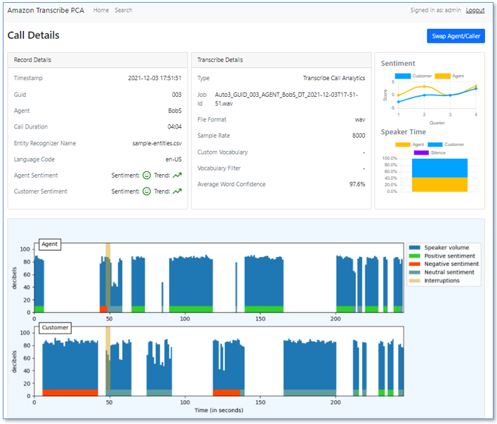
You can choose a record to see the details of the call, such as speech characteristics.
You can also scroll down to see annotated turn-by-turn call details.

You can search for calls based on dates, entities, or sentiment characteristics.

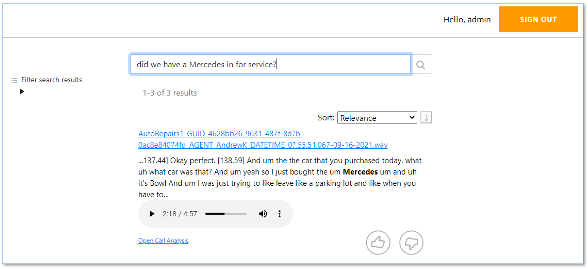
You can also search your call transcriptions.
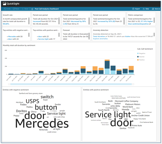
Lastly, you can query detailed call analytics data from your preferred business intelligence (BI) tool.
PCA currently supports the following features:
-
Transcription
- Batch turn-by-turn transcription with support for Amazon Transcribe custom vocabulary for accuracy of domain-specific terminology
- Personally identifiable information (PII) redaction from transcripts and audio files, and vocabulary filtering for masking custom words and phrases
- Multiple languages and automatic language detection
- Standard audio file formats
- Caller and agent speaker labels using channel identification or speaker diarization
-
Analytics
- Caller and agent sentiment details and trends
- Talk and non-talk time for both caller and agent
- Configurable Transcribe Call Analytics categories based on the presence or absence of keywords or phrases, sentiment, and non-talk time
- Detects callers’ main issues using built-in ML models in Transcribe Call Analytics
- Discovers entities referenced in the call using Amazon Comprehend standard or custom entity detection models, or simple configurable string matching
- Detects when caller and agent interrupt each other
- Speaker loudness
-
Search
- Search on call attributes such as time range, sentiment, or entities
- Search transcriptions
-
Other
- Detects metadata from audio file names, such as call GUID, agent’s name, and call date time
- Scales automatically to handle variable call volumes
- Bulk loads large archives of older recordings while maintaining capacity to process new recordings as they arrive
- Sample recordings so you can quickly try out PCA for yourself
- It’s easy to install with a single AWS CloudFormation template
This is just the beginning! We expect to add many more exciting features over time, based on your feedback.
Deploy the CloudFormation stack
Start your PCA experience by using AWS CloudFormation to deploy the solution with sample recordings loaded.
- Use the following Launch Stack button to deploy the PCA solution in the
us-east-1(N. Virginia) AWS Region.
The source code is available in our GitHub repository. Follow the directions in the README to deploy PCA to additional Regions supported by Amazon Transcribe.
- For Stack name, use the default value,
PostCallAnalytics. - For AdminUsername, use the default value, admin.
- For AdminEmail, use a valid email address—your temporary password is emailed to this address during the deployment.
- For loadSampleAudioFiles, change the value to
true. - For EnableTranscriptKendraSearch, change the value to
Yes, create new Kendra Index (Developer Edition).
If you have previously used your Amazon Kendra Free Tier allowance, you incur an hourly cost for this index (more information on cost later in this post). Amazon Kendra transcript search is an optional feature, so if you don’t need it and are concerned about cost, use the default value of No.
- For all other parameters, use the default values.
If you want to customize the settings later, for example to apply custom vocabulary to improve accuracy, or to customize entity detection, you can update the stack to set these parameters.
- Select the two acknowledgement boxes, and choose Create stack.
The main CloudFormation stack uses nested stacks to create the following resources in your AWS account:
- Amazon Simple Storage Service (Amazon S3) buckets to hold build artifacts and call recordings
- AWS Systems Manager Parameter Store settings to store configuration settings
- AWS Step Functions workflows to orchestrate recording file processing
- AWS Lambda functions to process audio files and turn-by-turn transcriptions and analytics
- Amazon DynamoDB tables to store call metadata
- Website components including S3 bucket, Amazon CloudFront distribution, and Amazon Cognito user pool
- Other miscellaneous supporting resources, including AWS Identity and Access Management (IAM) roles and policies (using least privilege best practices), Amazon Simple Queue Service (Amazon SQS) message queues, and Amazon CloudWatch log groups.
- Optionally, an Amazon Kendra index and AWS Amplify search application to provide intelligent call transcript search.
The stacks take about 20 minutes to deploy. The main stack status shows as CREATE_COMPLETE when everything is deployed.

Set your password
After you deploy the stack, you need to open the PCA web user interface and set your password.
- On the AWS CloudFormation console, choose the main stack,
PostCallAnalytics, and choose the Outputs tab.

- Open your web browser to the URL shown as
WebAppURLin the outputs.
You’re redirected to a login page.
- Open the email your received, at the email address you provided, with the subject “Welcome to the Amazon Transcribe Post Call Analytics (PCA) Solution!”
This email contains a generated temporary password that you can use to log in (as user admin) and create your own password.
- Set a new password.
Your new password must have a length of at least eight characters, and contain uppercase and lowercase characters, plus numbers and special characters.
You’re now logged in to PCA. Because you set loadSampleAudioFiles to true, your PCA deployment now has three sample calls pre-loaded for you to explore.
Optional: Open the transcription search web UI and set your permanent password
Follow these additional steps to log in to the companion transcript search web app, which is deployed only when you set EnableTranscriptKendraSearch when you launch the stack.
- On the AWS CloudFormation console, choose the main stack,
PostCallAnalytics, and choose the Outputs tab. - Open your web browser to the URL shown as
TranscriptionMediaSearchFinderURLin the outputs.
You’re redirected to the login page.

- Open the email your received, at the email address you provided, with the subject “Welcome to Finder Web App.”
This email contains a generated temporary password that you can use to log in (as user admin).
- Create your own password, just like you already did for the PCA web application.
As before, your new password must have a length of at least eight characters, and contain uppercase and lowercase characters, plus numbers and special characters.
You’re now logged in to the transcript search Finder application. The sample audio files are indexed already, and ready for search.
Explore post call analytics features
Now, with PCA successfully installed, you’re ready to explore the call analysis features.
Home page
To explore the home page, open the PCA web UI using the URL shown as WebAppURL in the main stack outputs (bookmark this URL, you’ll use it often!)
You already have three calls listed on the home page, sorted in descending time order (most recent first). These are the sample audio files.

The calls have the following key details:
- Job Name – Is assigned from the recording audio file name, and serves as a unique job name for this call
- Timestamp – Is parsed from the audio file name if possible, otherwise it’s assigned the time when the recording is processed by PCA
- Customer Sentiment and Customer Sentiment Trend – Show the overall caller sentiment and, importantly, whether the caller was more positive at the end of the call than at the beginning
- Language Code – Shows the specified language or the automatically detected dominant language of the call
Call details
Choose the most recently received call to open and explore the call detail page. You can review the call information and analytics such as sentiment, talk time, interruptions, and loudness.

Scroll down to see the following details:
- Entities grouped by entity type. Entities are detected by Amazon Comprehend and the sample entity recognizer string map.
- Categories detected by Transcribe Call Analytics. By default, there are no categories; see Call categorization for more information.
- Issues detected by the Transcribe Call Analytics built-in ML model. Issues succinctly capture the main reasons for the call. For more information, see Issue detection.

Scroll further to see the turn-by-turn transcription for the call, with annotations for speaker, time marker, sentiment, interruptions, issues, and entities.
Use the embedded media player to play the call audio from any point in the conversation. Set the position by choosing the time marker annotation on the transcript or by using the player time control. The audio player remains visible as you scroll down the page.
PII is redacted from both transcript and audio—redaction is enabled using the CloudFormation stack parameters.
Search based on call attributes
To try PCA’s built-in search, choose Search at the top of the screen. Under Sentiment, choose Average, Customer, and Negative to select the calls that had average negative customer sentiment.

Choose Clear to try a different filter. For Entities, enter Hyundai and then choose Search. Select the call from the search results and verify from the transcript that the customer was indeed calling about their Hyundai.
Search call transcripts
Transcript search is an experimental, optional, add-on feature powered by Amazon Kendra.
Open the transcript web UI using the URL shown as TranscriptionMediaSearchFinderURL in the main stack outputs. To find a recent call, enter the search query customer hit the wall.

The results show transcription extracts from relevant calls. Use the embedded audio player to play the associated section of the call recording.
You can expand Filter search results to refine the search results with additional filters. Choose Open Call Analytics to open the PCA call detail page for this call.
Query call analytics using SQL
You can integrate PCA call analytics data into a reporting or BI tool such as Amazon QuickSight by using Amazon Athena SQL queries. To try it, open the Athena query editor. For Database, choose pca.
Observe the table parsedresults. This table contains all the turn-by-turn transcriptions and analysis for each call, using nested structures.
You can also review flattened result sets, which are simpler to integrate into your reporting or analytics application. Use the query editor to preview the data.

Processing flow overview
How did PCA transcribe and analyze your phone call recordings? Let’s take a quick look at how it works.
The following diagram shows the main data processing components and how they fit together at a high level.

Call recording audio files are uploaded to the S3 bucket and folder, identified in the main stack outputs as InputBucket and InputBucketPrefix, respectively. The sample call recordings are automatically uploaded because you set the parameter loadSampleAudioFiles to true when you deployed PCA.
As each recording file is added to the input bucket, an S3 Event Notification triggers a Lambda function that initiates a workflow in Step Functions to process the file. The workflow orchestrates the steps to start an Amazon Transcribe batch job and process the results by doing entity detection and additional preparation of the call analytics results. Processed results are stored as JSON files in another S3 bucket and folder, identified in the main stack outputs as OutputBucket and OutputBucketPrefix.
As the Step Functions workflow creates each JSON results file in the output bucket, an S3 Event Notification triggers a Lambda function, which loads selected call metadata into a DynamoDB table.
The PCA UI web app queries the DynamoDB table to retrieve the list of processed calls to display on the home page. The call detail page reads additional detailed transcription and analytics from the JSON results file for the selected call.
Amazon S3 Lifecycle policies delete recordings and JSON files from both input and output buckets after a configurable retention period, defined by the deployment parameter RetentionDays. S3 Event Notifications and Lambda functions keep the DynamoDB table synchronized as files are both created and deleted.
When the EnableTranscriptKendraSearch parameter is true, the Step Functions workflow also adds time markers and metadata attributes to the transcription, which are loaded into an Amazon Kendra index. The transcription search web application is used to search call transcriptions. For more information on how this works, see Make your audio and video files searchable using Amazon Transcribe and Amazon Kendra.
Monitoring and troubleshooting
AWS CloudFormation reports deployment failures and causes on the stack Events tab. See Troubleshooting CloudFormation for help with common deployment problems.
PCA provides runtime monitoring and logs for each component using CloudWatch:
-
Step Functions workflow – On the Step Functions console, open the workflow
PostCallAnalyticsWorkflow. The Executions tab show the status of each workflow run. Choose any run to see details. Choose CloudWatch Logs from the Execution event history to examine logs for any Lambda function that was invoked by the workflow. -
PCA server and UI Lambda functions – On the Lambda console, filter by
PostCallAnalyticsto see all the PCA-related Lambda functions. Choose your function, and choose the Monitor tab to see function metrics. Choose View logs in CloudWatch to inspect function logs.
Cost assessment
For pricing information for the main services used by PCA, see the following:
- Amazon CloudFront Pricing
- Amazon CloudWatch pricing
- Amazon Cognito Pricing
- Amazon Comprehend Pricing
- Amazon DynamoDB pricing
- Amazon API Gateway pricing
- Amazon Kendra pricing (for the optional transcription search feature)
- AWS Lambda Pricing
- Amazon Transcribe Pricing
- Amazon S3 pricing
- AWS Step Functions Pricing
When transcription search is enabled, you incur an hourly cost for the Amazon Kendra index: $1.125/hour for the Developer Edition (first 750 hours are free), or $1.40/hour for the Enterprise Edition (recommended for production workloads).
All other PCA costs are incurred based on usage, and are Free Tier eligible. After the Free Tier allowance is consumed, usage costs add up to about $0.15 for a 5-minute call recording.
To explore PCA costs for yourself, use AWS Cost Explorer or choose Bill Details on the AWS Billing Dashboard to see your month-to-date spend by service.

Integrate with your contact center
You can configure your contact center to enable call recording. If possible, configure recordings for two channels (stereo), with customer audio on one channel (for example, channel 0) and the agent audio on the other channel (channel 1).
Via the AWS Command Line Interface (AWS CLI) or SDK, copy your contact center recording files to the PCA input bucket folder, identified in the main stack outputs as InputBucket and InputBucketPrefix. Alternatively, if you already save your call recordings to Amazon S3, use deployment parameters InputBucketName and InputBucketRawAudio to configure PCA to use your existing S3 bucket and prefix, so you don’t have to copy the files again.
Customize your deployment
Use the following CloudFormation template parameters when creating or updating your stack to customize your PCA deployment:
- To enable or disable the optional (experimental) transcription search feature, use
EnableTranscriptKendraSearch. - To use your existing S3 bucket for incoming call recordings, use
InputBucketandInputBucketPrefix. - To configure automatic deletion of recordings and call analysis data when using auto-provisioned S3 input and output buckets, use
RetentionDays. - To detect call timestamp, agent name, or call identifier (GUID) from the recording file name, use
FilenameDatetimeRegex,FilenameDatetimeFieldMap,FilenameGUIDRegex, andFilenameAgentRegex. - To use the standard Amazon Transcribe API instead of the default call analytics API, use TranscribeApiMode. PCA automatically reverts to the standard mode API for audio recordings that aren’t compatible with the call analytics API (for example, mono channel recordings). When using the standard API some call analytics, metrics such as issue detection and speaker loudness aren’t available.
- To set the list of supported audio languages, use
TranscribeLanguages. - To mask unwanted words, use
VocabFilterModeand setVocabFilterNameto the name of a vocabulary filter that you already created in Amazon Transcribe. See Vocabulary filtering for more information. - To improve transcription accuracy for technical and domain specific acronyms and jargon, set
VocabularyNameto the name of a custom vocabulary that you already created in Amazon Transcribe. See Custom vocabularies for more information. - To configure PCA to use single-channel audio by default, and to identify speakers using speaker diarizaton rather than channel identification, use
SpeakerSeparationTypeandMaxSpeakers. The default is to use channel identification with stereo files using Transcribe Call Analytics APIs to generate the richest analytics and most accurate speaker labeling. - To redact PII from the transcriptions or from the audio, set
CallRedactionTranscriptorCallRedactionAudioto true. See Redaction for more information. - To customize entity detection using Amazon Comprehend, or to provide your own CSV file to define entities, use the Entity detection parameters.
See the README on GitHub for more details on configuration options and operations for PCA.
PCA is an open-source project. You can fork the PCA GitHub repository, enhance the code, and send us pull requests so we can incorporate and share your improvements!
Clean up
When you’re finished experimenting with this solution, clean up your resources by opening the AWS CloudFormation console and deleting the PostCallAnalytics stacks that you deployed. This deletes resources that you created by deploying the solution. S3 buckets containing your audio recordings and analytics, and CloudWatch log groups are retained after the stack is deleted to avoid deleting your data.
Live Call Analytics: Companion solution
Our companion solution, Live Call Analytics (LCA), offers real time-transcription and analytics capabilities by using the Amazon Transcribe and Amazon Comprehend real-time APIs. Unlike PCA, which transcribes and analyzes recorded audio after the call has ended, LCA transcribes and analyzes your calls as they are happening and provides real-time updates to supervisors and agents. You can configure LCA to store call recordings to the PCA’s ingestion S3 bucket, and use the two solutions together to get the best of both worlds. See Live call analytics for your contact center with Amazon language AI services for more information.
Conclusion
The Post Call Analytics solution offers a scalable, cost-effective approach to provide call analytics with features to help improve your callers’ experience. It uses Amazon ML services like Transcribe Call Analytics and Amazon Comprehend to transcribe and extract rich insights from your customer conversations.
The sample PCA application is provided as open source—use it as a starting point for your own solution, and help us make it better by contributing back fixes and features via GitHub pull requests. For expert assistance, AWS Professional Services and other AWS Partners are here to help.
We’d love to hear from you. Let us know what you think in the comments section, or use the issues forum in the PCA GitHub repository.
About the Authors
Bob Strahan is a Principal Solutions Architect in the AWS Language AI Services team.
 Dr. Andrew Kane is an AWS Principal WW Tech Lead (AI Language Services) based out of London. He focuses on the AWS Language and Vision AI services, helping our customers architect multiple AI services into a single use-case driven solution. Before joining AWS at the beginning of 2015, Andrew spent two decades working in the fields of signal processing, financial payments systems, weapons tracking, and editorial and publishing systems. He is a keen karate enthusiast (just one belt away from Black Belt) and is also an avid home-brewer, using automated brewing hardware and other IoT sensors.
 Steve Engledow is a Solutions Engineer working with internal and external AWS customers to build reusable solutions to common problems.
 Connor Kirkpatrick is an AWS Solutions Engineer based in the UK. Connor works with the AWS Solution Architects to create standardised tools, code samples, demonstrations, and quickstarts. He is an enthusiastic rower, wobbly cyclist, and occasional baker.
 Franco Rezabek is an AWS Solutions Engineer based in London, UK. Franco works with AWS Solution Architects to create standardized tools, code samples, demonstrations, and quick starts.
An Energy-based Perspective on Learning Observation Models
Fig. 1 We show that learning observation models can be viewed as shaping energy functions that graph optimizers, even non-differentiable ones, optimize. Inference solves for most likely states (x) given model and input measurements (z.) Learning uses training data to update observation model parameters (theta).
Robots perceive the rich world around them through the lens of their sensors. Each sensor observation is a tiny window into the world that provides only a partial, simplified view of reality. To complete their tasks, robots combine multiple readings from sensors into an internal task-specific representation of the world that we call state. This internal picture of the world enables robots to evaluate the consequences of possible actions and eventually achieve their goals. Thus, for successful operations, it is extremely important to map sensor readings into states in an efficient and accurate manner.
Conventionally, the mapping from sensor readings to states relies on models handcrafted by human designers. However, as sensors become more sophisticated and capture novel modalities, constructing such models becomes increasingly difficult. Instead, a more scalable way forward is to convert sensors to tensors and use the power of machine learning to translate sensor readings into efficient representations. This brings up the key question of this post: What is the learning objective? In our recent CoRL paper, LEO: Learning Energy-based Models in Factor Graph Optimization, we propose a conceptually novel approach to mapping sensor readings into states. In that, we learn observation models from data and argue that learning must be done with optimization in the loop.
How does a robot infer states from observations?
Consider a robot hand manipulating an occluded object with only tactile image feedback. The robot never directly sees the object: all it sees is a sequence of tactile images (Lambeta 2020, Yuan 2017). Take a look at any one such image (Fig. 2). Can you tell what the object is and where it might be just from looking at a single image? It seems difficult, right? This is why robots need to fuse information collected from multiple images.
How do we fuse information from multiple observations? A powerful way to do this is by using a factor graph (Dellaert 2017). This approach maintains and dynamically updates a graph where variable nodes are the latent states and edges or factor nodes encode measurements as constraints between variables. Inference solves for the objective of finding the most likely sequence of states given a sequence of observations. Solving for this objective boils down to an optimization problem that can be computed efficiently in an online fashion.
Factor graphs rely on the user specifying an observation model that encodes how likely an observation is given a set of states. The observation model defines the cost landscape that the graph optimizer minimizes. However, in many domains, sensors that produce observations are complex and difficult to model. Instead, we would like to learn the observation model directly from data.
Can we learn observation models from data?
Let’s say we have a dataset of pairs of ground truth state trajectories (x_{gt}) and observations (z). Consider an observation model with learnable parameters (theta) that maps states and observations to a cost. This cost is then minimized by the graph optimizer to get a trajectory (hat{x}). Our objective is to minimize the end-to-end loss (L_{theta}(hat{x},x_{gt})) between the optimized trajectory (hat{x}) and the ground truth (x_{gt}).
What would a typical learning procedure look like? In the forward pass, we have a learned observation model feeding into the graph optimizer to produce an optimized trajectory (hat{x}) (Fig. 3). This is then compared to a ground truth trajectory (x_{gt}) to compute the loss (L_{theta}(.)). The loss is then back-propagated through the inference step to update (theta).
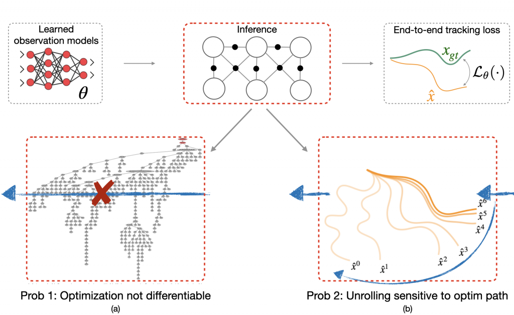
However, there are two problems with this approach. The first problem is that many state-of-the-art optimizers are not natively differentiable. For instance, the iSAM2 graph optimizer (Kaess 2012) used popularly for simultaneous localization and mapping (SLAM) invokes a series of non-differentiable Bayes tree operations and heuristics (Fig. 3a). Secondly, even if one did want to differentiate through the nonlinear optimizer, one would typically do this by unrolling successive optimization steps, and then propagating back gradients through the optimization procedure (Fig. 3b). However, training in this manner can have undesired effects. For example, prior work (Amos 2020) shows instances where even though unrolling gradient descent drives training loss to 0, the resulting cost landscape does not have a minimum on the ground truth. In other words, the learned cost landscape is sensitive to the optimization procedure used during training, e.g., the number of unrolling steps or learning rate.
Learning an energy landscape for the optimizer
We argue that instead of worrying about the optimization procedure, we should only care about the landscape of the energy or cost function that the optimizer has to minimize. We would like to learn an observation model that creates an energy landscape with a global minimum on the ground truth. This is precisely what energy-based models aim to do (LeCun 2006) and that is what we propose in our novel approach LEO that applies ideas from energy-based learning to our problem.
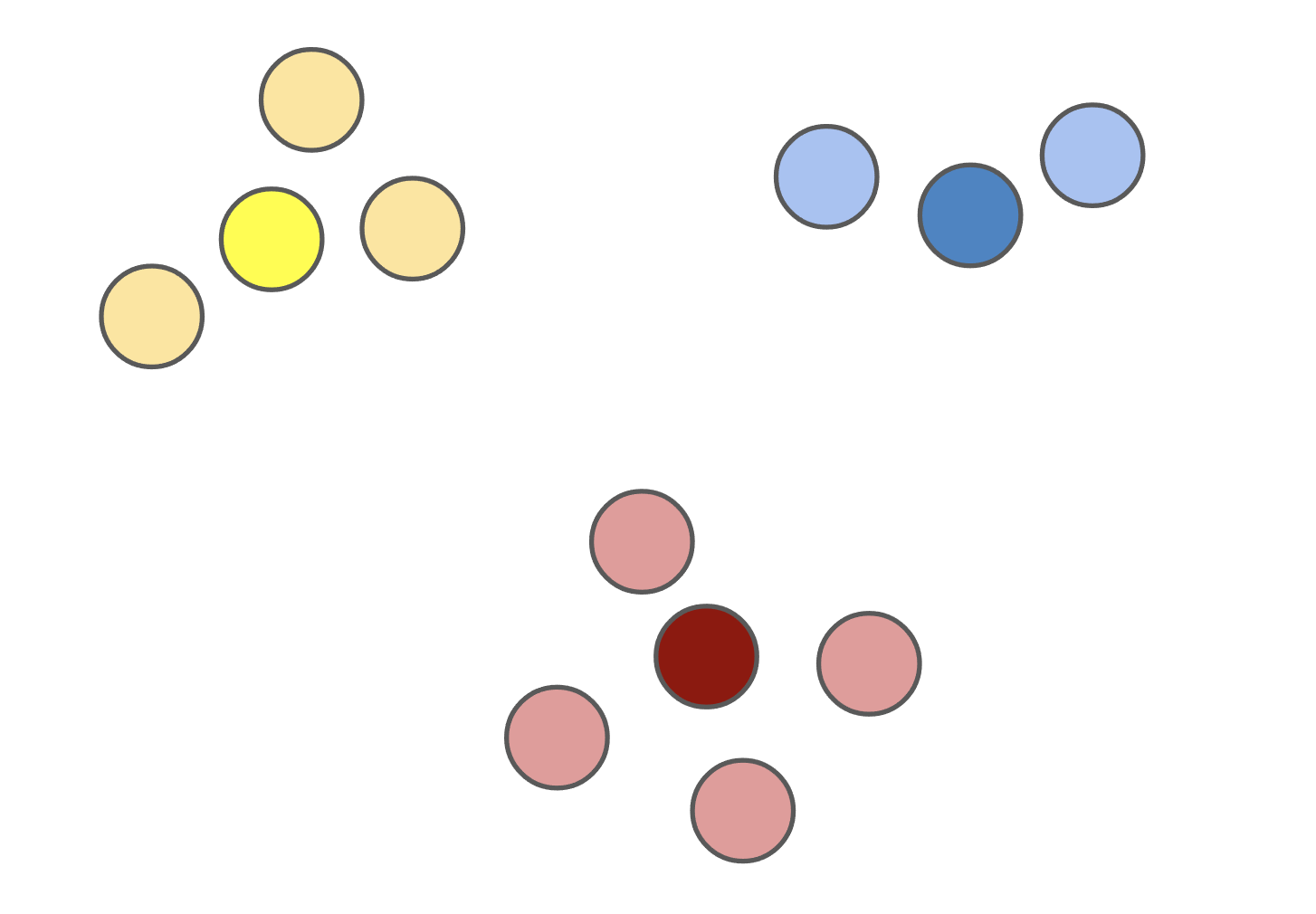
How does LEO work? Let us now demonstrate the inner workings of our approach on a toy example. For this, let us consider a one-dimensional visualization of the energy function represented in Fig 4. We collapse the trajectories down to a single axis. LEO begins by initializing with a random energy function. Note that the ground truth (x_{gt}) is far from the minimum. LEO samples trajectories (hat{x}) around the minimum by invoking the graph optimizer. It then compares these against ground truth trajectories and updates the energy function. The energy-based update rule is simple — push down the cost of ground truth trajectories (x_{gt}) and push up the cost of samples (hat{x}), with the cost of samples effectively acting as a contrastive term. If we keep iterating on this process, the minimum of the energy function eventually centers around the ground truth. At convergence, the gradients of the samples (hat{x}) on average match the gradient of the ground truth trajectory (x_{gt}). Since the samples are over a continuous space of trajectories for which exact computation of the log partition function is intractable, we propose a way to generate such samples efficiently using an incremental Gauss-Newton approximation (Kaess 2012).

How does LEO perform in practice? Let’s being with a simple regression problem (Amos 2020). We have pairs of ((x,y)) from a ground truth function (y=xsin(x)) and we would like to learn an energy function (E_theta(x,y)) such that (y = {operatorname{argmin}}_{y’} E_theta(x,y’)). LEO begins with a random energy function, but after a few iterations, learns an energy function with a distinct minimum around the ground truth function shown in solid line (Fig. 5). Contrast this to the energy functions learned by unrolling. Not only does it not have a distinct minimum around the ground truth, but it also varies with parameters like the number of unrolling iterations. This is because the learned energy landscape is specific to the optimization procedure used during learning.
Application to Robotics Problems
We evaluate LEO on two distinct robot applications, comparing it to baselines that either learn sequence-to-sequence networks or black-box search methods.
The first is a synthetic navigation task where the goal is to estimate robot poses from odometry and GPS observations. Here we are learning covariances, e.g., how noisy is GPS compared to odometry. Even though LEO is initialized far from the ground truth, it is able to learn parameters that pull the optimized trajectories close to the ground truth (Fig. 6).
We also look at a real-world manipulation task where an end-effector equipped with a touch sensor is pushing an object (Sodhi 2021). Here we learn a tactile model that maps a pair of tactile images to relative poses used in conjunction with physics and geometric priors. We show that LEO is able to learn parameters that pull optimized trajectories close to the ground truth or various object shapes and pushing trajectories (Fig. 7).
Parting Thoughts
While we focused on learning observation models for perception, the insights on learning energy landscapes for an optimizer extend to other domains such as control and planning. An increasingly unified view of robot perception and control is that both are fundamentally optimization problems. For perception, the objective is to optimize a sequence of states that explain the observations. For control, the objective is to optimize a sequence of actions that accomplish a task.
But what should the objective function be for both of these optimizations? Instead of hand designing observation models for perception or hand designing cost functions for control, we should leverage machine learning to learn these functions from data. To do so easily at scale, it is imperative that we build robotics pipelines and datasets that facilitate learning with optimizers in the loop.
Paper: https://arxiv.org/abs/2108.02274
Code+Video: https://psodhi.github.io/leo
References
[1] Dellaert and Kaess. Factor graphs for robot perception. Foundations and Trends in Robotics, 2017.[2] Kaess et al. iSAM2: Incremental smoothing and mapping using the Bayes tree. Intl. J. of Robotics Research (IJRR), 2012.
[3] LeCun et al. A tutorial on energy-based learning. Predicting structured data, 2006.
[4] Ziebart et al. Maximum entropy inverse reinforcement learning. AAAI Conf. on Artificial Intelligence, 2008.
[5] Amos and Yarats. The differentiable cross-entropy method. International Conference on Machine Learning (ICML), 2020.
[6] Yi et al. Differentiable factor graph optimization for learning smoothers. IEEE/RSJ Intl. Conf. on Intelligent Robots and Systems (IROS), 2021.
[7] Sodhi et al. Learning tactile models for factor graph-based estimation. IEEE Intl. Conf. on Robotics and Automation (ICRA), 2021.
[8] Lambeta et al. DIGIT: A novel design for a low-cost compact high-resolution tactile sensor with application to in-hand manipulation. IEEE Robotics and Automation Letters (RAL), 2020.
Perfecting pitch perception
New research from MIT neuroscientists suggests that natural soundscapes have shaped our sense of hearing, optimizing it for the kinds of sounds we most often encounter.
In a study reported Dec. 14 in the journal Nature Communications, researchers led by McGovern Institute for Brain Research associate investigator Josh McDermott used computational modeling to explore factors that influence how humans hear pitch. Their model’s pitch perception closely resembled that of humans — but only when it was trained using music, voices, or other naturalistic sounds.
Humans’ ability to recognize pitch — essentially, the rate at which a sound repeats — gives melody to music and nuance to spoken language. Although this is arguably the best-studied aspect of human hearing, researchers are still debating which factors determine the properties of pitch perception, and why it is more acute for some types of sounds than others. McDermott, who is also an associate professor in MIT’s Department of Brain and Cognitive Sciences, and an Investigator with the Center for Brains, Minds, and Machines (CBMM) at MIT, is particularly interested in understanding how our nervous system perceives pitch because cochlear implants, which send electrical signals about sound to the brain in people with profound deafness, don’t replicate this aspect of human hearing very well.
“Cochlear implants can do a pretty good job of helping people understand speech, especially if they’re in a quiet environment. But they really don’t reproduce the percept of pitch very well,” says Mark Saddler, a graduate student and CBMM researcher who co-led the project and an inaugural graduate fellow of the K. Lisa Yang Integrative Computational Neuroscience Center. “One of the reasons it’s important to understand the detailed basis of pitch perception in people with normal hearing is to try to get better insights into how we would reproduce that artificially in a prosthesis.”
Artificial hearing
Pitch perception begins in the cochlea, the snail-shaped structure in the inner ear where vibrations from sounds are transformed into electrical signals and relayed to the brain via the auditory nerve. The cochlea’s structure and function help determine how and what we hear. And although it hasn’t been possible to test this idea experimentally, McDermott’s team suspected our “auditory diet” might shape our hearing as well.
To explore how both our ears and our environment influence pitch perception, McDermott, Saddler, and Research Assistant Ray Gonzalez built a computer model called a deep neural network. Neural networks are a type of machine learning model widely used in automatic speech recognition and other artificial intelligence applications. Although the structure of an artificial neural network coarsely resembles the connectivity of neurons in the brain, the models used in engineering applications don’t actually hear the same way humans do — so the team developed a new model to reproduce human pitch perception. Their approach combined an artificial neural network with an existing model of the mammalian ear, uniting the power of machine learning with insights from biology. “These new machine-learning models are really the first that can be trained to do complex auditory tasks and actually do them well, at human levels of performance,” Saddler explains.
The researchers trained the neural network to estimate pitch by asking it to identify the repetition rate of sounds in a training set. This gave them the flexibility to change the parameters under which pitch perception developed. They could manipulate the types of sound they presented to the model, as well as the properties of the ear that processed those sounds before passing them on to the neural network.
When the model was trained using sounds that are important to humans, like speech and music, it learned to estimate pitch much as humans do. “We very nicely replicated many characteristics of human perception … suggesting that it’s using similar cues from the sounds and the cochlear representation to do the task,” Saddler says.
But when the model was trained using more artificial sounds or in the absence of any background noise, its behavior was very different. For example, Saddler says, “If you optimize for this idealized world where there’s never any competing sources of noise, you can learn a pitch strategy that seems to be very different from that of humans, which suggests that perhaps the human pitch system was really optimized to deal with cases where sometimes noise is obscuring parts of the sound.”
The team also found the timing of nerve signals initiated in the cochlea to be critical to pitch perception. In a healthy cochlea, McDermott explains, nerve cells fire precisely in time with the sound vibrations that reach the inner ear. When the researchers skewed this relationship in their model, so that the timing of nerve signals was less tightly correlated to vibrations produced by incoming sounds, pitch perception deviated from normal human hearing.
McDermott says it will be important to take this into account as researchers work to develop better cochlear implants. “It does very much suggest that for cochlear implants to produce normal pitch perception, there needs to be a way to reproduce the fine-grained timing information in the auditory nerve,” he says. “Right now, they don’t do that, and there are technical challenges to making that happen — but the modeling results really pretty clearly suggest that’s what you’ve got to do.”
This archaeologist fights tomb raiders with Google Earth
In the summer, Dr. Gino Caspari’s day starts at 5:30 a.m. in Siberia, where he studies the ancient Scythians with the Swiss National Science Foundation. There, he looks for burial places of these nomadic warriors who rode through Asia 2,500 years ago. The work isn’t easy, from dealing with extreme temperatures, to swamps covered with mosquitos. But the biggest challenge is staying one step ahead of tomb raiders.
It’s believed that more than 90% of the tombs — called kurgans — have already been destroyed by raiders looking to profit off what they find, but Gino is looking for the thousands he believes remain scattered across Russia, Mongolia and Western China. To track his progress, he began mapping these burial sites using Google Earth. “There’s a plethora of open data sources out there, but most of them don’t have the resolution necessary to detect individual archaeological structures,” Dr. Caspari says, pointing out that getting quality data is also very expensive. “Google Earth updates high-res data across the globe, and, especially in remote regions, it was a windfall for archaeologists. Google Earth expanded our possibilities to plan surveys and understand cultural heritage on a broader geographic scale.”
While Google Earth helped Dr. Caspari plan his expeditions, he still couldn’t stay ahead of the looters. He needed to get there faster. That’s when he met data scientist Pablo Crespo and started using another Google tool, TensorFlow.
“Since I started my PhD in 2013, I have been interested in automatic detection of archaeological sites from remote sensing data,” Gino says. “It was clear we needed to look at landscapes and human environmental interaction to understand past cultures. The problem was that our view was obscured by a lack of data and a focus on individual sites.” Back then, he tried some simple automatization processes to detect the places he needed for his research with the available technology, but only got limited results. In 2020, though, Gino and Pablo created a machine learning model using TensorFlow that could analyze satellite images they pulled from Google Earth. This model would look for places on the images that had the characteristics of a Scythian tomb.
The progress in the field of machine learning has been insanely fast, improving the quality of classification and detection to a point where it has become much more than just a theoretical possibility. Google’s freely available technologies have help
This technology sped up the discovery process for Gino, giving him an advantage over looters and even deterioration caused by climate change.
“Frankly, I think that without these tools, I probably wouldn’t have gotten this far in my understanding of technology and what it can do to make a difference in the study of our shared human past,” Gino says. “As a young scholar, I just lack the funds to access a lot of the resources I need. Working with Pablo and others has widened my perspective on what is possible and where we can go.”
Technology solutions have given Dr. Caspari’s work a new set of capabilities, supercharging what he’s able to do. And it’s also made him appreciate the importance of the human touch. “The deeper we dive into our past with the help of technology, the more apparent it becomes how patchy and incomplete our knowledge really is,” he says. “Technology often serves as an extension of our senses and mitigates our reality. Weaving the fabric of our reality will remain the task of the storyteller in us.”
ASRU: Integrating speech recognition and language understanding
Amazon’s Jimmy Kunzmann on how “signal-to-interpretation” models improve availability, performance.Read More
Top 5 Edge AI Trends to Watch in 2022
2021 saw massive growth in the demand for edge computing — driven by the pandemic, the need for more efficient business processes, as well as key advances in the Internet of Things, 5G and AI.
In a study published by IBM in May, for example, 94 percent of surveyed executives said their organizations will implement edge computing in the next five years.
From smart hospitals and cities to cashierless shops to self-driving cars, edge AI — the combination of edge computing and AI — is needed more than ever.
Businesses have been slammed by logistical problems, worker shortages, inflation and uncertainty caused by the ongoing pandemic. Edge AI solutions can be used as a bridge between humans and machines, enabling improved forecasting, worker allocation, product design and logistics.
Here are the top five edge AI trends NVIDIA expects to see in 2022:
1. Edge Management Becomes an IT Focus
While edge computing is rapidly becoming a must-have for many businesses, deployments remain in the early stages.
To move to production, edge AI management will become the responsibility of IT departments. In a recent report, Gartner wrote, “Edge solutions have historically been managed by the line of business, but the responsibility is shifting to IT, and organizations are utilizing IT resources to optimize cost.”1
To address the edge computing challenges related to manageability, security and scale, IT departments will turn to cloud-native technology. Kubernetes, a platform for containerized microservices, has emerged as the leading tool for managing edge AI applications on a massive scale.
Customers with IT departments that already use Kubernetes in the cloud can transfer their experience to build their own cloud-native management solutions for the edge. More will look to purchase third-party offerings such as Red Hat OpenShift, VMware Tanzu, Wind River Cloud Platform and NVIDIA Fleet Command.
2. Expansion of AI Use Cases at the Edge
Computer vision has dominated AI deployments at the edge. Image recognition led the way in AI training, resulting in a robust ecosystem of computer vision applications.
NVIDIA Metropolis, an application framework and set of developer tools that helps create computer vision AI applications, has grown its partner network 100-fold since 2017 to now include 1,000+ members.
Many companies are deploying or purchasing computer vision applications. Such companies at the forefront of computer vision will start to look to multimodal solutions.
Multimodal AI brings in different data sources to create more intelligent applications that can respond to what they see, hear and otherwise sense. These complex AI use cases employ skills like natural language understanding, conversational AI, pose estimation, inspection and visualization.
Combined with data storage, processing technologies, and input/output or sensor capabilities, multimodal AI can yield real-time performance at the edge for an expansion of use cases in robotics, healthcare, hyper-personalized advertising, cashierless shopping, concierge experiences and more.
Imagine shopping with a virtual assistant. With traditional AI, an avatar might see what you pick up off a shelf, and a speech assistant might hear what you order.
By combining both data sources, a multimodal AI-based avatar can hear your order, provide a response, see your reaction, and provide further responses based on it. This complementary information allows the AI to deliver a better, more interactive customer experience.
To see an example of this in action, check out Project Tokkio:
3. Convergence of AI and Industrial IoT Solutions
The intelligent factory is another space being driven by new edge AI applications. According to the same Gartner report, “By 2027, machine learning in the form of deep learning will be included in over 65 percent of edge use cases, up from less than 10 percent in 2021.”
Factories can add AI applications onto cameras and other sensors for inspection and predictive maintenance. However, detection is just step one. Once an issue is detected, action must be taken.
AI applications are able to detect an anomaly or defect and then alert a human to intervene. But for safety applications and other use cases when instant action is required, real-time responses are made possible by connecting the AI inference application with the IoT platforms that manage the assembly lines, robotic arms or pick-and-place machines.
Integration between such applications relies on custom development work. Hence, expect more partnerships between AI and traditional IoT management platforms that simplify the adoption of edge AI in industrial environments.
4. Growth in Enterprise Adoption of AI-on-5G
AI-on-5G combined computing infrastructure provides a high-performance and secure connectivity fabric to integrate sensors, computing platforms and AI applications — whether in the field, on premises or in the cloud.
Key benefits include ultra-low latency in non-wired environments, guaranteed quality-of-service and improved security.
AI-on-5G will unlock new edge AI use cases:
- Industry 4.0: Plant automation, factory robots, monitoring and inspection.
- Automotive systems: Toll road and vehicle telemetry applications.
- Smart spaces: Retail, smart city and supply chain applications.
One of the world’s first full stack AI-on-5G platforms, Mavenir Edge AI, was introduced in November. Next year, expect to see additional full-stack solutions that provide the performance, management and scale of enterprise 5G environments.
5. AI Lifecycle Management From Cloud to Edge
For organizations deploying edge AI, MLOps will become key to helping drive the flow of data to and from the edge. Ingesting new, interesting data or insights from the edge, retraining models, testing applications and then redeploying those to the edge improves model accuracy and results.
With traditional software, updates may happen on a quarterly or annual basis, but AI gains significantly from a continuous cycle of updates.
MLOps is still in early development, with many large players and startups building solutions for the constant need for AI technology updates. While mostly focused on solving the problem of the data center for now, such solutions in the future will shift to edge computing.
Riding the Next Wave of AI Computing
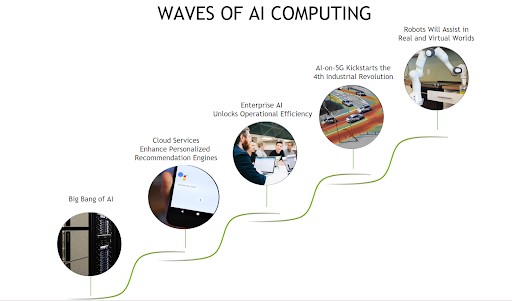
The development of AI has consisted of several waves, as pictured above.
Democratization of AI is underway, with new tools and solutions making it a reality. Edge AI, powered by huge growth in IoT and availability of 5G, is the next wave to break.
In 2022, more enterprises will move their AI inference to the edge, bolstering ecosystem growth as the industry looks at how to extend from cloud to the edge.
Learn more about edge AI by watching the GTC session, The Rise of Intelligent Edge: From Enterprise to Device Edge, on demand.
Check out NVIDIA edge computing solutions.
1 Gartner, “Predicts 2022: The Distributed Enterprise Drives Computing to the Edge”, 20 October 2021. By analysts: Thomas Bittman, Bob Gill, Tim Zimmerman, Ted Friedman, Neil MacDonald, Karen Brown
The post Top 5 Edge AI Trends to Watch in 2022 appeared first on The Official NVIDIA Blog.
BanditPAM: Almost Linear-Time k-medoids Clustering via Multi-Armed Bandits
TL;DR
Want something better than (k)-means? Our state-of-the-art (k)-medoids algorithm from NeurIPS, BanditPAM, is now publicly available! (texttt{pip install banditpam}) and you’re good to go!
Like the (k)-means problem, the (k)-medoids problem is a clustering problem in which our objective is to partition a dataset into disjoint subsets. In (k)-medoids, however, we require that the cluster centers must be actual datapoints, which permits greater interpretability of the cluster centers. (k)-medoids also works better with arbitrary distance metrics, so your clustering can be more robust to outliers if you’re using metrics like (L_1).
Despite these advantages, most people don’t use (k)-medoids because prior algorithms were too slow. In our NeurIPS paper, BanditPAM, we sped up the best known algorithm from (O(n^2)) to (O(ntext{log}n)).
We’ve released our implementation, which is pip-installable. It’s written in C++ for speed and supports parallelization and intelligent caching, at no extra complexity to end users. Its interface also matches the (texttt{sklearn.cluster.KMeans}) interface, so minimal changes are necessary to existing code.
Useful Links:
(k)-means vs. (k)-medoids
If you’re an ML practitioner, you’re probably familiar with the (k)-means problem. In fact, you may know some of the common algorithms for the (k)-means problem. You’re much less likely, however, familiar with the (k)-medoids problem.
The (k)-medoids problem is a clustering problem similar to (k)-means. Given a dataset, we want to partition our dataset into subsets where the points in each cluster are closer to a single cluster center than all other (k-1) cluster centers. Unlike in (k)-means, however, the (k)-medoids problem requires cluster centers to be actual datapoints.
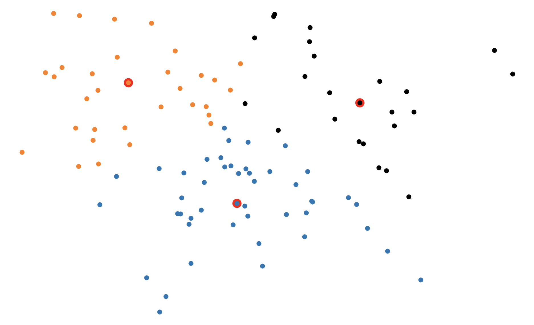
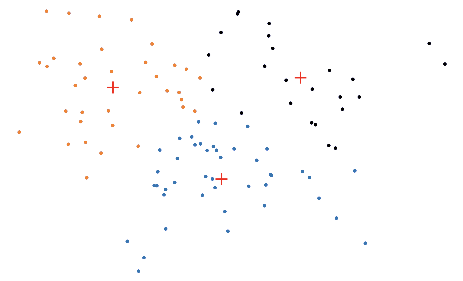
Figure 1: The (k)-medoids solution (left) forces the cluster centers to be actual datapoints. This solution is often different from the (k)-means solution (right).
The (k)-medoids problem has several advantages over (k)-means. By forcing the cluster centers — dubbed the medoids — to be actual datapoints, solutions tend to be more interpretable since you can determine exactly which datapoint is the cluster center for each cluster. When clustering images from the ImageNet dataset, for example, the mean of a solution to the (k)-means problem with (k = 1) are usually nondescript blobs (Figure 2, left), whereas the medoids of a corresponding solution to the (k)-medoids problem are actual images (Figure 2, right).


Figure 2: The cluster centers in (k)-means are often not easily interpretable, whereas they are actual datapoints in (k)-medoids. Shown are cluster centers for a subset of ImageNet with (k = 1) with (k)-means (top) and (k)-medoids (bottom). The mean of the dataset is the average per-pixel color, whereas the medoid is an image of a bee.
The (k)-medoids problem also supports arbitrary distance metrics, in contrast with (k)-means which usually requires (L_2) distance for efficiency. In fact, you’re allowed to use any pairwise dissimilarity function with (k)-medoids — your dissimilarity function need not even satisfy the properties of a metric. It can be asymmetric, negative, and violate the triangle inequality. In practice, allowing for arbitrary dissimilarity metrics enables the clustering of “exotic” objects like strings, natural language, trees, graphs, and more — without needing to embed these objects in a vector space first.
The advantages of (k)-medoids don’t stop there. Because the (k)-medoids problem supports arbitrary distance functions, the clustering can often be more robust to outliers if you’re using robust distance metrics. The (L_1) distance metric, for example, is more robust to outliers than the (L_2) distance metric; in one dimension, the (L_1) minimizer is the median of your datapoints whereas the (L_2) minimizer is the mean.
Despite all of these advantages, (k)-means is much more widely used than (k)-medoids, largely due to its much more favorable runtime. The best (k)-means algorithms scale linearly in dataset size, i.e., have (O(n)) complexity, whereas, until now, the best (k)-medoids algorithms scaled quadratically in dataset size, i.e., had (O(n^2)) complexity.
In our NeurIPS paper, BanditPAM, we reduced the complexity of the best known (k)-medoids algorithm from (O(n^2)) to (O(ntext{log}n)). This complexity almost matches the complexity of standard (k)-means algorithms — and now, you get all the benefits of (k)-medoids on top. We’ve also released a high-performance implementation of our algorithm written in C++ for speed but callable from Python via python bindings; (texttt{pip install banditpam}) and you’re ready to go! Our algorithm’s interface matches that of (texttt{sklearn.cluster.KMeans}) and can be used with a simple 2-line change. You can also implement your own distance metrics, interpret cluster centers, and cluster structured data!
BanditPAM: Almost Linear Time (k)-medoids Clustering via Multi-Armed Bandits
How does our algorithm, BanditPAM, work? Our claim is that we match the prior state-of-the-art solutions in clustering quality by recovering the exact same solution and reduce the complexity from (O(n^2)) to (O(ntext{log}n)). But is this reduction in complexity just “for free”?
To discuss how BanditPAM works, we first need to discuss its predecessor, the Partitioning Around Medoids (PAM) algorithm. The PAM algorithm, first proposed in 19901, is a greedy solution to the (k)-medoids problem. PAM is broken into two steps: the BUILD step and the SWAP step.
In the BUILD step, each of the (k) medoids is greedily initialized one by one. More concrete, PAM considers all possible datapoints as “candidate” medoids. For every candidate medoid, we compute the change in the overall loss if we were to add that candidate to the set of medoids conditioned on the previously assigned medoids being fixed. This results in an (O(n^2)) computational complexity since we need to compute every pairwise distance.
[In the SWAP step, we consider all (kn) (medoid, non-medoid) pairs and the change in loss that would be induced if we were to swap the first element of the pair out of the medoid set in favor of the second. Again, this procedure incurs an (O(n^2)) time complexity (really (O(kn^2))).
Figure 3: The (k)-medoids algorithm in action. In the BUILD step, each medoid is assigned greedily, one-by-one. In the SWAP step, we consider swapping medoid assignments to see if we can lower the overall loss.
Our fundamental insight was that for each step of the PAM algorithm, we don’t actually need to compute the distance from each point to all other (n) points. Instead, we can just sample these distances!
Consider, for example, the problem of assigning the first medoid at the beginning of the BUILD step. PAM would go through all (n) points and, for each point, compute its distance to every other point. We realized that, for each candidate, we only needed to compute the distance to (O(text{log}n)) other points. By intelligently choosing which distances to compute, we can save a lot of unnecessary computation. Formally, we reduce the problem of assigning the first medoid to a multi-armed bandit problem, as demonstrated in Figure 4. In multi-armed bandit problems, our objective is to identify the best action to take — also referred to as the best arm to pull — when actions are independent and have stochastic returns.
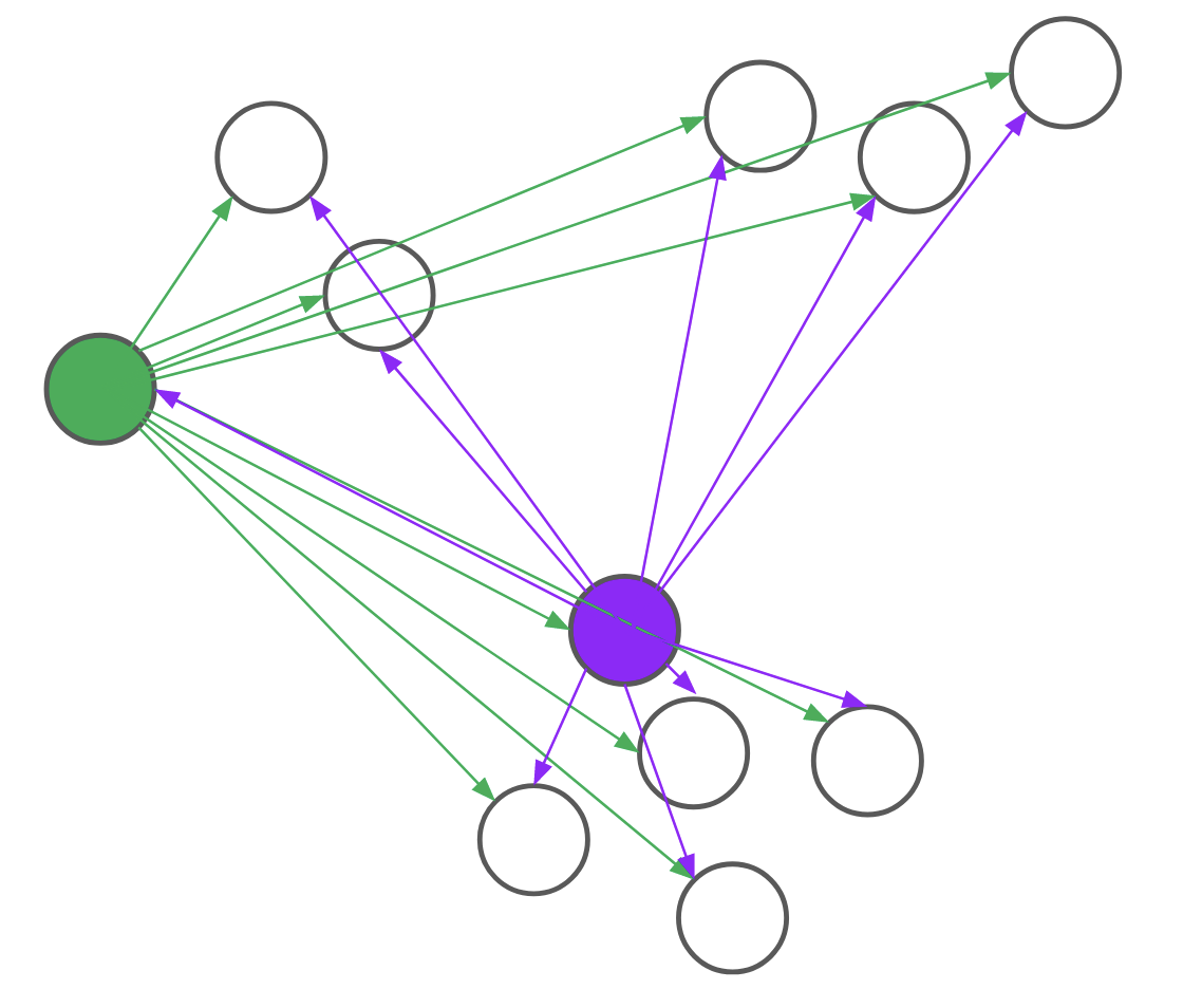
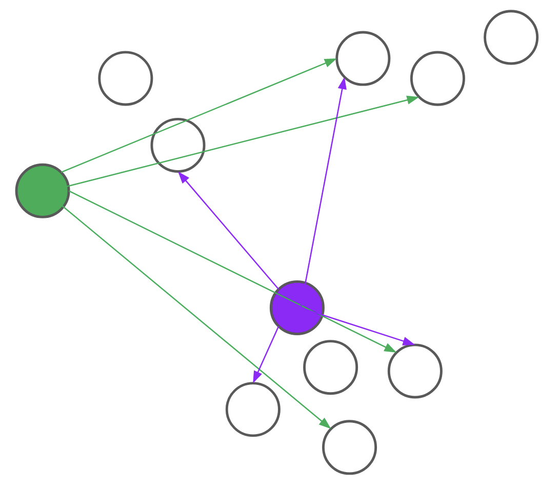
Figure 4: PAM (top) computes every pairwise distance for each candidate medoid. BanditPAM (bottom) only samples the pairwise distances. With just a few samples, we see that the purple point is a better candidate than the green point since the purple arrows are, on average, shorter than the green ones.
It turns out that all steps of the PAM algorithm can also be reduced to multi-armed bandit problems. In each part of the BUILD step, we still view each candidate datapoint as an arm. Now, however, pulling an arm corresponds to computing the induced change in loss for a random datapoint if we were to add the candidate to the set of medoids, conditioned on the previous medoids already being assigned. In each SWAP step, we view each (medoid, non-medoid) pair as an arm and pulling an arm corresponds to computing the induced change in loss on a random datapoint if we were to perform the swap. With these modifications, the original PAM algorithm is now reformulated as a sequence of best-arm identification problems. This reformulation reduces every step of the PAM algorithm from (O(n^2)) to (O(nlogn)).
Now, if you’re familiar with multi-armed bandits, you might protest. Our algorithm is a randomized algorithm and can sometimes return an incorrect result. In the full paper, we show that the probability of getting a “wrong” answer is very small. In practice, this means that users of our algorithm don’t have to worry and will almost always get the same answer as the original PAM algorithm.
The BanditPAM algorithm is an (O(ntext{log}n)) algorithm that matches prior state-of-the-art algorithms in clustering quality and almost matches the complexity of popular (k)-means algorithms. Want to try out BanditPAM? Run (texttt{pip3 install banditpam}) and jump to our examples.

Figure 5: A formal proof that (k)-medoids is superior to (k)-means in every way.
Acknowledgments
This blog post is based on the paper: BanditPAM: Almost Linear Time (k)-medoids Clustering via Multi-Armed Bandits. NeurIPS 2021.
A special thanks to my collaborators on this project, Martin Jinye Zhang, James Mayclin, Sebastian Thrun, Chris Piech, and Ilan Shomorony, as well as the reviewers of this blog post, Drew A. Hudson and Sidd Karamcheti.
-
Kaufman, Leonard; Rousseeuw, Peter J. (1990-03-08), “Partitioning Around Medoids (Program PAM)”, Wiley Series in Probability and Statistics, Hoboken, NJ, USA: John Wiley & Sons, Inc., pp. 68–125] ↩