Every living cell contains its own bustling microcosm, with thousands of components responsible for energy production, protein building, gene transcription and more.
Scientists at the University of Illinois at Urbana-Champaign have built a 3D simulation that replicates these physical and chemical characteristics at a particle scale — creating a fully dynamic model that mimics the behavior of a living cell.
Published in the journal Cell, the project simulates a living minimal cell, which contains a pared-down set of genes essential for the cell’s survival, function and replication. The model uses NVIDIA GPUs to simulate 7,000 genetic information processes over a 20-minute span of the cell cycle – making it what the scientists believe is the longest, most complex cell simulation to date.
Minimal cells are simpler than naturally occurring ones, making them easier to recreate digitally.
“Even a minimal cell requires 2 billion atoms,” said Zaida Luthey-Schulten, chemistry professor and co-director of the university’s Center for the Physics of Living Cells. “You cannot do a 3D model like this in a realistic human time scale without GPUs.”
Once further tested and refined, whole-cell models can help scientists predict how changes to the conditions or genomes of real-world cells will affect their function. But even at this stage, minimal cell simulation can give scientists insight into the physical and chemical processes that form the foundation of living cells.
“What we found is that fundamental behaviors emerge from the simulated cell — not because we programmed them in, but because we had the kinetic parameters and lipid mechanisms correct in our model,” she said.
Lattice Microbes, the GPU-accelerated software co-developed by Luthey-Schulten and used to simulate the 3D minimal cell, is available on the NVIDIA NGC software hub.
Minimal Cell With Maximum Realism
To build the living cell model, the Illinois researchers simulated one of the simplest living cells, a parasitic bacteria called mycoplasma. They based the model on a trimmed-down version of a mycoplasma cell synthesized by scientists at J. Craig Venter Institute in La Jolla, Calif., which had just under 500 genes to keep it viable.
For comparison, a single E. coli cell has around 5,000 genes. A human cell has more than 20,000.
Luthy-Schulten’s team then used known properties of the mycoplasma’s inner workings, including amino acids, nucleotides, lipids and small molecule metabolites to build out the model with DNA, RNA, proteins and membranes.
“We had enough of the reactions that we could reproduce everything known,” she said.
Using Lattice Microbes software on NVIDIA Tensor Core GPUs, the researchers ran a 20-minute 3D simulation of the cell’s life cycle, before it starts to substantially expand or replicate its DNA. The model showed that the cell dedicated most of its energy to transporting molecules across the cell membrane, which fits its profile as a parasitic cell.
“If you did these calculations serially, or at an all-atom level, it’d take years,” said graduate student and paper lead author Zane Thornburg. “But because they’re all independent processes, we could bring parallelization into the code and make use of GPUs.”
Thornburg is working on another GPU-accelerated project to simulate growth and cell division in 3D. The team has recently adopted NVIDIA DGX systems and RTX A5000 GPUs to further accelerate its work, and found that using A5000 GPUs sped up the benchmark simulation time by 40 percent compared to a development workstation with a previous-generation NVIDIA GPU.
Learn more about researchers using NVIDIA GPUs to accelerate science breakthroughs by registering free for NVIDIA GTC, running online March 21-24.
Main image is a snapshot from the 20-minute 3D spatial simulation, showing yellow and purple ribosomes, red and blue degradasomes, and smaller spheres representing DNA polymers and proteins.
This GFN Thursday brings the launch of Tom Clancy’s Rainbow Six Extraction to GeForce NOW.
Plus, four new games are joining the GeForce NOW library to let you start your weekend off right.
Your New Mission, Should You Choose to Accept It
Grab your gadgets and get ready to game. Tom Clancy’s Rainbow Six Extraction releases today and is available to stream on GeForce NOW with DLSS for higher frame rates and beautiful, sharp images.
Join millions of players in the Rainbow Six universe. Charge in on your own or battle with buddies in a squad of up to three in thrilling co-op gameplay.
Select from 18 different Operators with specialized skills and progression paths that sync with your strategy to take on different challenges. Play riveting PvE on detailed containment zones, collect critical information and fight an ever-evolving, highly lethal alien threat known as the Archaeans that’s reshaping the battlefield.
Playing With the Power of GeForce RTX 3080
Members can stream Tom Clancy’s Rainbow Six Extraction and the 1,100+ games on the GeForce NOW library, including nearly 100 free-to-play titles, with all of the perks that come with the new GeForce NOW RTX 3080 membership.
Build your team, pick your strategy and complete challenging missions in Tom Clancy’s Rainbow Six Extraction.
This new tier of service allows members to play across their devices – including underpowered PCs, Macs, Chromebooks, SHIELD TVs, Android devices, iPhones or iPads – with the power of GeForce RTX 3080. That means benefits like ultra-low latency and eight-hour gaming sessions — the longest available — for a maximized experience on the cloud.
Plus, RTX 3080 members have the ability to fully control and customize in-game graphics settings, with RTX ON rendering environments in cinematic quality for supported games.
We make every effort to launch games on GeForce NOW as close to their release as possible, but, in some instances, games may not be available immediately.
Finally, we’ve got a question for you and your gaming crew this week. Talk to us on Twitter or in the comments below.
~𝙬𝙝𝙤𝙡𝙚𝙨𝙤𝙢𝙚 𝙩𝙝𝙧𝙚𝙖𝙙~
tag a squadmate you’re grateful for and tell them why
Robotaxis are on their way to delivering safer transportation, driving across various landscapes and through starry nights.
This week, Silicon Valley-based self-driving startup Pony.ai announced its next-generation autonomous computing platform, built on NVIDIA DRIVE Orin for high-performance and scalable compute. The centralized system will serve as the brain for a robotaxi fleet of Toyota Sienna multipurpose vehicles (MPVs), marking a major leap forward for the nearly six-year-old company.
The AI compute platform enables multiple configurations for scalable autonomous driving development, all the way to level 4 self-driving vehicles.
“By leveraging the world-class NVIDIA DRIVE Orin SoC, we’re demonstrating our design and industrialization capabilities and ability to develop and deliver a powerful mass-production platform at an unprecedented scale,” said James Peng, co-founder and CEO of Pony.ai, which is developing autonomous systems for both robotaxis and trucks.
The transition to DRIVE Orin has significantly accelerated the company’s plans to deploy safer, more efficient robotaxis, with road testing set to begin this year in China and commercial rollout planned for 2023.
State-of-the-Art Intelligence
DRIVE Orin serves as the brain of autonomous fleets, enabling them to perceive their environment and continuously improve over time.
Born out of the data center, DRIVE Orin achieves 254 trillions of operations per second, or TOPS. It’s designed to handle the large number of applications and deep neural networks that run simultaneously in autonomous trucks, while achieving systematic safety standards such as ISO 26262 ASIL-D.
Pony.ai’s DRIVE Orin-based autonomous computing unit features low latency, high performance and high reliability. It also incorporates a robust sensor solution that contains more than 23 sensors, including solid-state lidars, near-range lidars, radars and cameras.
The Pony.ai next-generation autonomous computing platform, built on NVIDIA DRIVE Orin.
This next-generation, automotive-grade system incorporates redundancy and diversity, maximizing safety while increasing performance and reducing weight and cost over previous iterations.
A Van for All Seasons
The Toyota Sienna MPV is a prime candidate for robotaxi services as it offers flexibility and ride comfort in a sleek package.
Toyota and Pony.ai began co-developing Sienna vehicles purpose-built for robotaxi services in 2019. The custom vehicles feature a dual-redundancy system and better control performance for level 4 autonomous driving capabilities.
The vehicles also debut new concept design cues, including rooftop signaling units that employ different colors and lighting configurations to communicate the robotaxi’s status and intentions.
This dedicated, future-forward design combined with the high-performance compute of NVIDIA DRIVE Orin lays a strong foundation for the coming generation of safer, more efficient robotaxi fleets.
Capacity is a key component of reliability. Uber’s services require enough resources in order to handle daily peak traffic and to support our different kinds of business units. These services are deployed across different cloud platforms and data centers …
In the last three years, the largest trained dense models have increased in size by over 1,000 times, from a few hundred million parameters to over 500 billion parameters in Megatron-Turing NLG 530B (MT-NLG). Improvements in model quality with size suggest that this trend will continue, with larger model sizes bringing better model quality. However, sustaining the growth in model size is getting more difficult due to the increasing compute requirements.
There have been numerous efforts to reduce compute requirements to train large models without sacrificing model quality. To this end, architectures based on Mixture of Experts (MoE) have paved a promising path, enabling sub-linear compute requirements with respect to model parameters and allowing for improved model quality without increasing training cost.
However, MoE models have their own challenges. First, the scope of MoE models is primarily limited on encoder-decoder models and sequence-to-sequence tasks. Second, MoE models require more parameters to achieve the same model quality as their dense counterparts, which requires more memory for training and inference even though MoE models require less compute. Lastly, a critical consideration is that MoE models’ large size makes inference difficult and costly.
To address these above challenges, the DeepSpeed team, as part of Microsoft’s AI at Scale initiative, has been exploring new applications and optimizations for MoE models at scale. These can lower the training and inference cost of large models, while also enabling the ability to train and serve the next generation of models affordably on today’s hardware. Here, we are happy to share our findings and innovations for MoE models and systems that 1) reduce training cost by 5x, 2) reduce MoE parameter size by up to 3.7xand 3) reduce MoE inference latency by 7.3x at an unprecedented scale and offer up to 4.5x faster and 9x cheaper inference for MoE models compared to quality-equivalent dense models:
5x reduction in training cost for natural language generation (NLG) models: We extend the scope of MoE models to beyond just encoder-decoder models and sequence-to-sequence tasks, demonstrating that MoE can reduce the training cost of NLG models like those in the GPT family or MT-NLG by 5x while obtaining the same model quality. Data scientists can now train models of superior quality previously only possible with 5x more hardware resources.
Reduced model size and improved parameter efficiency with Pyramid-Residual-MoE (PR-MoE)Architecture and Mixture-of-Students (MoS):The training cost reduction of MoE is not free and comes at the expense of increasing the total number of parameters required to achieve the same model quality as dense models. PR-MoE is a hybrid dense and MoE model created using residual connections, applying experts only where they are most effective. PR-MoE reduces MoE model parameter size by up to 3x with no change to model quality. In addition, we leverage staged knowledge distillation to learn a Mixture-of-Students model that further leads to up to 3.7x model size reduction while retaining similar model quality.
Fast and economical MoE inference at unprecedented scale: The DeepSpeed-MoE (DS-MoE) inference system enables efficient scaling of inference workloads on hundreds of GPUs, providing up to 7.3x reduction in inference latency and cost when compared with existing systems. It offers ultra-fast inference latencies (25 ms) for trillion-parameter MoE models. DS-MoE also offers up to 4.5x faster and 9x cheaper inference for MoE models compared to quality-equivalent dense models by combining both system and model optimizations.
Each of these advances is explored further in the blog post below. For more about the technical details, please read our paper.
DeepSpeed-MoE for NLG: Reducing the training cost of language models by five times
While recent works like GShard and Switch Transformers have shown that the MoE model structure can reduce large model pretraining cost for encoder-decoder model architecture, their impact on the much more compute-intensive transformer-based autoregressive NLG models has been mostly unknown.
Given the tremendous compute and energy requirements for training NLG models, we explore opportunities where MoE can reduce their training cost. We show that MoE can be applied to NLG models to significantly improve their model quality with the same training cost. Also, MoE can achieve 5x reduction in training cost to achieve the same model quality of a dense NLG model. For example, we achieved the quality of a 6.7B-parameter dense NLG model at the cost of training a 1.3B-parameter dense model. Our observation about MoE training cost savings aligns with parallel explorations from Du et al. and Artetxe et al., where they also demonstrated the savings for models with bigger sizes.
Our MoE-based NLG model architecture
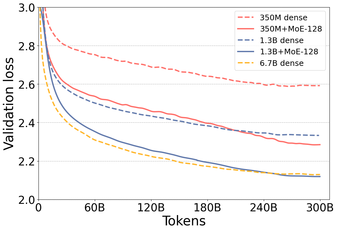
To create an MoE-based NLG model, we studied a transformer-based NLG model similar to those of the GPT family. To complete training in a reasonable timeframe, the following models were selected: 350M (24 layers, 1024 hidden size, 16 attention heads), 1.3B (24 layers, 2048 hidden size, 16 attention heads), and 6.7B (32 layers, 4096 hidden size, 32 attention heads). We use “350M+MoE-128” to denote a MoE model that uses 350M dense model as the base model and adds 128 experts on every other feedforward layer.
MoE training infrastructure and dataset
We pretrained both the dense and MoE versions of the above models using DeepSpeed on 128 NVIDIA Ampere A100 GPUs (Azure ND A100 instances). These Azure instances are powered by the latest Azure HPC docker images that provide a fully optimized environment and best performing library versions of NCCL, Mellanox OFED, Sharp, and CUDA. DeepSpeed uses a combination of data-parallel and expert-parallel training to effectively scale MoE model training and is capable of training MoE models with trillions of parameters on hundreds of GPUs.
We used the same training data as described in the MT-NLG blog post. For a fair comparison, we use 300 billion tokens to train both dense and MoE models.
MoE leads to better quality for NLG models
Figure 1 shows that the validation loss for the MoE versions of the model is significantly better than their dense counterparts. Furthermore, validation loss of the 350M+MoE-128 model is on par validation loss of the 1.3B dense model with 4x larger base. This is also true for 1.3B+MoE-128 in comparison with 6.7B dense model with 5x larger base. Furthermore, the model quality is on par not only with the validation loss but also with six zero-shot evaluation tasks as shown in Table 1, demonstrating that these models have very similar model quality.
Case
Model size
LAMBADA: completion prediction
PIQA: commonsense reasoning
BoolQ: reading comprehension
RACE-h: reading comprehension
TriviaQA: question answering
WebQs: question answering
Dense NLG:
(1) 350M
350M
0.5203
0.6931
0.5364
0.3177
0.0321
0.0157
(2) 1.3B
1.3B
0.6365
0.7339
0.6339
0.3560
0.1005
0.0325
(3) 6.7B
6.7B
0.7194
0.7671
0.6703
0.3742
0.2347
0.0512
Standard MoE NLG:
(4) 350M+MoE-128
13B
0.6270
0.7459
0.6046
0.3560
0.1658
0.0517
(5) 1.3B+MoE-128
52B
0.6984
0.7671
0.6492
0.3809
0.3129
0.0719
PR-MoE NLG:
(6) 350M+PR-MoE-32/64
4B
0.6365
0.7399
0.5988
0.3569
0.1630
0.0473
(7) 1.3B+PR-MoE-64/128
31B
0.7060
0.7775
0.6716
0.3809
0.2886
0.0773
PR-MoE NLG + MoS:
(8) 350M+PR-MoE-32/64 + MoS-21L
3.5B
0.6346
0.7334
0.5807
0.3483
0.1369
0.0522
(9) 1.3B+PR-MoE-64/128 + MoS-21L
27B
0.7017
0.7769
0.6566
0.3694
0.2905
0.0822
Table 1: Zero-shot evaluation results (last six columns) for different dense and MoE NLG models. All zero-shot evaluation results use the accuracy metric.
Figure 1: Token-wise validation loss curves for dense and MoE NLG models with different model sizes.
Same quality with 5x less training cost
As shown in the results above, adding MoE with 128 experts to the NLG model significantly improves its quality. However, these experts do not change the compute requirements of the model as each token is only processed by a single expert. Therefore, the compute requirements for a dense model and its corresponding MoE models with the same base are similar.
More concretely, training 1.3B+MoE-128 requires roughly the same amount of compute operations as a 1.3B dense model while offering much better quality. Our results show that by applying MoE, the model quality of a 6.7B-parameter dense model can be achieved at the training cost of a 1.3B-parameter dense model, resulting in an effective training compute reduction of 5x.
This compute cost reduction can directly be translated into throughput gain, training time and training cost reduction by leveraging the efficient DeepSpeed MoE training system. Table 2 shows the training throughput of 1.3B+MoE-128 compared with the 6.7B dense model on 128 NVIDIA A100 GPUs.
Training samples per sec
Throughput gain/ Cost Reduction
6.7B dense
70
1x
1.3B+MoE-128
372
5x
Table 2: Training throughput (on 128 A100 GPUs) of an MoE-based model versus a dense model, where both achieve the same model quality.
PR-MoE and Mixture-of-Students: Reducing the model size and improving parameter efficiency
While MoE-based models achieve the same quality with 5x training cost reduction in the NLG example, the resulting model has roughly 8x the parameters of the corresponding dense model. For example, a 6.7B dense model has 6.7 billion parameters and 1.3B+MoE-128 has 52 billion parameters. Training such a massive MoE model requires significantly more memory; inference latency and cost could also increase since the primary inference bottleneck is often the memory bandwidth needed to read model weights.
To reduce model size and improve parameter efficiency, we’ve made innovations in the MoE model architecture that reduce the overall model size by up to 3 times without affecting model quality. We also leverage knowledge distillation to learn a Mixture-of-Students (MoS) model, with a smaller model capacity as the teacher PR-MoE but preserve the teacher model accuracy.
Two intuitions for improving MoE architecture
Intuition-I: The standard MoE architecture has the same number and structure of experts in all MoE layers. This relates to a fundamental question in the deep learning community, which has been well-studied in computer vision: do all the layers in a deep neural network learn the same representation? Shallow layers learn general representations and deep layers learn more objective-specific representations. This also leads transfer learning in computer vision to freeze shallow layers for fine-tuning. This phenomenon, however, has not been well-explored in natural language processing (NLP), particularly for MoE.
To investigate the question, we compare the performance of two different half-MoE architectures. More specifically, we put MoE layers in the first half of the model and leave the second half’s layers identical to the dense model. We switch the MoE layers to the second half and use dense at the first half. The results show that deeper layers benefit more from large number of experts. This confirms that not all MoE layers learn the same level of representations.
Intuition-II: To improve the generalization performance of MoE models, there are two common methods: 1) increasing the number of experts while keeping the capacity (that is, for each token, the number of experts it goes through) to be the same; 2) doubling the capacity at the expense of slightly more computation (33%) while keeping the same number of experts. However, for method 1, the memory requirement for training resources needs to be increased due to larger number of experts. For method 2, higher capacity also doubles the communication volume which can significantly slow down training and inference. Is there a way to keep the training and inference efficiency while getting generalization performance gain?
One intuition of why larger capacity helps accuracy is that those extra experts can help correct the “representation” of the first expert. However, does this first expert need to be changed every time? Or can we fix the first and only assign different extra experts to different tokens?
To investigate this, we perform a comparison in two ways: doubling the capacity and fixing one expert while varying the second expert across different experts. For the latter, a token will always pass a dense multilayer perceptron (MLP) module and an expert from MoE module. Therefore, we can achieve the benefit of using two experts per layer but still use one communication. We find out that the generalization performance of these two is on-par with each other. However, the training/inference speed of our new design is faster.
New MoE Architecture: Pyramid-Residual MoE
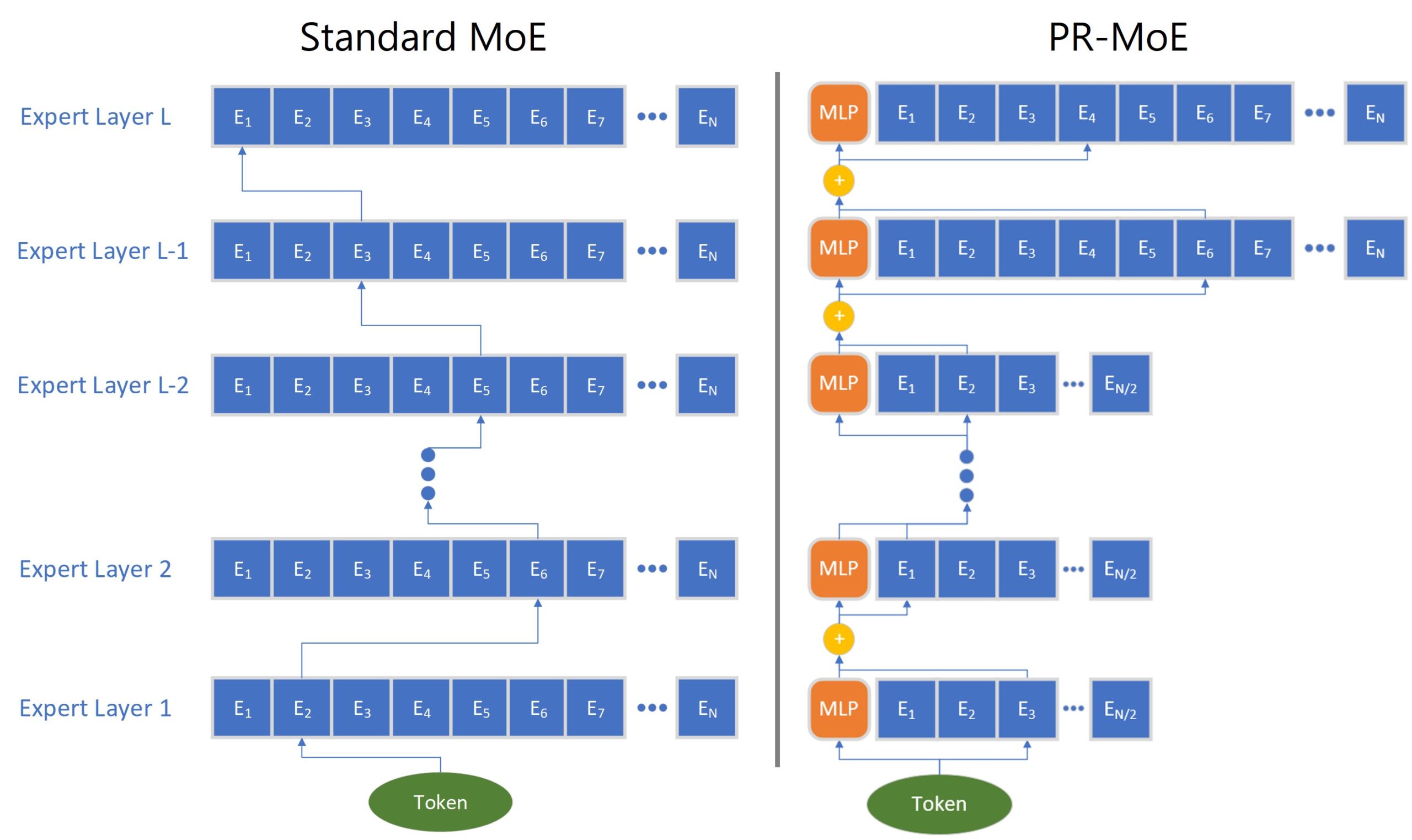
We propose a novel MoE architecture, Pyramid-Residual MoE (PR-MoE). Figure 2 (right) shows its architecture. Following Intuition-I, PR-MoE utilizes more experts in the last few layers as compared to previous layers, which gives a reverse pyramid design. Following Intuition II, we propose a Residual-MoE structure, where each token separately passes one fixed MLP layer and one chosen expert. Combining them results in the PR-MoE model, where all standard MoE layers are replaced by the new PR-MoE layer.
Figure 2: The illustration of standard MoE (left) and PR-MoE (right).
Same quality as standard models with up to 3x model size reduction: We evaluate PR-MoE on two model sizes, with bases of 350M and 1.3B parameters, and compare the performance with larger standard MoE architectures. The results are shown in Table 1 above. For both cases, PR-MoE uses much fewer experts but achieves comparable accuracy as standard MoE models. In the 350M model, PR-MoE only uses less than one third of the parameters that the standard MoE uses. In the 1.3B case, PR-MoE only uses about 60 percent of the parameters required for standard MoE.
Mixture-of-Students: Distillation for even smaller model size and faster inference
Model compression and distillation present additional opportunities to improve inference performance further. While there are many ways for model compression, such as quantization and pruning, we focus on reducing the number of layers of each expert in MoE and using knowledge distillation to compress the resulting student model to achieve a similar performance to the teacher MoE.
Since MoE structure brings significant benefits by enabling sparse training and inference, our task-agnostic distilled MoE model, which we call Mixture of Students (MoS), inherits these benefits while still providing the flexibility to compress into a dense model. We note that while existing work primarily considers small transformers (a few hundred parameters) and dense encoder-based LM models (like BERT), we focus on studying knowledge distillation for sparse MoE-based auto-generative language models on a multi-billion parameter scale. Furthermore, given the excellent performance of PR-MoE, we combine PR-MoE with MoS to further reduce the MoE model size.
To apply knowledge distillation for MoE, we first train a teacher MoE model using the same training hyperparameters and datasets as in the previous section. The teacher model is 350M+PR-MoE-32/64 and 1.3B+PR-MoE-64/128, respectively. We reduce the depth of the teacher model to 21 (12.5%) to obtain a student model, and we force the student to imitate the outputs from the teacher MoE on the training dataset.
In particular, we take the knowledge distillation loss as a weighted sum of the cross-entropy loss between predictions and the given hard label and the Kullback–Leibler (KL) divergence loss between the predictions and the teacher’s soft label. In practice, we observe that distillation may adversely affect MoS accuracy. In particular, while knowledge distillation loss improves validation accuracy initially, it begins to hurt accuracy towards the end of training.
We hypothesize that because the PR-MoE already reduces the capacity compared with the standard MoE by exploiting the architecture change (for example, reducing experts in lower layers), further reducing the depth of the model causes the student to have insufficient capacity, making it fall into the underfitting regime. Therefore, we take a staged distillation approach, where we decay the impact from knowledge distillation gradually in the training process.
Our study shows that it is possible to reach similar performance—such as in zero-shot evaluation on many downstream tasks—for a smaller MoE model pretrained with knowledge distillation. The MoS achieve comparable accuracy to the teacher MoE model, retaining 99.3% and 99.1% of the performance despite having 12.5% fewer layers. This enables an additional 12.5% model size reduction. When combined with PR-MoE, it leads to up to 3.7x model size reduction.
DeepSpeed-MoE inference: Serving MoE models at unprecedented scale and speed
Optimizing for MoE inference latency and cost is crucial for MoE models to be useful in practice. During inference the batch size is generally small, so the inference latency of an MoE model depends primarily on time it takes to load the model parameters from main memory, contrasting with the conventional belief that lesser compute should lead to faster inference. So, inference performance mainly depends on two factors: the overall model size and the overall achievable memory bandwidth.
In the previous section, we presented PR-MoE and distillation to optimize the model size. This section presents our solution to maximize the achievable memory bandwidth by creating a multi-GPU MoE inferencing system that can leverage the aggregated memory bandwidth across dozens of distributed GPUs to speed up inference. Together, DeepSpeed offers an unprecedented scale and efficiency to serve massive MoE models with 7.3x better latency and cost compared to baseline MoE systems, and up to 4.5x faster and 9x cheaper MoE inference compared to quality-equivalent dense models.
MoE inference performance is an interesting paradox
From the best-case view, each token of an MoE model only activates a single expert at each MoE layer, resulting in a critical data path that is equivalent to the base model size, orders-of-magnitude smaller than the actual model size. For example, when inferencing with a 1.3B+MoE-128 model, each input token needs just 1.3 billion parameters, even though the overall model size is 52 billion parameters.
From the worst-case view, the aggregate parameters needed to process a group of tokens can be as large as the full model size, in the example, the entire 52 billion parameters, making it challenging to achieve short latency and high throughput.
Design goals for the DS-MoE inference system
The design goal of our optimizations is to steer the performance toward the best-case view. This requires careful orchestration and partitioning of the model to group and route all tokens with the same critical data path together to reduce data access per device and achieve maximum aggregate bandwidth. An overview of how DS-MoE tackles this design goal by embracing multi-dimensional parallelism inherent in MoE models is illustrated in Figure 3.
Figure 3: DS-MoE design that embraces the complexity of multi-dimensional parallelism for different partitions (expert and non-expert) of the model.
DS-MoE inference system is centered around three well-coordinated optimizations:
The DS-MoE Inference system is designed to minimize the critical data path per device and maximize the achievable aggregate memory bandwidth across devices, which is achieved by: 1) expert parallelism and expert-slicing on expert parameters and 2) data parallelism and tensor-slicing for non-expert parameters.
Expert parallelism and expert-slicing for expert parameters: We partition experts across devices, group all tokens of using the same experts under the same critical data path, and parallelize processing of the token groups with different critical paths among different devices using expert parallelism.
In the example of 1.3B+MoE-128, when expert parallelism is equal to 128, each GPU only processes a single token group corresponding to the experts on that device. This results in a sequential path that is 1.3 billion parameters per device, 5x smaller than its quality-equivalent dense model with 6.7B parameters. Therefore, in theory, an MoE-based model has the potential to run up to 5x faster than its quality-equivalent dense model using expert parallelism assuming no communication overhead, a topic we discuss in the next section.
In addition, we propose “expert-slicing” to leverage the concept of tensor-slicing for the parameters within an expert. This additional dimension of parallelism is helpful for latency stringent scenarios that we scale to more devices than the number of experts.
Data parallelism and Tensor-slicing for non-expert parameters: Within a node, we use tensor-slicing to partition the non-expert parameters, leveraging aggregate GPU memory bandwidth of all GPUs to accelerate the processing. While it is possible to perform tensor-slicing across nodes, the communication overhead of tensor-slicing along with reduced compute granularity generally makes inter-node tensor-slicing inefficient. To scale non-expert parameters across multiple nodes, we use data parallelism by creating non-expert parameter replicas processing different batches across nodes that incurs no communication overhead or reduction in compute granularity.
Figure 3 above shows an example scenario for distributed MoE inference highlighting different parts of the MoE model, how the model and data are partitioned, and what form of parallelism is used to deal with each piece.
Microsoft Collective Communication Library (MSCCL) is a platform to execute custom collective communication algorithms for multiple accelerators supported by Microsoft Azure.
Expert parallelism requires all-to-all communication between all expert parallel devices. By default, DS-MoE uses NCCL for this communication via torch. distributed interface, but we observe major overhead when it is used at scale. To optimize this, we develop a custom communication interface to use Microsoft SCCL and achieve better performance than NCCL. Despite the plug-in optimizations, it is difficult to scale expert parallelism to many devices as the latency increases linearly with the increase in devices. To address this critical scaling challenge, we design two new communication optimization strategies that exploit the underlying point-to-point NCCL operations and custom CUDA kernels to perform necessary data-layout transformations.
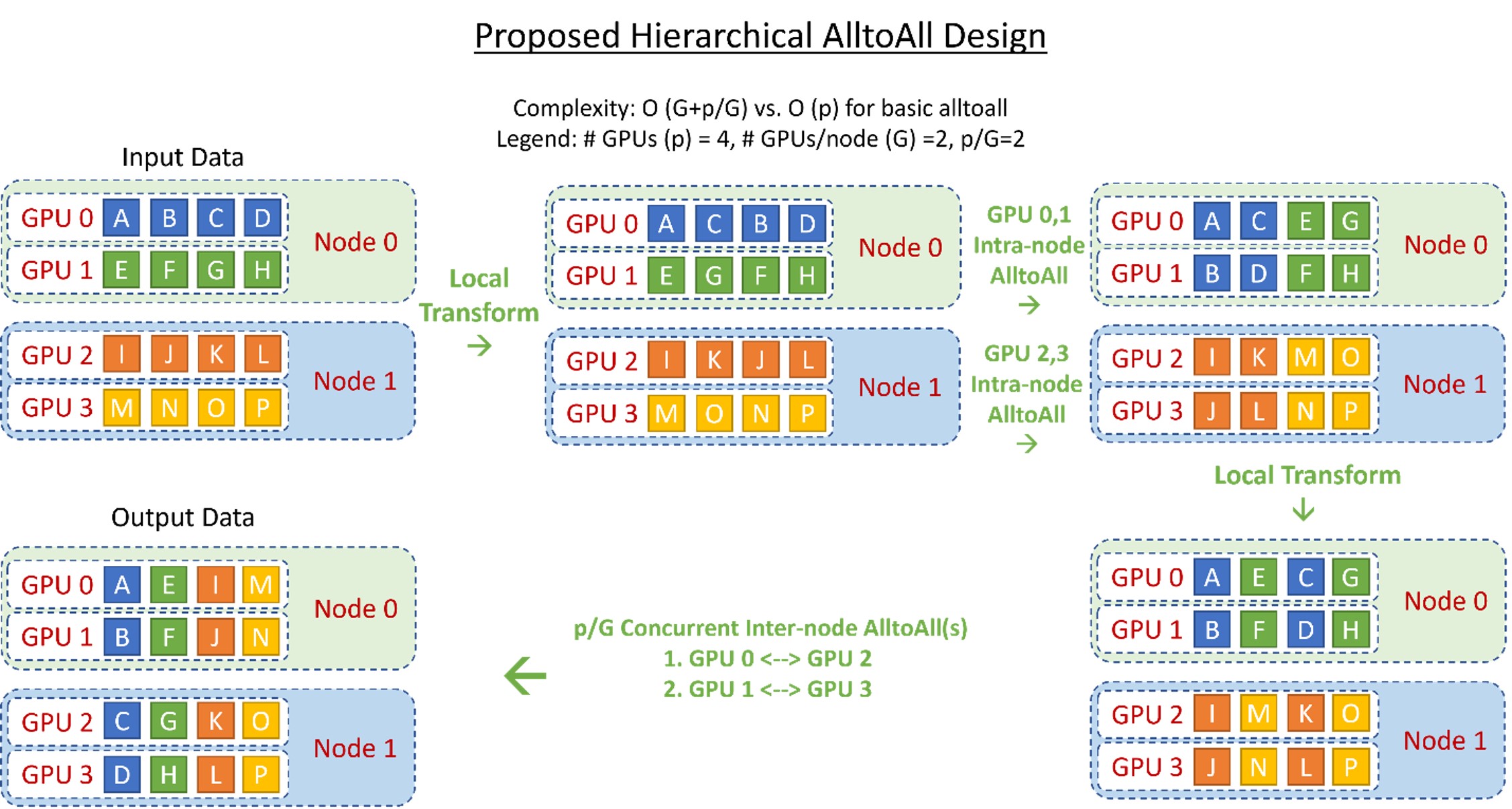
Hierarchical All-to-All: We implement a hierarchical all-to-all as a two-step process with a data-layout transformation, followed by an intra-node all-to-all, followed by a second data-layout transformation and a final inter-node all-to-all. This reduces the communication hops from O (p) to O (G+p/G), where G is the number of GPUs in a node and p is the total number of GPU devices. Figure 4 shows the design overview of this implementation. Despite the 2x increase in communication volume, this hierarchical implementation allows for better scaling for small batch sizes as communication at this message size is more latency-bound than bandwidth-bound.
Figure 4: Illustration of the proposed hierarchical all-to-all design
Parallelism Coordinated Communication Optimization: Combining expert parallelism and tensor-slicing with data parallelism within a single model is non-trivial. Tensor-slicing splits individual operators across GPUs and requires all-reduce between them, while expert parallelism places expert operators across GPUs without splitting them and requires all-to-all between them. By design, a naïve approach to handle these communication steps will be inefficient.
Figure 5: Illustration of the parallelism coordinated communication
To this end, we propose a novel design, as shown in Figure 5, that performs all-to-all only on a subset of devices that share the same tensor-slicing rank instead of all expert-parallel processes. As a result, the latency of all-to-all can be reduced to O(p/L) instead of O(p) where L is the tensor-slicing parallelism degree. This reduced latency enables us to scale inference to hundreds of GPU devices.
DS-MoE inference system consists of highly optimized kernels targeting both transformer and MoE-related operations. These kernels aim for maximizing the bandwidth utilization by fusing the operations that work in producer-consumer fashion. In addition to computation required for the transformer layers (explained in this blog post), MoE models require the following additional operations:
a gating function that determines the assignment of tokens to experts, where the result is represented as a sparse tensor.
a sparse einsum operator, between the one-hot tensor and all the tokens, which sorts the ordering of the tokens based on the assigned expert ID.
a final einsum that scales and re-sorts the tokens back to their original ordering.
The gating function includes numerous operations to create token-masks, select top-k experts, and perform cumulative-sum and sparse matrix-multiply, all of which are not only wasteful due to the sparse tenor representation, but also extremely slow due to many kernel call invocations. Moreover, the sparse einsums have a complexity of SxExMxc (number of tokens S, number of experts E, model dimension M, and expert capacity c that is typically 1), but E-1 out of E operators for each token are multiplication and addition with zeros.
We optimize these operators using dense representation and kernel-fusion. First, we fuse the gating function into a single kernel, and use a dense token-to-expert mapping table to represent the assignment from tokens to experts, greatly reducing the kernel launch overhead, as well as memory and compute overhead from the sparse representation.
Second, to optimize the remaining two sparse einsums, we implement them as data layout transformations using the above-mentioned mapping table, to first sort them based on the expert id and then back to its original ordering without requiring any sparse einsum, reducing the complexity of these operations from SxExMxc to SxMxc. Combined, these optimizations result in over 6x reduction in MoE kernel related latency.
Low latency and high throughput at unprecedented scale
In modern production environments, powerful DL models are often served using hundreds of GPU devices to meet the traffic demand and deliver low latency. Here we demonstrate the performance of DS-MoE Inference System on a 256 A100 with 40 GB GPUs. Table 3 shows various model configurations used for performance comparisons in this section.
Model
Size (billions)
# of Layers
Hidden size
Model-Parallel degree
Expert-Parallel degree
2.4B+MoE-128
107.7
16
3,584
1
128
8B+MoE-128
349.0
40
4,096
4
128
24B+MoE-128
1,046.9
30
8,192
8
128
47B+MoE-128
2,024.0
58
8,192
8
128
Table 3. The configuration of different MoE models used for the performance evaluation of Figure 6.
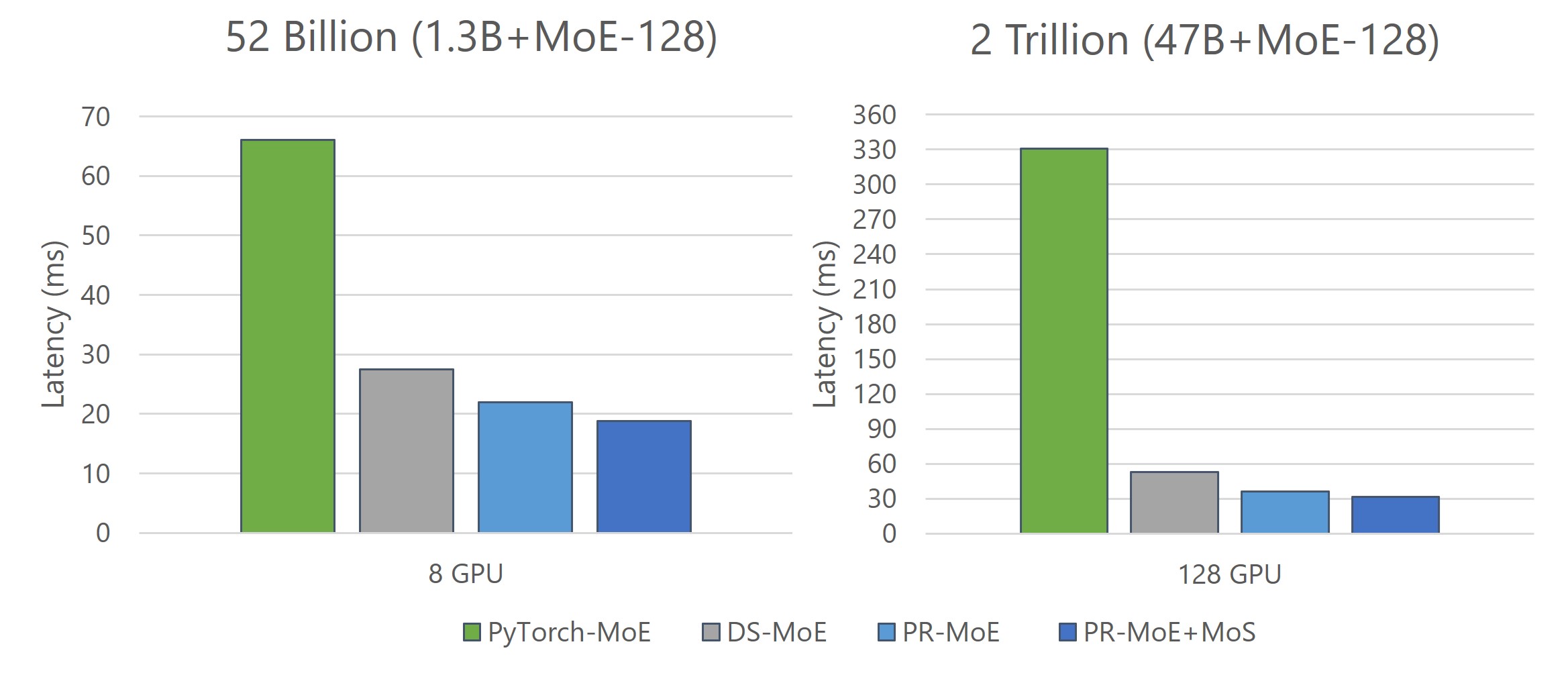
We scale MoE models from 107 billion parameters to 2 trillion parameters. To offer a strong baseline for comparison, we utilize a full-featured distributed PyTorch implementation that is capable of both tensor-slicing and expert-parallelism. Figure 6 shows the results for all these model configurations:
DeepSpeed MoE achieves up to 7.3x reduction in latency while achieving up to 7.3x higher throughput compared to the baseline.
By effectively exploiting hundreds of GPUs in parallel, DeepSpeed MoE achieves an unprecedented scale for inference at incredibly low latencies – a staggering trillion parameter MoE model can be inferenced under 25ms.
Figure 6: Latency and throughput Improvement offered by DeepSpeed-Inference-MoE (Optimized) over PyTorch (Baseline) for different model sizes (107 billion to 2 trillion parameters). We use 128 GPUs for all configurations for baseline, and 128/256 GPUs for DeepSpeed (256 GPUs for the trillion-scale models). The throughputs shown here are per GPU and should be multiplied by number of GPUs to get the aggregate throughput of the cluster.
By combining the system optimizations offered by the DS-MoE inference system and model innovations of PR-MoE and MoS, DeepSpeed MoE delivers two more benefits:
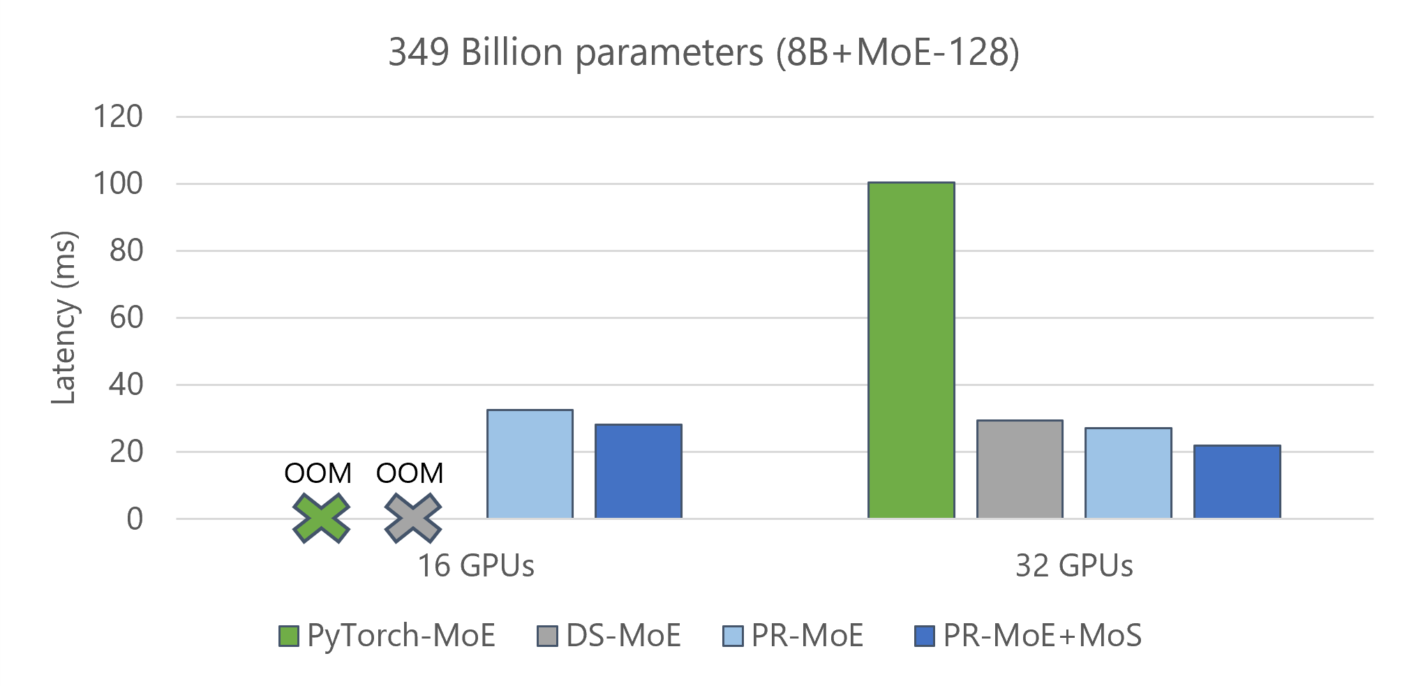
Reduce the minimum number of GPUs required to perform inference on these models. Figure 7 shows a comparison of three model variants along with the baseline: 1) standard MoE Model (8b-MoE-128), 2) PR-MoE model, and 3) PR-MoE+MoS model. The PR-MoE+MoS model performs the best as expected. The key observation is that the PR-MoE and MoS optimizations allow us to use 16 GPUs instead of 32 GPUs to perform this inference.
Further improve both latency and throughput of various MoE model sizes (as shown in Figure 8).
Figure 7: 2x fewer resources needed for MoE inference when using PR-MoE+MoS.
Figure 8: Inference latency comparing standard-MoE with PR-MoE and PR-MoE + MoS compression on different GPU count and model sizes
Better inference latency and throughput than quality-equivalent dense models
To better understand the inference performance of MoE models compared to quality-equivalent dense models, it is important to note that although MoE models are 5x faster and cheaper to train, that may not be true for inference. Inference performance has different bottlenecks and its primary factor is the amount of data read from memory instead of computation.
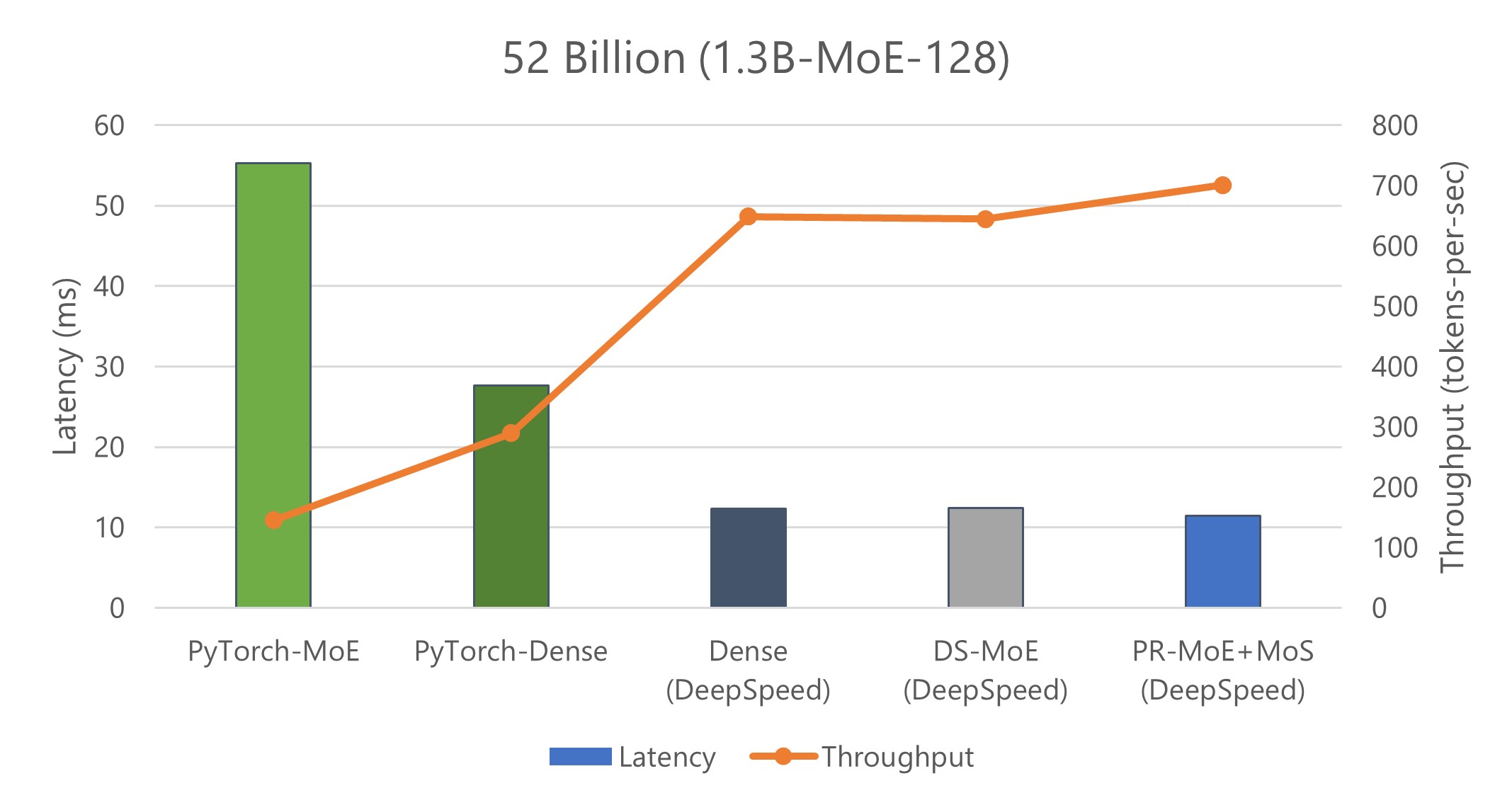
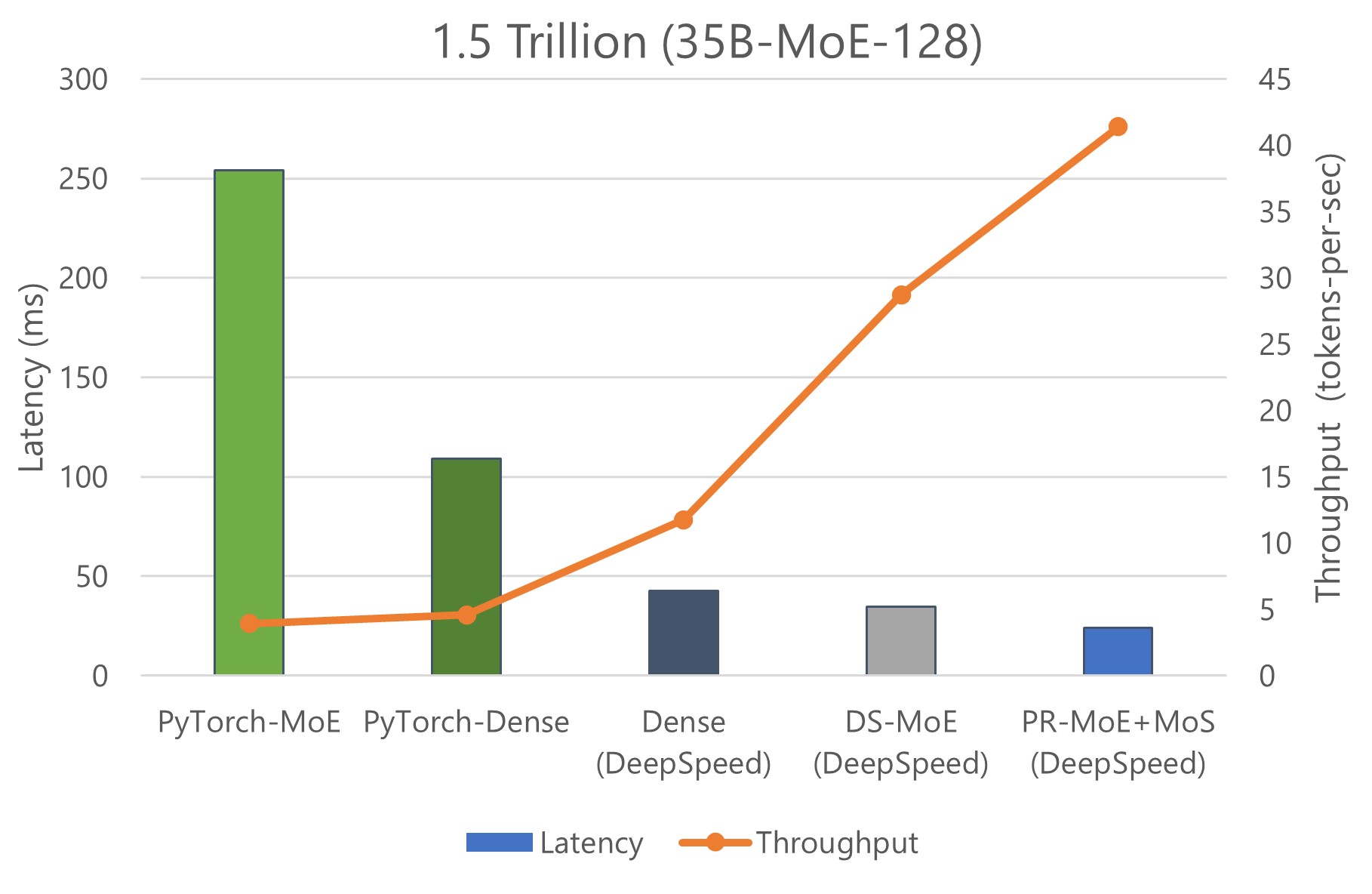
We show inference latency and throughput for two MoE models compared to their quality-equivalent dense models: a) 52 billion-parameter MoE (1.3B-MoE-128) model compared to a 6.7 billion-parameter dense model and b) 1.5 trillion-parameter MoE model compared to a 175 billion-parameter dense model in Figures 9 and 10, respectively.
When using PyTorch, MoE model inference is more expensive and slower compared to its quality-equivalent dense models. This is true for both model sizes. However, the optimizations in DS-MoE reverse this trend and make MoE model inference both faster and cheaper compared to quality-equivalent dense models. This is a critical result, showing MoE’s benefits over dense beyond training but also on inference latency and cost, which is important to real-world deployments.
When comparing the results of Figure 9 with Figure 10, we observe that the benefits of MoE models over dense models become even larger with the increase of model size. While the 52 billion-parameter MoE model is 2.4x faster and cheaper than the 6.7 billion-parameter dense model, the 1.5 trillion-parameter MoE model is 4.5x faster and 9x cheaper than the 175 billion-parameter dense model. The benefits increase for larger models because DS-MoE leverages parallelism-coordinated optimization to reduce communication overhead when using tensor-slicing on non-expert part of model. Furthermore, we can take advantage of expert-slicing at this scale, which enables us to scale to a higher number of GPUs compared to the PyTorch baseline. In addition, for the larger 1.5 trillion-parameter MoE model, we observed 2x additional improvement in throughput over latency as shown in Figure 10. This is because MoE models can run with half the tensor-slicing degree of the dense model (8-way vs. 16-way) and thus two times higher batch size.
Overall, DeepSpeed MoE delivers up to 4.5x faster and up to 9x cheaper MoE model inference compared to serving quality-equivalent dense models using PyTorch. With benefits that scale with model size and hardware resources, as shown from these results, it makes us believe that MoE models will be crucial to bring the next generation of advances in AI scale.
Figure 9: Inference latency comparison of a 52 billion-parameter MoE model and its quality-equivalent 6.7 billion-parameter dense model. We use 1 GPU for 6.7 billion-parameter model as it offers the lowest latency. We use 128 GPUs for the 52 billion-parameter model. The quality-equivalence has been verified by experiments presented in the training section.
Figure 10: Measured inference latency comparison of a 1.5 trillion-parameter MoE model and its quality-equivalent 175 billion dense model. We assume the quality equivalence of these two models with the hypothesis that the scaling law of the smaller scale experiments of Figure 9 holds, as well as from the observations of the published literature.
Looking forward to the next generation of AI Scale
With the exponential growth of model size recently, we have arrived at the boundary of what modern supercomputing clusters can do to train and serve large models. It is no longer feasible to achieve better model quality by simply increasing the model size due to insurmountable requirements on hardware resources. The choices we have are to wait for the next generation of hardware or to innovate and improve the training and inference efficiency using current hardware.
We, along with recent literature, have demonstrated how MoE-based models can reduce the training cost of even the largest NLG models by several times compared to their quality-equivalent dense counterparts, offering the possibility to train the next scale of AI models on current generation of hardware. However, prior to this blog post, to our knowledge there have been no existing works on how to serve the MoE models (with many more parameters) with latency and cost better than the dense models. This is a challenging issue that blocks practical use.
To enable practical and efficient inference for MoE models, we offer novel PR-MoE model architecture and MoS distillation technique to significantly reduce the memory requirements of these models. We also offer an MoE inference framework to achieve incredibly low latency and cost at an unprecedented model scale. Combining these innovations, we are able to make these MoE models not just feasible to serve but able to be used for inference at lower latency and cost than their quality-equivalent dense counterparts.
As a whole, the new innovations and infrastructures offer a promising path towards training and inference of the next generation of AI scale, without requiring an increase in compute resources. A shift from dense to sparse MoE models can open a path to new directions in the large model landscape, where deploying higher-quality models is widely possible with fewer resources and is more sustainable by reducing the environmental impact of large-scale AI.
Software: The best place to train and serve models using DeepSpeed is the Microsoft Azure AI platform. To get started with DeepSpeed on Azure, follow the tutorial and experiment with different models using our Azure ML examples. You can also measure your model’s energy consumption using the latest Azure Machine Learning resource metrics.
With this release of DeepSpeed, we are releasing a generic end-to-end framework for training and inference of MoE-based models. The MoE training support and optimizations are made available in full. The MoE inference optimizations will be released in two phases. The generic flexible parallelism framework for MoE inference is being released today. Optimizations related to computation kernels and communication will be released in future.
DeepSpeed is a deep learning optimization library that makes distributed training easy, efficient, and effective.
To enable experimentation with DeepSpeed MoE optimizations, we are also releasing two extensions of the NLG example that enables 5x reduction in training cost for MT-NLG like models: 1) PR-MoE model extension to enable 3x improvement in parameter efficiency and model size reduction and 2) Model code extensions so users can easily experiment with MoE inference at scale. Please find the code, tutorials, and documents at DeepSpeed GitHub and website.
About our great collaborators
This work was done in collaboration with Brandon Norick, Zhun Liu, and Xia Song from the Turing Team, Young Jin Kim, Alex Muzio, and Hany Hassan Awadalla from the Z-Code Team, and both Saeed Maleki and Madan Musuvathi from the SCCL team.
About the DeepSpeed Team
We are a group of system researchers and engineers—Samyam Rajbhandari, Ammar Ahmad Awan, Jeff Rasley, Reza Yazdani Aminabadi, Minjia Zhang, Zhewei Yao, Conglong Li, Olatunji Ruwase, Elton Zheng, Shaden Smith, Cheng Li, Du Li, Yang Li, Xiaoxia Wu, Jeffery Zhu (PM), Yuxiong He (team lead)—who are enthusiastic about performance optimization of large-scale systems. We have recently focused on deep learning systems, optimizing deep learning’s speed to train, speed to convergence, and speed to develop! If this type of work interests you, the DeepSpeed team is hiring both researchers and engineers! Please visit our careers page.
With a new year underway, NVIDIA is helping enterprises worldwide add modern workloads to their mainstream servers using the latest release of the NVIDIA AI Enterprise software suite.
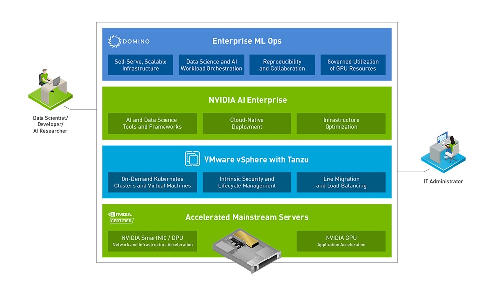
NVIDIA AI Enterprise 1.1 is now generally available. Optimized, certified and supported by NVIDIA, the latest version of the software suite brings new updates including production support for containerized AI with the NVIDIA software on VMware vSphere with Tanzu, which was previously only available on a trial basis. Now, enterprises can run accelerated AI workloads on vSphere, running in both Kubernetes containers and virtual machines with NVIDIA AI Enterprise to support advanced AI development on mainstream IT infrastructure.
Enterprise AI Simplified with VMware vSphere with Tanzu, Coming Soon to NVIDIA LaunchPad
Among the top customer-requested features in NVIDIA AI Enterprise 1.1 is production support for running on VMware vSphere with Tanzu, which enables developers to run AI workloads on both containers and virtual machines within their vSphere environments. This new milestone in the AI-ready platform curated by NVIDIA and VMware provides an integrated, complete stack of containerized software and hardware optimized for AI, all fully managed by IT.
NVIDIA will soon add VMware vSphere with Tanzu support to the NVIDIA LaunchPad program for NVIDIA AI Enterprise, available at nine Equinix locations around the world. Qualified enterprises can test and prototype AI workloads at no charge through curated labs designed for the AI practitioner and IT admin. The labs showcase how to develop and manage common AI workloads like chatbots and recommendation systems, using NVIDIA AI Enterprise and VMware vSphere, and soon with Tanzu.
“Organizations are accelerating AI and ML development projects and VMware vSphere with Tanzu running NVIDIA AI Enterprise easily empowers AI development requirements with modern infrastructure services,” said Matt Morgan, vice president of Product Marketing, Cloud Infrastructure Business Group at VMware. “This announcement marks another key milestone for VMware and NVIDIA in our sustained efforts to help teams leverage AI across the enterprise.”
Growing Demand for Containerized AI Development
While enterprises are eager to use containerized development for AI, the complexity of these workloads requires orchestration across many layers of infrastructure. NVIDIA AI Enterprise 1.1 provides an ideal solution for these challenges as an AI-ready enterprise platform.
“AI is a very popular modern workload that is increasingly favoring deployment in containers. However, deploying AI capabilities at scale within the enterprise can be extremely complex, requiring enablement at multiple layers of the stack, from AI software frameworks, operating systems, containers, VMs, and down to the hardware,” said Gary Chen, research director, Software Defined Compute at IDC. “Turnkey, full-stack AI solutions can greatly simplify deployment and make AI more accessible within the enterprise.”
Domino Data Lab MLOps Validation Accelerates AI Research and Data Science Lifecycle
The 1.1 release of NVIDIA AI Enterprise also provides validation for the Domino Data Lab Enterprise MLOps Platform with VMware vSphere with Tanzu. This new integration enables more companies to cost-effectively scale data science by accelerating research, model development, and model deployment on mainstream accelerated servers.
“This new phase of our collaboration with NVIDIA further enables enterprises to solve the world’s most challenging problems by putting models at the heart of their businesses,” said Thomas Robinson, vice president of Strategic Partnerships at Domino Data Lab. “Together, we are providing every company the end-to-end platform to rapidly and cost-effectively deploy models enterprise-wide.”
NVIDIA AI Enterprise 1.1 features support for VMware vSphere with Tanzu and validation for the Domino Data Lab Enterprise MLOps Platform.
New OEMs and Integrators Offering NVIDIA-Certified Systems for NVIDIA AI Enterprise
Amidst the new release of NVIDIA AI Enterprise, the industry ecosystem is expanding with the first NVIDIA-Certified Systems from Cisco and Hitachi Vantara, as well as a growing roster of newly qualified system integrators offering solutions for the software suite.
The first Cisco system to be NVIDIA-Certified for NVIDIA AI Enterprise is the Cisco UCS C240 M6 rack server with NVIDIA A100 Tensor Core GPUs. The two-socket, 2RU form factor can power a wide range of storage and I/O-intensive applications, such as big data analytics, databases, collaboration, virtualization, consolidation and high-performance computing.
“At Cisco we are helping simplify customers’ hybrid cloud and cloud-native transformation. NVIDIA-Certified Cisco UCS servers, powered by Cisco Intersight, deliver the best-in-class AI workload experiences in the market,” said Siva Sivakumar, vice president of product management at Cisco. “The certification of the Cisco UCS C240 M6 rack server for NVIDIA AI Enterprise allows customers to add AI using the same infrastructure and management software deployed throughout their data center.”
The first NVIDIA-Certified System from Hitachi Vantara compatible with NVIDIA AI Enterprise is the Hitachi Advanced Server DS220 G2 with NVIDIA A100 Tensor Core GPUs. The general-purpose, dual-processor server is optimized for performance and capacity, and delivers a balance of compute and storage with the flexibility to power a wide range of solutions and applications.
“For many enterprises, cost is an important consideration when deploying new technologies like AI-powered quality control, recommender systems, chatbots and more,” said Dan McConnell, senior vice president, Product Management at Hitachi Vantara. “Accelerated with NVIDIA A100 GPUs and now certified for NVIDIA AI Enterprise, Hitachi Unified Compute Platform (UCP) solutions using the Hitachi Advanced Server DS220 G2 gives customers an ideal path for affordably integrating powerful AI-ready infrastructure to their data centers.”
A broad range of additional server manufacturers offer NVIDIA-Certified Systems for NVIDIA AI Enterprise. These include Atos, Dell Technologies, GIGABYTE, H3C, Hewlett Packard Enterprise, Inspur, Lenovo and Supermicro, all of whose systems feature NVIDIA A100, NVIDIA A30 or other NVIDIA GPUs. Customers can also choose to deploy NVIDIA AI Enterprise on their own servers or on as-a-service bare metal infrastructure from Equinix Metal across nine regions globally.
AMAX, Colfax International, Exxact Corporation and Lambda are the newest system integrators qualified for NVIDIA AI Enterprise, joining a global ecosystem of channel partners that includes Axians, Carahsoft Technology Corp., Computacenter, Insight Enterprises, NTT, Presidio, Sirius, SoftServe, SVA System Vertrieb Alexander GmbH, TD SYNNEX, Trace3 and World Wide Technology.
Browse through MORF Gallery — virtually or at an in-person exhibition — and you’ll find robots that paint, digital dreamscape experiences, and fine art brought to life by visual effects.
The gallery showcases cutting-edge, one-of-a-kind artwork from award-winning artists who fuse their creative skills with AI, machine learning, robotics and neuroscience.
Scott Birnbaum, CEO and co-founder of MORF Gallery, a Silicon Valley startup, spoke with NVIDIA AI Podcast host Noah Kravitz about digital art, non-fungible tokens, as well as ArtStick, a plug-in device that turns any TV into a premium digital art gallery.
Artists featured by MORF Gallery create fine art using cutting-edge technology. For example, robots help with mundane tasks like painting backgrounds. Visual effects add movement to still paintings. And machine learning can help make NeoMasters — paintings based on original works that were once lost but resurrected or recreated with AI’s help.
The digital art space offers new and expanding opportunities for artists, technologists, collectors and investors. For one, non-fungible tokens, Birnbaum says, have been gaining lots of attention recently. He gives an overview of NFTs and how they authenticate original pieces of digital art.
Tweetables:
Paintbrushes, cameras, computers and AI are all technologies that “move the art world forward … as extensions of human creativity.” — Scott Birnbaum [8:27]
“Technology is enabling creative artists to really push the boundaries of what their imaginations can allow.” — Scott Birnbaum [13:33]
Pindar Van Arman, an American artist and roboticist, designs painting robots that explore the differences between human and computational creativity. Since his first system in 2005, he has built multiple artificially creative robots. The most famous, Cloud Painter, was awarded first place at Robotart 2018.
Steven Frank is a partner at the law firm Morgan Lewis, specializing in intellectual property and commercial technology law. He’s also half of the husband-wife team that used convolutional neural networks to authenticate artistic masterpieces, including Da Vinci’s Salvador Mundi, with AI’s help.
Researchers in the Department of Anthropology at Northern Arizona University are using GPU-based deep learning algorithms to categorize sherds — tiny fragments of ancient pottery.
In a busy hospital, a radiologist is using an artificial intelligence system to help her diagnose medical conditions based on patients’ X-ray images. Using the AI system can help her make faster diagnoses, but how does she know when to trust the AI’s predictions?
She doesn’t. Instead, she may rely on her expertise, a confidence level provided by the system itself, or an explanation of how the algorithm made its prediction — which may look convincing but still be wrong — to make an estimation.
To help people better understand when to trust an AI “teammate,” MIT researchers created an onboarding technique that guides humans to develop a more accurate understanding of those situations in which a machine makes correct predictions and those in which it makes incorrect predictions.
By showing people how the AI complements their abilities, the training technique could help humans make better decisions or come to conclusions faster when working with AI agents.
“We propose a teaching phase where we gradually introduce the human to this AI model so they can, for themselves, see its weaknesses and strengths,” says Hussein Mozannar, a graduate student in the Social and Engineering Systems doctoral program within the Institute for Data, Systems, and Society (IDSS) who is also a researcher with the Clinical Machine Learning Group of the Computer Science and Artificial Intelligence Laboratory (CSAIL) and the Institute for Medical Engineering and Science. “We do this by mimicking the way the human will interact with the AI in practice, but we intervene to give them feedback to help them understand each interaction they are making with the AI.”
Mozannar wrote the paper with Arvind Satyanarayan, an assistant professor of computer science who leads the Visualization Group in CSAIL; and senior author David Sontag, an associate professor of electrical engineering and computer science at MIT and leader of the Clinical Machine Learning Group. The research will be presented at the Association for the Advancement of Artificial Intelligence in February.
Mental models
This work focuses on the mental models humans build about others. If the radiologist is not sure about a case, she may ask a colleague who is an expert in a certain area. From past experience and her knowledge of this colleague, she has a mental model of his strengths and weaknesses that she uses to assess his advice.
Humans build the same kinds of mental models when they interact with AI agents, so it is important those models are accurate, Mozannar says. Cognitive science suggests that humans make decisions for complex tasks by remembering past interactions and experiences. So, the researchers designed an onboarding process that provides representative examples of the human and AI working together, which serve as reference points the human can draw on in the future. They began by creating an algorithm that can identify examples that will best teach the human about the AI.
“We first learn a human expert’s biases and strengths, using observations of their past decisions unguided by AI,” Mozannar says. “We combine our knowledge about the human with what we know about the AI to see where it will be helpful for the human to rely on the AI. Then we obtain cases where we know the human should rely on the AI and similar cases where the human should not rely on the AI.”
The researchers tested their onboarding technique on a passage-based question answering task: The user receives a written passage and a question whose answer is contained in the passage. The user then has to answer the question and can click a button to “let the AI answer.” The user can’t see the AI answer in advance, however, requiring them to rely on their mental model of the AI. The onboarding process they developed begins by showing these examples to the user, who tries to make a prediction with the help of the AI system. The human may be right or wrong, and the AI may be right or wrong, but in either case, after solving the example, the user sees the correct answer and an explanation for why the AI chose its prediction. To help the user generalize from the example, two contrasting examples are shown that explain why the AI got it right or wrong.
For instance, perhaps the training question asks which of two plants is native to more continents, based on a convoluted paragraph from a botany textbook. The human can answer on her own or let the AI system answer. Then, she sees two follow-up examples that help her get a better sense of the AI’s abilities. Perhaps the AI is wrong on a follow-up question about fruits but right on a question about geology. In each example, the words the system used to make its prediction are highlighted. Seeing the highlighted words helps the human understand the limits of the AI agent, explains Mozannar.
To help the user retain what they have learned, the user then writes down the rule she infers from this teaching example, such as “This AI is not good at predicting flowers.” She can then refer to these rules later when working with the agent in practice. These rules also constitute a formalization of the user’s mental model of the AI.
The impact of teaching
The researchers tested this teaching technique with three groups of participants. One group went through the entire onboarding technique, another group did not receive the follow-up comparison examples, and the baseline group didn’t receive any teaching but could see the AI’s answer in advance.
“The participants who received teaching did just as well as the participants who didn’t receive teaching but could see the AI’s answer. So, the conclusion there is they are able to simulate the AI’s answer as well as if they had seen it,” Mozannar says.
The researchers dug deeper into the data to see the rules individual participants wrote. They found that almost 50 percent of the people who received training wrote accurate lessons of the AI’s abilities. Those who had accurate lessons were right on 63 percent of the examples, whereas those who didn’t have accurate lessons were right on 54 percent. And those who didn’t receive teaching but could see the AI answers were right on 57 percent of the questions.
“When teaching is successful, it has a significant impact. That is the takeaway here. When we are able to teach participants effectively, they are able to do better than if you actually gave them the answer,” he says.
But the results also show there is still a gap. Only 50 percent of those who were trained built accurate mental models of the AI, and even those who did were only right 63 percent of the time. Even though they learned accurate lessons, they didn’t always follow their own rules, Mozannar says.
That is one question that leaves the researchers scratching their heads — even if people know the AI should be right, why won’t they listen to their own mental model? They want to explore this question in the future, as well as refine the onboarding process to reduce the amount of time it takes. They are also interested in running user studies with more complex AI models, particularly in health care settings.
“When humans collaborate with other humans, we rely heavily on knowing what our collaborators’ strengths and weaknesses are — it helps us know when (and when not) to lean on the other person for assistance. I’m glad to see this research applying that principle to humans and AI,” says Carrie Cai, a staff research scientist in the People + AI Research and Responsible AI groups at Google, who was not involved with this research. “Teaching users about an AI’s strengths and weaknesses is essential to producing positive human-AI joint outcomes.”
This research was supported, in part, by the National Science Foundation.
Natural language understanding is applied in a wide range of use cases, from chatbots and virtual assistants, to machine translation and text summarization. To ensure that these applications are running at an expected level of performance, it’s important that data in the training and production environments is from the same distribution. When the data that is used for inference (production data) differs from the data used during model training, we encounter a phenomenon known as data drift. When data drift occurs, the model is no longer relevant to the data in production and likely performs worse than expected. It’s important to continuously monitor the inference data and compare it to the data used during training.
You can use Amazon SageMaker to quickly build, train, and deploy machine learning (ML) models at any scale. As a proactive measure against model degradation, you can use Amazon SageMaker Model Monitor to continuously monitor the quality of your ML models in real time. With Model Monitor, you can also configure alerts to notify and trigger actions if any drift in model performance is observed. Early and proactive detection of these deviations enables you to take corrective actions, such as collecting new ground truth training data, retraining models, and auditing upstream systems, without having to manually monitor models or build additional tooling.
Model Monitor offers four different types of monitoring capabilities to detect and mitigate model drift in real time:
Data quality – Helps detect change in data schemas and statistical properties of independent variables and alerts when a drift is detected.
Model quality – For monitoring model performance characteristics such as accuracy or precision in real time, Model Monitor allows you to ingest the ground truth labels collected from your applications. Model Monitor automatically merges the ground truth information with prediction data to compute the model performance metrics.
Model bias –Model Monitor is integrated with Amazon SageMaker Clarify to improve visibility into potential bias. Although your initial data or model may not be biased, changes in the world may cause bias to develop over time in a model that has already been trained.
Model explainability – Drift detection alerts you when a change occurs in the relative importance of feature attributions.
In this post, we discuss the types of data quality drift that are applicable to text data. We also present an approach to detecting data drift in text data using Model Monitor.
Data drift in NLP
Data drift can be classified into three categories depending on whether the distribution shift is happening on the input or on the output side, or whether the relationship between the input and the output has changed.
Covariate shift
In a covariate shift, the distribution of inputs changes over time, but the conditional distribution P(y|x) doesn’t change. This type of drift is called covariate shift because the problem arises due to a shift in the distribution of the covariates (features). For example, in an email spam classification model, distribution of training data (email corpora) may diverge from the distribution of data during scoring.
Label shift
While covariate shift focuses on changes in the feature distribution, label shift focuses on changes in the distribution of the class variable. This type of shifting is essentially the reverse of covariate shift. An intuitive way to think about it might be to consider an unbalanced dataset. If the spam to non-spam ratio of emails in our training set is 50%, but in reality 10% of our emails are non-spam, then the target label distribution has shifted.
Concept shift
Concept shift is different from covariate and label shift in that it’s not related to the data distribution or the class distribution, but instead is related to the relationship between the two variables. For example, email spammers often use a variety of concepts to pass the spam filter models, and the concept of emails used during training may change as time goes by.
Now that we understand the different types of data drift, let’s see how we can use Model Monitor to detect covariate shift in text data.
Solution overview
Unlike tabular data, which is structured and bounded, textual data is complex, high dimensional, and free form. To efficiently detect drift in NLP, we work with embeddings, which are low-dimensional representations of the text. You can obtain embeddings using various language models such as Word2Vec and transformer-based models like BERT. These models project high-dimensional data into low-dimensional spaces while preserving the semantic information of the text. The results are dense and contextually meaningful vectors, which can be used for various downstream tasks, including monitoring for data drift.
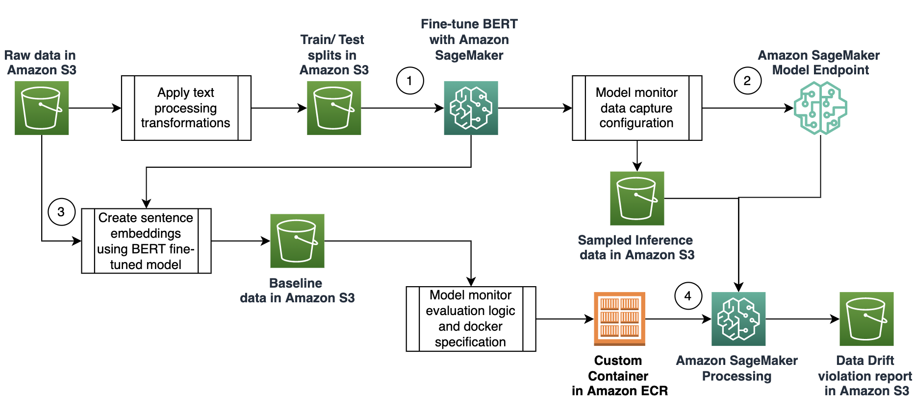
In our solution, we use embeddings to detect the covariate shift of English sentences. We utilize Model Monitor to facilitate continuous monitoring for a text classifier that is deployed to a production environment. Our approach consists of the following steps:
Fine-tune a BERT model using SageMaker.
Deploy a fine-tuned BERT classifier as a real-time endpoint with data capture enabled.
Create a baseline dataset that consists of a sample of the sentences used to train the BERT classifier.
Create a custom SageMaker monitoring job to calculate the cosine similarity between the data captured in production and the baseline dataset.
The following diagram illustrates the solution workflow:
Fine-tune a BERT model
In this post, we use Corpus of Linguistic Acceptability (CoLA), a dataset of 10,657 English sentences labeled as grammatical or ungrammatical from published linguistics literature. We use SageMaker training to fine-tune a BERT model using the CoLa dataset by defining an PyTorch estimator class. For more information on how to use this SDK with PyTorch, see Use PyTorch with the SageMaker Python SDK. Calling the fit() method of the estimator launches the training job:
from sagemaker.pytorch import PyTorch

# place to save model artifact
output_path = f"s3://{bucket}/{model_prefix}"

estimator = PyTorch(
    entry_point="train_deploy.py",
    source_dir="code",
    role=role,
    framework_version="1.7.1",
    py_version="py3",
    instance_count=1,
    instance_type="ml.p3.2xlarge",
    output_path=output_path,
    hyperparameters={
        "epochs": 1,
        "num_labels": 2,
        "backend": "gloo",
    },
    disable_profiler=True, # disable debugger
)
estimator.fit({"training": inputs_train, "testing": inputs_test})
Deploy the model
After training our model, we host it on a SageMaker endpoint. To make the endpoint load the model and serve predictions, we implement a few methods in train_deploy.py:
model_fn() – Loads the saved model and returns a model object that can be used for model serving. The SageMaker PyTorch model server loads our model by invoking model_fn.
input_fn() – Deserializes and prepares the prediction input. In this example, our request body is first serialized to JSON and then sent to the model serving endpoint. Therefore, in input_fn(), we first deserialize the JSON-formatted request body and return the input as a torch.tensor, as required for BERT.
predict_fn() – Performs the prediction and returns the result.
We run prediction using the predictor object that we created in the previous step. We set JSON serializer and deserializer, which is used by the inference endpoint:
print("Sending test traffic to the endpoint {}. nPlease wait...".format(endpoint_name))

result = predictor.predict([
"Thanks so much for driving me home",
"Thanks so much for cooking dinner. I really appreciate it",
"Nice to meet you, Sergio. So, where are you from"
])
The real-time endpoint is configured to capture data from the request, and the response and the data gets stored in Amazon S3. You can view the data that’s captured in the previous monitoring schedule.
Create a baseline
We use a fine-tuned BERT model to extract sentence embedding features from the training data. We use these vectors as high-quality feature inputs for comparing cosine distance because BERT produces dynamic word representation with semantic context. Complete the following steps to get sentence embedding:
Use a BERT tokenizer to get token IDs for each token (input_id) in the input sentence and mask to indicate which elements in the input sequence are tokens vs. padding elements (attention_mask_id). We use the BERT tokenizer.encode_plus function to get these values for each input sentence:
#Add instantiation of tokenizer
encoded_dict = tokenizer.encode_plus(
               sent,                      # Input Sentence to encode.
               add_special_tokens = True, # Add '[CLS]' and '[SEP]'
               max_length = 64,           # Pad sentence to max_length
               pad_to_max_length = True,  # Truncate sentence to max_length
               return_attention_mask = True, #BERT model needs attention_mask
               return_tensors = 'pt',     # Return pytorch tensors.
               )
input_ids = encoded_dict['input_ids']
attention_mask_ids = encoded_dict['attention_mask']
input_ids and attention_mask_ids are passed to the model and fetch the hidden states of the network. The hidden_states has four dimensions in the following order:
Layer number (BERT has 12 layers)
Batch number (1 sentence)
Word token indexes
Hidden units (768 features)
Use the last two hidden layers to get a single vector (sentence embedding) by calculating the average of all input tokens in the sentence:
outputs = model(input_ids, attention_mask_ids) # forward pass to model
hidden_states = outputs[2]                     # token vectors
token_vecs = hidden_states[-2][0]              # last 2 layer hidden states
sentence_embedding = torch.mean(token_vecs, dim=0) # average token vectors
Convert the sentence embedding as a NumPy array and store it in an Amazon S3 location as a baseline that is used by Model Monitor:
sentence_embeddings_list = []for i in sentence_embeddings:sentence_embeddings_list.append(i.numpy())

np.save('embeddings.npy', sentence_embeddings_list)

#Upload the sentence embedding to S3
!aws s3 cp embeddings.npy s3://{bucket}/{model_prefix}/embeddings/
Evaluation script
Model Monitor provides a pre-built container with the ability to analyze the data captured from endpoints for tabular datasets. If you want to bring your own container, Model Monitor provides extension points that you can use. When you create a MonitoringSchedule, Model Monitor ultimately kicks off processing jobs. Therefore, the container needs to be aware of the processing job contract. We need to create an evaluation script that is compatible with container contract inputs and outputs.
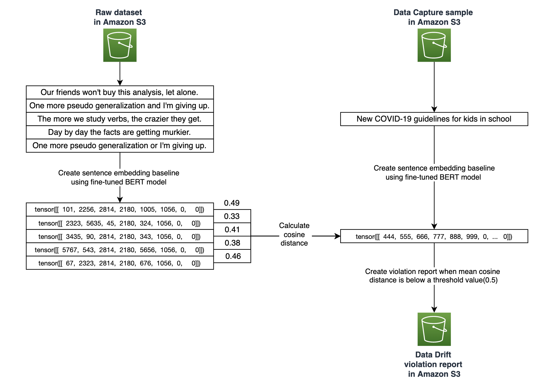
Model Monitor uses evaluation code on all the samples that are captured during the monitoring schedule. For each inference data point, we calculate the sentence embedding using the same logic described earlier. Cosine similarity is used as a distance metric to measure the similarity of an inference data point and sentence embeddings in the baseline. Mathematically, it measures the cosine angle between two sentence embedding vectors. A high the cosine similarity score indicates similar sentence embeddings. A lower cosine similarity score indicates data drift. We calculate an average of all the cosine similarity scores, and if it’s less than the threshold, it gets captured in the violation report. Based on the use case, you can use other distance metrics like manhattan or euclidean to measure similarity of sentence embeddings.
The following diagram shows how we use SageMaker Model Monitoring to establish baseline and detect data drift using cosine distance similarity.
The following is the code for calculating the violations; the complete evaluation script is available on GitHub:
for embed_item in embedding_list: # all sentence embeddings from baseline
    cosine_score += (1 - cosine(input_sentence_embedding, embed_item)) # cosine distance between input sentence embedding and baseline embedding
cosine_score_avg = cosine_score/(len(embedding_list)) # average cosine score of input sentence
if cosine_score_avg < env.max_ratio_threshold: # compare averge cosine score against a threshold
    sent_cosine_dict[record] = cosine_score_avg # capture details for violation report
    violations.append({
            "sentence": record,
            "avg_cosine_score": cosine_score_avg,
            "feature_name": "sent_cosine_score",
            "constraint_check_type": "baseline_drift_check",
            "endpoint_name" : env.sagemaker_endpoint_name,
            "monitoring_schedule_name": env.sagemaker_monitoring_schedule_name
        })
Measure data drift using Model Monitor
In this section, we focus on measuring data drift using Model Monitor. Model Monitor pre-built monitors are powered by Deequ, which is a library built on top of Apache Spark for defining unit tests for data, which measure data quality in large datasets. You don’t require coding to utilize these pre-built monitoring capabilities. You also have the flexibility to monitor models by coding to provide custom analysis. You can collect and review all metrics emitted by Model Monitor in Amazon SageMaker Studio, so you can visually analyze your model performance without writing additional code.
In certain scenarios, for instance when the data is non-tabular, the default processing job (powered by Deequ) doesn’t suffice because it only supports tabular datasets. The pre-built monitors may not be sufficient to generate sophisticated metrics to detect drifts, and may necessitate bringing your own metrics. In the next sections, we describe the setup to bring in your metrics by building a custom container.
#Build a docker container and push to ECR

account_id = boto3.client('sts').get_caller_identity().get('Account')
ecr_repository = 'nlp-data-drift-bert-v1'
tag = ':latest'
region = boto3.session.Session().region_name
sm = boto3.client('sagemaker')
uri_suffix = 'amazonaws.com'
if region in ['cn-north-1', 'cn-northwest-1']:
    uri_suffix = 'amazonaws.com.cn'
    processing_repository_uri = f'{account_id}.dkr.ecr.{region}.{uri_suffix}/{ecr_repository + tag}'
# Creating the ECR repository and pushing the container image

!docker build -t $ecr_repository docker

!$(aws ecr get-login --region $region --registry-ids $account_id --no-include-email)

!aws ecr create-repository --repository-name $ecr_repository

!docker tag {ecr_repository + tag} $processing_repository_uri!docker push $processing_repository_uri
When the customer Docker container is in Amazon ECR, we can schedule a Model Monitoring job and generate a violations report, as demonstrated in the next sections.
Schedule a model monitoring job
To schedule a model monitoring job, we create an instance of Model Monitor and in the image_uri, we refer to the Docker container that we created in the previous section:
We schedule the monitoring job using the create_monitoring_scheduleAPI. You can schedule the monitoring job on an hourly or daily basis. You configure the job using the destination parameter, as shown in the following code:
When the model monitoring job is complete, you can navigate to the destination S3 path to access the violation reports. This report contains all the inputs whose average cosine score (avg_cosine_score) is below the threshold configured as an environment variable THRESHOLD:0.5 in the ModelMonitor instance. This is an indication that the data observed during inference is drifting beyond the established baseline.
The following code shows the generated violation report:
{
    "violations": [
        {
            "feature_name": "sent_cosine_score",
            "constraint_check_type": "baseline_drift_check",
            "sentence": "Thanks so much for driving me home",
            "avg_cosine_score": 0.36653404209142876
        },
        {
            "feature_name": "sent_cosine_score",
            "constraint_check_type": "baseline_drift_check",
            "sentence": "Thanks so much for cooking dinner. I really appreciate it",
            "avg_cosine_score": 0.34974955975723576
        },
        {
            "feature_name": "sent_cosine_score",
            "constraint_check_type": "baseline_drift_check",
            "sentence": "Nice to meet you, Sergio. So, where are you from",
            "avg_cosine_score": 0.378982806084463
        }
    ]
}
Finally, based on this observation, you can configure your model for retraining. You can also enable Amazon Simple Notification Service (Amazon SNS) notifications to send alerts when violations occur.
Conclusion
Model Monitor enables you to maintain the high quality of your models in production. In this post, we highlighted the challenges with monitoring data drift on unstructured data like text, and provided an intuitive approach to detect data drift using a custom monitoring script. You can find the code associated with the post in the following GitHub repository. Additionally, you can customize the solution to utilize other distance metrics such as maximum mean discrepancy (MMD), a non-parametric distance metric to compute marginal distribution between source and target distribution on the embedded space.
About the Authors
Vikram Elango is an AI/ML Specialist Solutions Architect at Amazon Web Services, based in Virginia, USA. Vikram helps financial and insurance industry customers with design, thought leadership to build and deploy machine learning applications at scale. He is currently focused on natural language processing, responsible AI, inference optimization and scaling ML across the enterprise. In his spare time, he enjoys traveling, hiking, cooking and camping with his family.
Raghu Ramesha is a ML Solutions Architect with the Amazon SageMaker Service team. He focuses on helping customers migrate ML production workloads to SageMaker at scale. He specializes in machine learning, AI, and computer vision domains, and holds a master’s degree in Computer Science from UT Dallas. In his free time, he enjoys traveling and photography.
Tony Chen is a Machine Learning Solutions Architect at Amazon Web Services, helping customers design scalable and robust machine learning capabilities in the cloud. As a former data scientist and data engineer, he leverages his experience to help tackle some of the most challenging problems organizations face with operationalizing machine learning.

 NVIDIA GeForce NOW (@NVIDIAGFN)