Why Spectral Normalization Stabilizes GANs: Analysis and Improvements

Figure 1: Training instability is one of the biggest challenges in training GANs. Despite the existence of successful heuristics like Spectral Normalization (SN) for improving stability, it is poorly-understood why they work. In our research, we theoretically explain why SN stabilizes GAN training. Using these insights, we further propose a better normalization technique for improving GANs’ stability called Bidirectional Scaled Spectral Normalization.

Generative adversarial networks (GANs) are a class of popular generative models enabling many cutting-edge applications such as photorealistic image synthesis. Despite their tremendous success, GANs are notoriously unstable to train—small hyper-parameter changes and even randomness in optimization can cause training to fail altogether, which leads to poor generated samples. One empirical heuristic that is widely used to stabilize GAN training is spectral normalization (SN) (Figure 2). Although it is very widely adopted, little is understood about why it works, and therefore there is little analytical basis for using it, configuring it, and more importantly, improving it.

Figure 2: Spectral normalization divides the weights (W_i) by their spectral norms (sigma(W_i)) (i.e., the largest singular value of (W_i)).

In this post, we discuss our recent work at NeurIPS 2021. We prove that spectral normalization controls two well-known failure modes of training stability: exploding and vanishing gradients. More interestingly, we uncover a surprising connection between spectral normalization and neural network initialization techniques, which not only help explain how spectral normalization stabilizes GANs, but also motivate us to design Bidirectional Scaled Spectral Normalization (BSSN), a simple change to spectral normalization that yields better stability than SN (Figure 3). 

Figure 3: The interesting connections we find between spectral normalization and prior initialization techniques: (1) LeCun initialization can help explain why spectral normalization avoids vanishing gradients; (2) Motivated by newer initialization techniques (Xavier and Kaiming), we propose BSSN to further improve spectral normalization.

Exploding and vanishing gradients cause training instability

Exploding and vanishing gradients describe a problem in which gradients either grow or shrink rapidly during training. It is known in the community that these phenomena are closely related to the instability of GANs. Figure 4 shows an illustrating example: when exploding and vanishing gradients happen, the sample quality measured by inception score (higher is better) deteriorates rapidly.

Figure 4: The close connection between gradient scales and training instability. Left: the gradient norm during the training of three GANs on CIFAR-10, either with exploding, vanishing, or stable gradients. Right: the inception score (measuring sample quality; the higher, the better) of these three GANs. We see that the GANs with bad gradient scales (exploding or vanishing) have worse sample quality as measured by inception score.

In the next section, we will show how spectral normalization alleviates exploding and vanishing gradients, which may explain its success.

How spectral normalization mitigates exploding gradients

The fact that spectral normalization prevents gradient explosion is not too surprising. Intuitively, it achieves this by limiting the ability of weight tensors to amplify inputs in any direction. More precisely, when the spectral norm of weights = 1 (as ensured by spectral normalization), and the activation functions are 1-Lipschitz (e.g., (Leaky)ReLU), we show that

$$ | text{gradient} |_{text{Frobenius}} leq sqrt{text{number of layers}} cdot | text{input} |.$$

(Please refer to the paper for more general results.) In other words, the gradient norm of spectrally normalized GANs cannot exceed a strict bound. This explains why spectral normalization can mitigate exploding gradients. 

Note that this good property is not unique to spectral normalization—our analysis can also be used to show the same result for other normalization and regularization techniques that control the spectral norm of weights, such as weight normalization and orthogonal regularization. The more surprising and important fact is that spectral normalization can also control vanishing gradients at the same time, as discussed below.

How spectral normalization mitigates vanishing gradients

To understand why spectral normalization prevents gradient vanishing, let’s take a brief detour to the world of neural network initialization. In 1996, LeCun, Bottou, Orr, and Müller introduced a new initialization technique (commonly called LeCun initialization) that aimed to prevent vanishing gradients. It achieved this by carefully setting the variance of the weight initialization distribution as $$text{Var}(W)=left(text{fan-in of the layer}right)^{-1},$$ where fan-in of the layer means the number of input connections from the previous layer (e.g., in fully-connected networks, fan-in of the layer is the number of neurons in the previous layer). LeCun et al. showed that

  • If the weight variance is larger than ( left(text{fan-in of the layer}right)^{-1} ), the internal outputs of the neural networks could be saturated by bounded activation or loss functions (e.g., sigmoid), which causes vanishing gradients.
  • If the weight variance is too small, gradients will also vanish because gradient norms are bounded by the scale of the weights.

We show theoretically that spectral normalization controls the variance of weights in a way similar to LeCun initialization. More specifically, for a weight matrix (Win mathbb{R}^{mtimes n}) with i.i.d. entries from a zero-mean Gaussian distribution (common for weight initialization), we show that

$$ text{Var}left( text{spectrally-normalized } W right) ~~~text{ is on the order of }~~~left( maxleft{ m,n right} right)^{-1} $$

(Please refer to the paper for more general results.) This result has separate implications on the fully-connected layers and convolutional layers:

  • For fully-connected layers with a fixed width across hidden layers, (maxleft{m,nright} =m =n =text{fan-in of the layer} ). Therefore, spectrally-normalized weights have exactly the desired variances as LeCun initialization!
  • For convolutional layers, the weight (i.e., convolution kernel) is actually a 4-dimensional tensor: ( W in mathbb{R}^{c_{out} c_{in} k_w k_h} ), where (c_{out},c_{in},k_w,k_h) denote the number of output channels, the number of input channels, kernel width, and kernel hight respectively. The popular implementation of spectral normalization normalizes the weights by ( frac{W}{sigmaleft( W_{c_{out} times left(c_{in} k_w k_hright)} right)} ) where (sigmaleft( W_{c_{out} times left(c_{in} k_w k_hright)} right)) is the spectral norm on the reshaped weight, i.e., ( m= c_{out}, n=c_{in} k_w k_h). In hidden layers, usually (maxleft{m,nright} =maxleft{c_{out}, c_{in} k_w k_hright} =c_{in} k_w k_h=text{fan-in of the layer} ). Therefore, spectrally-normalized convolutional layers also maintain the same desired variances as LeCun initialization!

Whereas LeCun initialization only controls the gradient vanishing problem at the beginning of training, we observe empirically that spectral normalization preserves this nice property throughout training (Figure 5). These results may help explain why spectral normalization controls vanishing gradients during GAN training.

Figure 5: Parameter variances throughout training. The blue lines show the parameter variances of different layers when SN is applied, and the orange line shows our theoretical bound at initialization: (left( maxleft{ m,n right} right)^{-1}). The parameter variances of SN are close to the bound throughout training.

How to improve spectral normalization

The next question we ask is: can we use the above theoretical insights to improve spectral normalization? Many advanced initialization techniques have been proposed in recent years to improve LeCun initialization, including Xavier initialization and Kaiming initialization. They derived better parameter variances by incorporating more realistic assumptions into the analysis. We propose Bidirectional Scaled Spectral Normalization (BSSN) so that the parameter variances parallel the ones in these newer initialization techniques:

  • Xavier initialization. The idea of Xavier initialization is to set the variance of parameter initialization distribution to be (text{Var}(W)=left(frac{text{fan-in of the layer} + text{fan-out of the layer}}{2}right)^{-1},) which they show to not only control the variances of outputs (as in LeCun initialization), but also the variances of backpropagated gradients, giving better gradient values. We propose Bidirectional Spectral Normalization that normalizes convolutional kernels by (frac{W}{left( sigmaleft(W_{c_{out} times left(c_{in} k_w k_hright)}right) +sigmaleft(W_{c_{in} times left(c_{out} k_w k_hright)}right) right)/2}~~~~~~~). We show that by doing this, the parameter variances mimic the ones in Xavier initialization.
  • Kaiming initialization. The analysis in LeCun and Xaiver initialization did not cover activation functions like (Leaky)ReLU which decrease the scales of the network outputs. To cancel out the effect of (Leaky)ReLU, Kaiming initialization scales up the variances in LeCun or Xavier initilization by a constant. Motivated from it, we propose to scale the above normalization formula with a tunable constant (c): (ccdotfrac{W}{left( sigmaleft(W_{c_{out} times left(c_{in} k_w k_hright)}right) +sigmaleft(W_{c_{in} times left(c_{out} k_w k_hright)}right) right)/2}~~~~~~~).

BSSN can be easily plugged into GAN training with minimal code changes and little computational overhead. We compare spectral normalization and BSSN on several image datasets, using standard metrics for image quality like inception score (higher is better) and FID (lower is better). We show that simply replacing spectral normalization with BSSN not only makes GAN training more stable (Figure 6), but also improves sample quality (Table 1). Generated samples from BSSN are in Figure 7.

Table 1: Inception score (IS) and FID. Our proposed BSSN method outperforms spectral normalization in sample quality metrics across different datasets by a large margin.
Figure 6: Inception score training curve in CIFAR10. Spectral normalization (in blue) exhibits (one type of) training instability: the sample quality drops as training proceeds. Our proposed BSSN (in orange) does not have the problem.
Figure 7: Generated samples from BSSN in CIFAR10 dataset.

Links

This post only covers a portion of our theoretical and empirical results. Please refer to our NeurIPS 2021 paper and code if you are interested in learning more.

Read More

LaMDA: Towards Safe, Grounded, and High-Quality Dialog Models for Everything

Language models are becoming more capable than ever before and are helpful in a variety of tasks — translating one language into another, summarizing a long document into a brief highlight, or answering information-seeking questions. Among these, open-domain dialog, where a model needs to be able to converse about any topic, is probably one of the most difficult, with a wide range of potential applications and open challenges. In addition to producing responses that humans judge as sensible, interesting, and specific to the context, dialog models should adhere to Responsible AI practices, and avoid making factual statements that are not supported by external information sources.

Today we’re excited to share recent advances in our “LaMDA: Language Models for Dialog Applications” project. In this post, we’ll give an overview on how we’re making progress towards safe, grounded, and high-quality dialog applications. LaMDA is built by fine-tuning a family of Transformer-based neural language models specialized for dialog, with up to 137B model parameters, and teaching the models to leverage external knowledge sources.

Objectives & Metrics
Defining objectives and metrics is critical to guide training dialog models. LaMDA has three key objectives — Quality, Safety, and Groundedness — each of which we measure using carefully designed metrics:

Quality: We decompose Quality into three dimensions, Sensibleness, Specificity, and Interestingness (SSI), which are evaluated by human raters. Sensibleness refers to whether the model produces responses that make sense in the dialog context (e.g., no common sense mistakes, no absurd responses, and no contradictions with earlier responses). Specificity is measured by judging whether the system’s response is specific to the preceding dialog context, and not a generic response that could apply to most contexts (e.g., “ok” or “I don’t know”). Finally, Interestingness measures whether the model produces responses that are also insightful, unexpected or witty, and are therefore more likely to create better dialog.

Safety: We’re also making progress towards addressing important questions related to the development and deployment of Responsible AI. Our Safety metric is composed of an illustrative set of safety objectives that captures the behavior that the model should exhibit in a dialog. These objectives attempt to constrain the model’s output to avoid any unintended results that create risks of harm for the user, and to avoid reinforcing unfair bias. For example, these objectives train the model to avoid producing outputs that contain violent or gory content, promote slurs or hateful stereotypes towards groups of people, or contain profanity. Our research towards developing a practical Safety metric represents very early work, and there is still a great deal of progress for us to make in this area.

Groundedness: The current generation of language models often generate statements that seem plausible, but actually contradict facts established in known external sources. This motivates our study of groundedness in LaMDA. Groundedness is defined as the percentage of responses with claims about the external world that can be supported by authoritative external sources, as a share of all responses containing claims about the external world. A related metric, Informativeness, is defined as the percentage of responses with information about the external world that can be supported by known sources, as a share of all responses. Therefore, casual responses that do not carry any real world information (e.g., “That’s a great idea”), affect Informativeness but not Groundedness. While grounding LaMDA generated responses in known sources does not in itself guarantee factual accuracy, it allows users or external systems to judge the validity of a response based on the reliability of its source.

LaMDA Pre-Training
With the objectives and metrics defined, we describe LaMDA’s two-stage training: pre-training and fine-tuning. In the pre-training stage, we first created a dataset of 1.56T words — nearly 40 times more words than what were used to train previous dialog models — from public dialog data and other public web documents. After tokenizing the dataset into 2.81T SentencePiece tokens, we pre-train the model using GSPMD to predict every next token in a sentence, given the previous tokens. The pre-trained LaMDA model has also been widely used for natural language processing research across Google, including program synthesis, zero-shot learning, style transfer, as well as in the BIG-bench workshop.

LaMDA Fine-Tuning
In the fine-tuning stage, we train LaMDA to perform a mix of generative tasks to generate natural-language responses to given contexts, and classification tasks on whether a response is safe and high-quality, resulting in a single multi-task model that can do both. The LaMDA generator is trained to predict the next token on a dialog dataset restricted to back-and-forth dialog between two authors, while the LaMDA classifiers are trained to predict the Safety and Quality (SSI) ratings for the response in context using annotated data. During a dialog, the LaMDA generator first generates several candidate responses given the current multi-turn dialog context, and the LaMDA classifiers predict the SSI and Safety scores for every response candidate. Candidate responses with low Safety scores are first filtered out. Remaining candidates are re-ranked by their SSI scores, and the top result is selected as the response. We further filter the training data used for the generation task with LaMDA classifiers to increase the density of high-quality response candidates.

LaMDA generates and then scores a response candidate.
LaMDA handles arbitrary user input in a way that is sensible, specific, and interesting. Only LaMDA’s very first statement “Hello, I’m a friendly…” was hard coded to set the purpose of the dialog.

Factual Grounding
While people are capable of checking their facts by using tools and referencing established knowledge bases, many language models draw their knowledge on their internal model parameters only. To improve the groundedness of LaMDA’s original response, we collect a dataset of dialogs between people and LaMDA, which are annotated with information retrieval queries and the retrieved results where applicable. We then fine-tune LaMDA’s generator and classifier on this dataset to learn to call an external information retrieval system during its interaction with the user to improve the groundedness of its responses. While this is very early work, we’re seeing promising results.

Zero-shot domain adaptation: cherry-picked, but real example of LaMDA pretending to be Mount Everest, by simply setting its initial message to be “Hi I’m Mount Everest. What would you like me to know about me?” Everest LaMDA is shown providing educational and factually correct responses.

Evaluation
In order to quantify progress against our key metrics, we collect responses from the pre-trained model, fine-tuned model, and human raters (i.e., human-generated responses) to multi-turn two-author dialogs, and then ask a different set of human raters a series of questions to evaluate these responses against the Quality, Safety, and Groundedness metrics.

We observe that LaMDA significantly outperforms the pre-trained model in every dimension and across all model sizes. Quality metrics (Sensibleness, Specificity, and Interestingness, in the first column below) generally improve with the number of model parameters, with or without fine-tuning. Safety does not seem to benefit from model scaling alone, but it does improve with fine-tuning. Groundedness improves as model size increases, perhaps because larger models have a greater capacity to memorize uncommon knowledge, but fine-tuning allows the model to access external knowledge sources and effectively shift some of the load of remembering knowledge to an external knowledge source. With fine-tuning, the quality gap to human levels can be narrowed, though the model’s performance remains below human levels in safety and groundedness.

Comparing the pre-trained model (PT), fine-tuned model (LaMDA) and human-rater-generated dialogs (Human) across Sensibleness, Specificity, Interestingness, Safety, Groundedness, and Informativeness. The test sets used to measure Safety and Groundedness were designed to be especially difficult.

Future Research & Challenges
LaMDA’s level of Sensibleness, Specificity and Interestingness unlocks new avenues for understanding the benefits and risks of open-ended dialog agents. It also presents encouraging evidence that key challenges with neural language models, such as using a safety metric and improving groundedness, can improve with larger models and fine-tuning with more well-labeled data. However, this is very early work, and there are significant limitations. Exploring new ways to improve our Safety metric and LaMDA’s groundedness, aligned with our AI Principles, will continue to be our main areas of focus going forward.

Acknowledgements
We’d to like to thank everyone for contributing to the project and paper, including: Blaise Aguera-Arcas, Javier Alberca, Thushan Amarasiriwardena, Lora Aroyo, Martin Baeuml, Leslie Baker, Rachel Bernstein, Taylor Bos, Maarten Bosma, Jonas Bragagnolo, Alena Butryna, Bill Byrne, Chung-Ching Chang, Zhifeng Chen, Dehao Chen, Heng-Tze Cheng, Ed Chi, Aaron Cohen, Eli Collins, Marian Croak, Claire Cui, Andrew Dai, Dipanjan Das, Daniel De Freitas, Jeff Dean, Rajat Dewan, Mark Diaz, Tulsee Doshi, Yu Du, Toju Duke, Doug Eck, Joe Fenton, Noah Fiedel, Christian Frueh, Harish Ganapathy, Saravanan Ganesh, Amin Ghafouri, Zoubin Ghahramani, Kourosh Gharachorloo, Jamie Hall, Erin Hoffman-John, Sissie Hsiao, Yanping Huang, Ben Hutchinson, Daphne Ippolito, Alicia Jin, Thomas Jurdi, Ashwin Kakarla, Nand Kishore, Maxim Krikun, Karthik Krishnamoorthi, Igor Krivokon, Apoorv Kulshreshtha, Ray Kurzweil, Viktoriya Kuzmina, Vivek Kwatra, Matthew Lamm, Quoc Le, Max Lee, Katherine Lee, Hongrae Lee, Josh Lee, Dmitry Lepikhin, YaGuang Li, Yifeng Lu, David Luan, Daphne Luong, Laichee Man, Jianchang (JC) Mao, Yossi Matias, Kathleen Meier-Hellstern, Marcelo Menegali, Muqthar Mohammad,, Muqthar Mohammad, Alejandra Molina, Erica Moreira, Meredith Ringel Morris, Maysam Moussalem, Jiaqi Mu, Tyler Mullen, Tyler Mullen, Eric Ni, Kristen Olson, Alexander Passos, Fernando Pereira, Slav Petrov, Marc Pickett, Roberto Pieraccini, Christian Plagemann, Sahitya Potluri, Vinodkumar Prabhakaran, Andy Pratt, James Qin, Ravi Rajakumar, Adam Roberts, Will Rusch, Renelito Delos Santos, Noam Shazeer, RJ Skerry-Ryan, Grigori Somin, Johnny Soraker, Pranesh Srinivasan, Amarnag Subramanya, Mustafa Suleyman, Romal Thoppilan, Song Wang, Sheng Wang, Chris Wassman, Yuanzhong Xu, Yuanzhong Xu, Ni Yan, Ben Zevenbergen, Vincent Zhao, Huaixiu Steven Zheng, Denny Zhou, Hao Zhou, Yanqi Zhou, and more.

Read More

Computing for ocean environments

There are few environments as unforgiving as the ocean. Its unpredictable weather patterns and limitations in terms of communications have left large swaths of the ocean unexplored and shrouded in mystery.

“The ocean is a fascinating environment with a number of current challenges like microplastics, algae blooms, coral bleaching, and rising temperatures,” says Wim van Rees, the ABS Career Development Professor at MIT. “At the same time, the ocean holds countless opportunities — from aquaculture to energy harvesting and exploring the many ocean creatures we haven’t discovered yet.”

Ocean engineers and mechanical engineers, like van Rees, are using advances in scientific computing to address the ocean’s many challenges, and seize its opportunities. These researchers are developing technologies to better understand our oceans, and how both organisms and human-made vehicles can move within them, from the micro scale to the macro scale.

Bio-inspired underwater devices

An intricate dance takes place as fish dart through water. Flexible fins flap within currents of water, leaving a trail of eddies in their wake.

“Fish have intricate internal musculature to adapt the precise shape of their bodies and fins. This allows them to propel themselves in many different ways, well beyond what any man-made vehicle can do in terms of maneuverability, agility, or adaptivity,” explains van Rees.

According to van Rees, thanks to advances in additive manufacturing, optimization techniques, and machine learning, we are closer than ever to replicating flexible and morphing fish fins for use in underwater robotics. As such, there is a greater need to understand how these soft fins impact propulsion.

Van Rees and his team are developing and using numerical simulation approaches to explore the design space for underwater devices that have an increase in degrees of freedom, for instance due to fish-like, deformable fins.

These simulations help the team better understand the interplay between the fluid and structural mechanics of fish’s soft, flexible fins as they move through a fluid flow. As a result, they are able to better understand how fin shape deformations can harm or improve swimming performance. “By developing accurate numerical techniques and scalable parallel implementations, we can use supercomputers to resolve what exactly happens at this interface between the flow and the structure,” adds van Rees.

Through combining his simulation algorithms for flexible underwater structures with optimization and machine learning techniques, van Rees aims to develop an automated design tool for a new generation of autonomous underwater devices. This tool could help engineers and designers develop, for example, robotic fins and underwater vehicles that can smartly adapt their shape to better achieve their immediate operational goals — whether it’s swimming faster and more efficiently or performing maneuvering operations.

“We can use this optimization and AI to do inverse design inside the whole parameter space and create smart, adaptable devices from scratch, or use accurate individual simulations to identify the physical principles that determine why one shape performs better than another,” explains van Rees.

Swarming algorithms for robotic vehicles

Like van Rees, Principal Research Scientist Michael Benjamin wants to improve the way vehicles maneuver through the water. In 2006, then a postdoc at MIT, Benjamin launched an open-source software project for an autonomous helm technology he developed. The software, which has been used by companies like Sea Machines, BAE/Riptide, Thales UK, and Rolls Royce, as well as the United States Navy, uses a novel method of multi-objective optimization. This optimization method, developed by Benjamin during his PhD work, enables a vehicle to autonomously choose the heading, speed, depth, and direction it should go in to achieve multiple simultaneous objectives.

Now, Benjamin is taking this technology a step further by developing swarming and obstacle-avoidance algorithms. These algorithms would enable dozens of uncrewed vehicles to communicate with one another and explore a given part of the ocean.

To start, Benjamin is looking at how to best disperse autonomous vehicles in the ocean.

“Let’s suppose you want to launch 50 vehicles in a section of the Sea of Japan. We want to know: Does it make sense to drop all 50 vehicles at one spot, or have a mothership drop them off at certain points throughout a given area?” explains Benjamin.

He and his team have developed algorithms that answer this question. Using swarming technology, each vehicle periodically communicates its location to other vehicles nearby. Benjamin’s software enables these vehicles to disperse in an optimal distribution for the portion of the ocean in which they are operating.

Central to the success of the swarming vehicles is the ability to avoid collisions. Collision avoidance is complicated by international maritime rules known as COLREGS — or “Collision Regulations.” These rules determine which vehicles have the “right of way” when crossing paths, posing a unique challenge for Benjamin’s swarming algorithms.

The COLREGS are written from the perspective of avoiding another single contact, but Benjamin’s swarming algorithm had to account for multiple unpiloted vehicles trying to avoid colliding with one another.

To tackle this problem, Benjamin and his team created a multi-object optimization algorithm that ranked specific maneuvers on a scale from zero to 100. A zero would be a direct collision, while 100 would mean the vehicles completely avoid collision.

“Our software is the only marine software where multi-objective optimization is the core mathematical basis for decision-making,” says Benjamin.

While researchers like Benjamin and van Rees use machine learning and multi-objective optimization to address the complexity of vehicles moving through ocean environments, others like Pierre Lermusiaux, the Nam Pyo Suh Professor at MIT, use machine learning to better understand the ocean environment itself.

Improving ocean modeling and predictions

Oceans are perhaps the best example of what’s known as a complex dynamical system. Fluid dynamics, changing tides, weather patterns, and climate change make the ocean an unpredictable environment that is different from one moment to the next. The ever-changing nature of the ocean environment can make forecasting incredibly difficult.

Researchers have been using dynamical system models to make predictions for ocean environments, but as Lermusiaux explains, these models have their limitations.

“You can’t account for every molecule of water in the ocean when developing models. The resolution and accuracy of models, and the ocean measurements are limited. There could be a model data point every 100 meters, every kilometer, or, if you are looking at climate models of the global ocean, you may have a data point every 10 kilometers or so. That can have a large impact on the accuracy of your prediction,” explains Lermusiaux.

Graduate student Abhinav Gupta and Lermusiaux have developed a new machine-learning framework to help make up for the lack of resolution or accuracy in these models. Their algorithm takes a simple model with low resolution and can fill in the gaps, emulating a more accurate, complex model with a high degree of resolution.

For the first time, Gupta and Lermusiaux’s framework learns and introduces time delays in existing approximate models to improve their predictive capabilities.

“Things in the natural world don’t happen instantaneously; however, all the prevalent models assume things are happening in real time,” says Gupta. “To make an approximate model more accurate, the machine learning and data you are inputting into the equation need to represent the effects of past states on the future prediction.”

The team’s “neural closure model,” which accounts for these delays, could potentially lead to improved predictions for things such as a Loop Current eddy hitting an oil rig in the Gulf of Mexico, or the amount of phytoplankton in a given part of the ocean.

As computing technologies such as Gupta and Lermusiaux’s neural closure model continue to improve and advance, researchers can start unlocking more of the ocean’s mysteries and develop solutions to the many challenges our oceans face.

Read More

Improved TensorFlow 2.7 Operations for Faster Recommenders with NVIDIA

A guest post by Valerie Sarge, Shashank Verma, Ben Barsdell, James Sohn, Hao Wu, and Vartika Singh from NVIDIA

Recommenders personalize our experiences just about everywhere you can think of. They help you choose a movie for Saturday night, or discover a new artist when you’ve looped over your go-to playlist one too many times. They are one of the most important applications of deep learning, yet as it stands today, recommenders remain some of the most challenging models to accelerate due to their data requirements. This doesn’t just mean speeding up inference, but also training workflows so developers can iterate quickly. In this article, we’ll discuss what bottlenecks are typically observed with recommender workloads in practice, and how they can be identified and alleviated.

NVIDIA GPUs are great at handling parallelized computation, and have been successful in deep learning domains like Computer Vision (CV) or Natural Language Processing (NLP) where computation itself is usually the dominant factor in throughput as compared to the time it takes to bring the data itself to the model. However, modern recommenders tend to be memory and I/O bound as opposed to compute bound.

Recommenders are memory intensive

Modern recommenders can have hundreds of features, with many categorical features and cardinalities to the order of hundreds of millions! Take a “userID” feature for example. It isn’t too hard to imagine a hundred million distinct users. On occasion, the cumulative embedding tables may become so large that they would be hard to fit on a single GPU’s memory. Additionally, these large embedding tables involve pure memory lookups, whereas the deep neural networks themselves may be much smaller in terms of their memory footprint.

That being said, the latest advancements in NVIDIA GPU technology, especially increasingly large GPU memories and higher memory bandwidths, are progressively making GPUs even better candidates for accelerating recommenders. For instance, an NVIDIA A100 GPU 80GB has 80GB HBM2 memory with 2.0TB/s bandwidth compared to tens of GB/s bandwidth of CPU memory. This is in addition to a 40MB L2 cache that provides a whopping 6TB/s read bandwidth!

Recommenders are I/O bound

In practice, you may find that recommenders tend to underutilize GPUs as they are often bound by host-to-device memory transfer bottlenecks. Reading from CPU memory into GPUs (and vice versa) is expensive! It follows that avoiding frequent data transfers between the CPU and GPU should help improve performance. Yet, many TensorFlow ops relevant to recommenders don’t have a GPU implementation which leads to unavoidable back and forth data transfers between the CPU and GPU. Additionally, in typical recommender models the compute load itself is usually quite small as compared to NLP or CV models, and training tends to get held up by data loading.

Identifying bottlenecks

Deep learning application performance can be limited by one or more portions of the training work, such as the input data pipeline (e.g. data loading and preprocessing), computationally-intensive layers, and/or memory reads and writes. The TensorFlow profiler, with its Trace Viewer illustrating a timeline of events for CPU and GPU, can help you identify performance bottlenecks.

The figure below shows a capture of the Trace Viewer from training a Wide & Deep (W&D) model on synthetic data in TensorFlow 2.4.3.

Figure 1: Traces from training a W&D model on synthetic data in TensorFlow 2.4.3.

In this capture, we can see that a few types of ops are responsible for much of the training time on the CPU. Some names are cut off, but these include:

You may also notice that there are many small memory copies in this profile, see Figure 1 Stream #14(MemcpyH2D) and Stream #15(MemcpyD2H). At the core of DenseFeatures and embedding_lookup_sparse, ops like ResourceGather fetch the needed weights from embedding tables. Here ResourceGather is performed on the GPU, but ops before and after it only have CPU implementations so data is copied back and forth between the CPU and GPU. This transfer is bound by the PCIe bandwidth, which is typically an order of magnitude slower than the GPU memory bandwidth. Additionally, though most individual copies are small, each takes time to launch, so they can be time-consuming in aggregate.

Accelerating recommenders by implementing GPU sparse operations

To accelerate ops like the SparseSegmentMean and Unique executed on the CPU in Figure 1 and reduce the time spent in resulting copies, TensorFlow 2.7 includes GPU implementations for a number of ops used by embedding functions, such as:

  • SparseReshape
  • SparseFillEmptyRows
  • SparseFillEmptyRowsGrad
  • Unique
  • SparseSegmentMean
  • SparseSegmentMeanGrad

Several of the new GPU kernels leverage the CUDA CUB library to accelerate GPU primitives like scan and sort that are needed for sparse indexing calculations. The most intensive ops, SparseSegmentMean and SparseSegmentMeanGrad, use a custom GPU kernel that performs vectorized loads and stores to maximize memory throughput.

Now, let’s take a look at what these improvements mean in practice.

Benchmarks

Let’s compare training runs of a model based on the Wide & Deep architecture with TensorFlow version 2.4.3-GPU, the latest version before the above GPU sparse ops were implemented, and version 2.7.0-GPU, the first version to include all these GPU ops. The model includes 1 binary label, 10 numerical features, and 40 categorical features (3 of which are 10-hot, others are 1-hot).

In the following suite of benchmarks, some categorical features can take several values for each data point (i.e. they are “multi-hot”). As an example, a “history” feature in a movie recommendation use case could be a list of movies a user has previously watched. In comparison, a single-hot feature can take exactly one value. For the rest of this post, the term “n-hot” represents a multi-hot categorical feature that can take up to n values. Collectively, the embedding tables for all features in the model are 9.1 GB. The identity categorical column was used for these features except where the benchmark states otherwise.

The wide portions of the model use keras.layers.Embedding and the deep portions use keras.layers.DenseFeatures. These training runs use synthetic data read from a TFRecord file (described below in “Accelerating dataloading”), batch size 131,072, and the SGD optimizer. Performance data was recorded on a system with a single NVIDIA A100-80GB GPU and 2x AMD EPYC 7742 64-Core CPU @ 2.25GHz.

Figure 2: Training throughput (in samples/second)

From the figure above, going from TF 2.4.3 to TF 2.7.0, we observe a ~73.5% reduction in the training step. This equates to roughly a 3.77x training speedup on an NVIDIA A100-80GB from simply upgrading to TF 2.7.0! Let’s take a closer look at the changes that enabled this improvement.

Figure 3: Training step time speedup between versions when using exclusively identity categorical columns (3.77x) vs exclusively hashed categorical columns (5.55x) in the test model. Hashed categorical columns show additional speedup thanks to a new GPU integer hashing op.

Both identity and hashed categorical columns benefit from the new GPU kernels. Because many of these ops were previously performed on the CPU in parallel to other parts of training, it is difficult to quantify the speedup from each, but these new kernels are collectively responsible for the majority of performance improvement.

Hashed categorical columns also benefit from a new GPU op (TensorToHashBucket) that replaces the previous AsString + StringToHashBucketFast hashing method in the Grappler pass. These ops were previously very time-consuming, so the test model using hashed categorical columns shows a larger improvement in the training step time.

Figure 4: Comparison of time spent in device-to-host and host-to-device memory copies. Availability of GPU kernels for ops in TensorFlow 2.7.0 saves time by avoiding extra copies.

In addition to speedups from the GPU kernels themselves, some time is saved by performing fewer data copies. We previously mentioned that extra host-to-device and device-to-host copies are required when an op placed on the GPU is followed by one on the CPU or vice versa. Figure 4 shows the substantial reduction in time spent on copies from enabling more ops to be placed on the GPU.

Accelerating dataloading

Recommender training is frequently limited by the speed of loading data from disk. Below are three common ways to identity the data loading bottleneck:

  1. Profiling the network reveals that the largest chunk of the training time is taken up by the dataloader.
  2. The training step time remains the same after removing most of the layers.
  3. Training runs much faster with constant or random dummy inputs to the model

In the examples so far, we have read data from a set of TFRecord files that have our synthetic input data pre-arranged into batches to avoid being limited by data loading (as that would make it difficult to see the speedup from the new changes, which affect operations within the network itself). In TFRecord files, normally each set of inputs is stored as a separate entry and batches are constructed after loading and shuffling data. For datasets with many small features, this can consume significant disk space because each entry is stored and labeled separately. For example, our test model has a binary label, 10 numerical features, and 40 categorical features (three 10-hot and the rest 1-hot). Each entry in a TFRecord of this model’s data contains a single floating-point value for each numerical feature and the appropriate number of integer values for each categorical feature. A dataset of about 4 million inputs takes up 4.1GB on disk in this basic format.

Now consider a record file where each entry contains an entire batch of 131,072 inputs for this model (so for each numerical feature, the entry will contain 131,072 serialized floating point values). The same dataset of 4 million inputs requires only 803MB on disk in this format, and training is more than 7x faster.

Figure 5: The training step is over 7x faster after prebatching the input TFRecord dataset. While more thorough shuffling is possible with non-prebatched inputs, overhead is significant compared to negligible overhead from shuffling the order of prebatched input batches.

Depending on how your data engineering pipeline is set up, you may have to add a component which creates the prebatched data. A side effect of prebatching data is that the batch size and contents are largely predefined at the time of writing the TFRecord. It is possible to work around these limitations (for example, by concatenating multiple batches from the file to increase the batch size at training time) but some flexibility might be lost.

TensorFlow custom embedding plugins

The size and scale of recommenders grow rapidly, and it’s not uncommon to see recommender models in TBs (e.g. Google’s 1.2-TB model). Another great option to accelerate recommender training on NVIDIA GPUs, especially at multi-GPU and multi-node scale, is a TF custom embedding plugin. This CUDA-based plugin distributes large embedding tables across multiple GPUs and nodes for model-parallel multi-GPU training out-of-the-box. It works as a GPU plug-in enhancement for TF native embedding layers such as tf.nn.embedding_lookup and tf.nn.embedding_lookup_sparse. With TensorFlow version 2.5 and above, a single NVIDIA A100 GPU benchmark using a model with 100 ten-hot categorical features shows 7.9x speedup in average training iteration time with the TF custom embedding plugin, and the speedup increases to 23.6x on four NVIDIA A100 GPUs. Check out this article for an overview of this plugin and more information.

Conclusion

Recommenders present a challenging workload to accelerate. Advancements in NVIDIA GPU technology with increasingly large memories, memory bandwidths, and ever powerful parallel compute greatly benefit modern recommendation systems at scale.

We have added GPU implementations of several ops in TensorFlow that did not have one previously, massively improving training times, thus reducing the time a data scientist might spend experimenting and creating recommender models. Moreover, there is another option available to accelerate embedding layers on NVIDIA GPUs through the TF custom embedding plugin.

Read More

Seeing into the future: Personalized cancer screening with artificial intelligence

While mammograms are currently the gold standard in breast cancer screening, swirls of controversy exist regarding when and how often they should be administered. On the one hand, advocates argue for the ability to save lives: Women aged 60-69 who receive mammograms, for example, have a 33 percent lower risk of dying compared to those who don’t get mammograms. Meanwhile, others argue about costly and potentially traumatic false positives: A meta-analysis of three randomized trials found a 19 percent over-diagnosis rate from mammography.

Even with some saved lives, and some overtreatment and overscreening, current guidelines are still a catch-all: Women aged 45 to 54 should get mammograms every year. While personalized screening has long been thought of as the answer, tools that can leverage the troves of data to do this lag behind. 

This led scientists from MIT’s Computer Science and Artificial Intelligence Laboratory (CSAIL) and Jameel Clinic for Machine Learning and Health to ask: Can we use machine learning to provide personalized screening? 

Out of this came Tempo, a technology for creating risk-based screening guidelines. Using an AI-based risk model that looks at who was screened and when they got diagnosed, Tempo will recommend a patient return for a mammogram at a specific time point in the future, like six months or three years. The same Tempo policy can be easily adapted to a wide range of possible screening preferences, which would let clinicians pick their desired early-detection-to-screening-cost trade-off, without training new policies. 

The model was trained on a large screening mammography dataset from Massachusetts General Hospital (MGH), and was tested on held-out patients from MGH as well as external datasets from Emory, Karolinska Sweden, and Chang Gung Memorial hospitals. Using the team’s previously developed risk-assessment algorithm Mirai, Tempo obtained better early detection than annual screening while requiring 25 percent fewer mammograms overall at Karolinska. At MGH, it recommended roughly a mammogram a year, and obtained a simulated early detection benefit of roughly four-and-a-half months better. 

“By tailoring the screening to the patient’s individual risk, we can improve patient outcomes, reduce overtreatment, and eliminate health disparities,” says Adam Yala, a PhD student in electrical engineering and computer science, MIT CSAIL affiliate, and lead researcher on a paper describing Tempo published Jan. 13 in Nature Medicine. “Given the massive scale of breast cancer screening, with tens of millions of women getting mammograms every year, improvements to our guidelines are immensely important.”

Early uses of AI in medicine stem back to the 1960s, where many refer to the Dendral experiments as kicking off the field. Researchers created a software system that was considered the first expert kind that automated the decision-making and problem-solving behavior of organic chemists. Sixty years later, deep medicine has greatly evolved drug diagnostics, predictive medicine, and patient care. 

“Current guidelines divide the population into a few large groups, like younger or older than 55, and recommend the same screening frequency to all the members of a cohort. The development of AI-based risk models that operate over raw patient data give us an opportunity to transform screening, giving more frequent screens to those who need it and sparing the rest,” says Yala. “A key aspect of these models is that their predictions can evolve over time as a patient’s raw data changes, suggesting that screening policies need to be attuned to changes in risk and be optimized over long periods of patient data.” 

Tempo uses reinforcement learning, a machine learning method widely known for success in games like Chess and Go, to develop a “policy” that predicts a followup recommendation for each patient. 

The training data here only had information about a patient’s risk at the time points when their mammogram was taken (when they were 50, or 55, for example). The team needed the risk assessment at intermediate points, so they designed their algorithm to learn a patient’s risk at unobserved time points from their observed screenings, which evolved as new mammograms of the patient became available. 

The team first trained a neural network to predict future risk assessments given previous ones. This model then estimates patient risk at unobserved time points, and it enables simulation of the risk-based screening policies. Next, they trained that policy, (also a neural network), to maximize the reward (for example, the combination of early detection and screening cost) to the retrospective training set. Eventually, you’d get a recommendation for when to return for the next screen, ranging from six months to three years in the future, in multiples of six months — the standard is only one or two years. 

Let’s say Patient A comes in for their first mammogram, and eventually gets diagnosed at Year Four. In Year Two, there’s nothing, so they don’t come back for another two years, but then at Year Four they get a diagnosis. Now there’s been two years of gap between the last screen, where a tumor could have grown. 

Using Tempo, at that first mammogram, Year Zero, the recommendation might have been to come back in two years. And then at Year Two, it might have seen that risk is high, and recommended that the patient come back in six months, and in the best case, it would be detectable. The model is dynamically changing the patient’s screening frequency, based on how the risk profile is changing.

Tempo uses a simple metric for early detection, which assumes that cancer can be caught up to 18 months in advance. While Tempo outperformed current guidelines across different settings of this assumption (six months, 12 months), none of these assumptions are perfect, as the early detection potential of a tumor depends on that tumor’s characteristics. The team suggested that follow-up work using tumor growth models could address this issue. 

Also, the screening-cost metric, which counts the total screening volume recommended by Tempo, doesn’t provide a full analysis of the entire future cost because it does not explicitly quantify false positive risks or additional screening harms. 

There are many future directions that can further improve personalized screening algorithms. The team says one avenue would be to build on the metrics used to estimate early detection and screening costs from retrospective data, which would result in more refined guidelines. Tempo could also be adapted to include different types of screening recommendations, such as leveraging MRI or mammograms, and future work could separately model the costs and benefits of each. With better screening policies, recalculating the earliest and latest age that screening is still cost-effective for a patient might be feasible. 

“Our framework is flexible and can be readily utilized for other diseases, other forms of risk models, and other definitions of early detection benefit or screening cost. We expect the utility of Tempo to continue to improve as risk models and outcome metrics are further refined. We’re excited to work with hospital partners to prospectively study this technology and help us further improve personalized cancer screening,” says Yala. 

Yala wrote the paper on Tempo alongside MIT PhD student Peter G. Mikhael, Fredrik Strand of Karolinska University Hospital, Gigin Lin of Chang Gung Memorial Hospital, Yung-Liang Wan of Chang Gung University, Siddharth Satuluru of Emory University, Thomas Kim of Georgia Tech, Hari Trivedi of Emory University, Imon Banerjee of the Mayo Clinic, Judy Gichoya of the Emory University School of Medicine, Kevin Hughes of MGH, Constance Lehman of MGH, and senior author and MIT Professor Regina Barzilay.

The research is supported by grants from Susan G. Komen, Breast Cancer Research Foundation, Quanta Computing, an Anonymous Foundation, the MIT Jameel-Clinic, Chang Gung Medical Foundation Grant, and by Stockholm Läns Landsting HMT Grant. 

Read More

Reward Isn’t Free: Supervising Robot Learning with Language and Video from the Web

This work was conducted as part of SAIL and CRFM.

Deep learning has enabled improvements in the capabilities of robots on a range of problems such as grasping 1 and locomotion 2 in recent years. However, building the quintessential home robot that can perform a range of interactive tasks, from cooking to cleaning, in novel environments has remained elusive. While a number of hardware and software challenges remain, a necessary component is robots that can generalize their prior knowledge to new environments, tasks, and objects in a zero or few shot manner. For example, a home robot tasked with setting the dining table cannot afford lengthy re-training for every new dish, piece of cutlery, or dining room it may need to interact with.

A natural way to enable such generalization in our robots is to train them on rich data sources that contain a wide range of different environments, tasks, and objects. Indeed, this recipe of massive, diverse datasets combined with scalable offline learning algorithms (e.g. self-supervised or cheaply supervised learning) has been the backbone of the many recent successes of foundation models 3 in NLP 456789 and vision 101112.

Replicating these impressive generalization and adaptation capabilities in robot learning algorithms would certainly be a step toward robots that can be used in unstructured, real world environments. However, directly extending this recipe to robotics is nontrivial, as we neither have sufficiently large and diverse datasets of robot interaction, nor is it obvious what type of supervision can enable us to scalably learn useful skills from these datasets. On one hand, the popular imitation learning approach relies on expert data which can be expensive to obtain at scale. On the other hand, offline reinforcement learning, which can be performed using non-expert and autonomously-collected data, requires us to define a suitable reward function. Hard-coded reward functions are often task-specific and difficult to design, particularly in high-dimensional observation spaces. Getting rewards annotated post-hoc by humans is one approach to tackling this, but even with flexible annotation interfaces 13, manually annotating scalar rewards for each timestep for all the possible tasks we might want a robot to complete is a daunting task. For example, for even a simple task like opening a cabinet, defining a hardcoded reward that balances the robot’s motion to the handle, grasping the handle, and gradually rewarding opening the cabinet is difficult, and even more so when it needs to be done in a way that is general across cabinets.

So how can we scalably supervise the reward learning process? In this blog post I’ll share some recent work that explores using data and supervision that can be easily collected through the web as a way of learning rewards for robots. Specifically, I’ll begin by discussing how we can leverage tools like crowdsourcing natural language descriptions of videos of robots as a scalable way to learn rewards for many tasks within a single environment. Then, I’ll explore how training rewards with a mix of robot data and diverse “in-the-wild” human videos (e.g. YouTube) can enable the learned reward functions to generalize zero-shot to unseen environments and tasks.

Reward Learning via Crowd-Sourced Natural Language

What if all we needed to learn a reward was a description of what is happening in a video? Such an approach could be easily applied to large datasets with many tasks using crowdsourcing. Note that this is much simpler than obtaining crowdsourced annotations of scalar rewards, which requires annotators to have some intuition for what actions deserve a high reward or follow a consistent labeling scheme.

In our recent paper, we studied this problem by reusing a non-expert dataset of robot interaction, and crowdsourcing language descriptions of the behavior happening in each video. Specifically, each video is annotated with a single natural language description describing what task (if any) the robot completes. For our experiments we used Amazon Mechanical Turk (AMT) to crowdsource natural language descriptions of each episode in a replay buffer of a Franka Emika Panda robot operating over a desk 14 (See Figure 1). The dataset consisted of a mix of successful and unsuccessful attempts at many tasks like picking up objects and opening or closing the drawers.

Figure 1: We use Amazon Mechanical Turk to crowdsource descriptions of the dataset from Wu et al. 2021 with natural language descriptions for each video.

We then used these annotations to train a model (starting with a pre-trained DistilBert 15 model) to predict if the robot’s behavior completes a language-specified command (See Figure 2). Specifically, our method, Language-conditioned Offline Reward Learning (LOReL), simply learns a classifier which takes as input text, and a pair of states (images), and predicts if transitioning between the states completes the text instruction. We can easily generate positives for training this classifier by taking state transitions in our annotated data, and can generate negatives by randomly permuting the human provided annotations.

Figure 2: LOReL uses crowdsourcing to collect natural language descriptions of non-expert, autonomously-collected robot data. It then uses these annotated videos to learn a language-conditioned reward function for reinforcement learning.

Given this procedure for generating rewards, policies can be learned using any off-the-shelf reinforcement learning algorithm. In our case, we use Visual Model-Predictive Control (VMPC) 16, which learns a task-agnostic visual dynamics model, and performs model-predictive control with it to maximize the LOReL reward (see Figure 3).


Figure 3: LOReL executing on the physical robot (left), is able to complete 5 tasks specified by natural language with a 66% success rate (right).

Thus, we were able to supervise reward learning in robots with simple crowdsourcing of natural language descriptions. However much is left to be desired. Although we found that LOReL enabled robots to successfully complete tasks seen in the training set with some robustness to rephrasing, it did not yet generalize well to instructions for tasks that were not in the training set. Thinking back to our original goals, we’d like our learned rewards to generalize broadly to new tasks and environments.

How might we learn a reward that can generalize across tasks and environments instead of just different formulations of the same command? We hypothesized that an important step in achieving this goal was to leverage data with scale and diversity. Unfortunately, even using methods that can learn from non-expert, autonomously-collected data, we still have limited physical robot datasets with diversity across behaviors and environments. Until we have robot datasets of sufficient diversity, how can we learn to generalize across environments and tasks?

Boosting Generalization with Diverse Human Videos

Sticking with the theme of supervision that exists on the web, “in-the-wild” human videos like those that exist on YouTube are diverse, plentiful, and require little effort to collect. Of course there are numerous challenges in working with such data, from the visual domain shift to the robots environment, to the lack of a shared action space. But if we could learn from a massive number of “in-the-wild” videos, could we generalize better akin to large language and vision models?

We investigate this question in another recent work, where we examine the extent to which “in-the-wild” human videos can enable learned reward functions to better generalize to unseen tasks and environments. Specifically, we consider the setting where during training the agent learns from a small amount of robot data of a few tasks in one environment and a large amount of diverse human video data, and at test time tries to use the reward on unseen robot tasks and environments (See Figure 4).

Figure 4: We consider a paradigm where the robot learns from limited robot data and many diverse human videos, and aims to generalize to unseen environments and tasks.

Our approach to learning from these human videos (in this case the Something-Something 17 dataset) is simple. We train a classifier, which we call Domain-Agnostic Video Discriminator (DVD), from scratch on a mix of robot and human videos to predict if two videos are completing the same task or not (See Figure 5).

Figure 5: The DVD reward model is trained to two videos (including diverse human data and videos of robots), and predict if they are completing the same task or not.

Conditioned on a task specification (human video of a task) as one video, and the robot behavior as the other video, the DVD score acts as a reward function that can be used for reinforcement learning. Like in LOReL, we combined the DVD reward with visual model predictive control (VMPC) to learn human video conditioned behavior (See Figure 6).

Figure 6: Using the DVD reward to complete manipulation tasks conditioned a human video demonstration.

Now, we would like to understand – does training with diverse human videos enable improved generalization? To test this, we designed a number of held out environments, with different viewpoints, colors, and object arrangement (See Figure 7).

Figure 7: We evaluate the robots success rate in three held out environments, to assess how training with human videos influences DVD’s ability to generalize.

We then measured the learned DVD success rate on these unseen environments (See Figure 8 (left)) as well as unseen tasks (See Figure 8 (right)) when training with and without human videos. We found that using human videos enabled over a 20+% improvement in success rate in the unseen environments and on unseen tasks over using only robot data.


Figure 8: We compare the success rate using DVD in seen and unseen environments (left) when training with only robot data (green), and training with a mix of human and robot data (red). We observe adding human data boosts generalization by 20+%. We similarly compare DVD success rate on unseen tasks (right), and observe again that training with human videos yields a 20+% improvement in success rate.

Despite the massive domain shift between the human videos and robot domain, our results suggest that training with diverse, “in-the-wild” human videos can enable learned reward functions to generalize more effectively across tasks and environments.

Conclusion

In order to move towards broad generalization in robotics, we need to be able to learn from scalable sources of supervision and diverse data. While most current robot learning methods depend on costly sources of supervision, such as expert demonstrations or manually engineered reward functions, this can be a limiting factor in scaling to the amount of data we need to achieve broad generalization.

I’ve discussed two works that use supervision that is easily acquired through the web, specifically (1) crowd-sourced natural language descriptions of robot behavior, and (2) “in-the-wild” human video datasets. Our results suggest these approaches can be an effective way of supervising reward learning and boosting generalization to unseen environments and tasks at low cost. To learn more about these projects check out the LOReL and DVD project pages which include videos and links to the code.

This blog post is based on the following papers:

  • “Learning Language-Conditioned Robot Behavior from Offline Data and Crowd-Sourced Annotation” Suraj Nair, Eric Mitchell, Kevin Chen, Brian Ichter, Silvio Savarese, Chelsea Finn. CoRL 2021.

  • “Learning Generalizable Robotic Reward Functions from “In-The-Wild” Human Videos” Annie S. Chen, Suraj Nair, Chelsea Finn. RSS 2021.

Finally, I would like to thank Ashwin Balakrishna, Annie Chen, as well as the SAIL editors Jacob Schreiber and Sidd Karamcheti and CRFM editor Shibani Santurkar for their helpful feedback on this post.

  1. Kalashnikov, D., Irpan, A., Pastor, P., Ibarz, J., Herzog, A., Jang, E., Quillen, D., Holly, E., Kalakrishnan, M., Vanhoucke, V., Levine, S. (2018). QT-Opt: Scalable Deep Reinforcement Learning for Vision-Based Robotic Manipulation. Conference on Robot Learning. 

  2. Kumar, A., Fu, Z., Pathak, D., Malik, J. (2021). RMA: Rapid Motor Adaptation for Legged Robots. Robotics Science and Systems. 

  3. Bommasanimi, R. et al. (2021). On the Opportunities and Risks of Foundation Models. arXiv preprint arXiv:2108.07258. 

  4. Peters, M., Neumann, M., Iyyer, M., Gardner, M., Clark, C., Lee, K., Zettlemoyer, L. (2018). Deep contextualized word representations. Conference of the North American Chapter of the Association for Computational Linguistics. 

  5. Devlin, J., Chang, M., Lee, K., Toutanova, K. (2018). BERT: Pre-training of Deep Bidirectional Transformers for Language Understanding. arXiv preprint arXiv:1810.04805. 

  6. Liu, Y., Ott, M., Goyal, N., Du, J., Joshi, M., Chen, D., Levy, O., Lewis, M., Zettlemoyer, L., Stoyanov, V. (2019). RoBERTa: A Robustly Optimized BERT Pretraining Approach. arXiv preprint arXiv:1907.11692. 

  7. Raffel, C., Shazeer, N., Roberts, A., Lee, K, Narang, S, Matena, M., Zhou, Y., Li, W, Liu, P. (2019). Exploring the Limits of Transfer Learning with a Unified Text-to-Text Transformer. Journal of Machine Learning Research. 

  8. Conneau, A., Khandelwal, K., Goyal, N., Chaudhary, V., Wenzek, G., Guzmán, F., Grave, E., Ott, M., Zettlemoyer, L., Stoyanov, V. (2020). Unsupervised Cross-lingual Representation Learning at Scale. Annual Meeting of the Association for Computational Linguistics. 

  9. Brown et al. (2020). Language Models are Few-Shot Learners. arXiv preprint arXiv:2005.14165 

  10. Deng, J., Dong, W., Socher, R., Li, L., Li, K, Fei-Fei, L. (2009). ImageNet: A large-scale hierarchical image database. IEEE International Conference on Computer Vision and Pattern Recognition. 

  11. Radford, A., Kim, J., Hallacy, C., Ramesh, A., Goh, G., Agarwal, S., Sastry, G., Askell, A., Mishkin, P., Clark, J., Krueger, G., Sutskever, I. (2021). Learning Transferable Visual Models From Natural Language Supervision. arXiv preprint arXiv:2103.00020. 

  12. Yuan, L. et al. (2021). Florence: A New Foundation Model for Computer Vision. arXiv preprint arXiv:2111.11432. 

  13. Cabi, S. et al. (2020). Scaling data-driven robotics with reward sketching and batch reinforcement learning. Robotics Science and Systems. 

  14. Wu, B., Nair, S., Fei-Fei, L., Finn, C. (2021). Example-Driven Model-Based Reinforcement Learning for Solving Long-Horizon Visuomotor Tasks. Conference on Robot Learning. 

  15. Sanh, V., Debut, L., Chaumond, J., Wolf, T. (2019). DistilBERT, a distilled version of BERT: smaller, faster, cheaper and lighter. Neural Information Processing Systems. 

  16. Finn, C., Levine, S. (2017). Deep Visual Foresight for Planning Robot Motion. IEEE International Conference on Robotics and Automation. 

  17. Goyal, R. et al. (2017). The “something something” video database for learning and evaluating visual common sense. International Conference on Computer Vision. 

Read More

Scientists make first detection of exotic “X” particles in quark-gluon plasma

In the first millionths of a second after the Big Bang, the universe was a roiling, trillion-degree plasma of quarks and gluons — elementary particles that briefly glommed together in countless combinations before cooling and settling into more stable configurations to make the neutrons and protons of ordinary matter.

In the chaos before cooling, a fraction of these quarks and gluons collided randomly to form short-lived “X” particles, so named for their mysterious, unknown structures. Today, X particles are extremely rare, though physicists have theorized that they may be created in particle accelerators through quark coalescence, where high-energy collisions can generate similar flashes of quark-gluon plasma.

Now physicists at MIT’s Laboratory for Nuclear Science and elsewhere have found evidence of X particles in the quark-gluon plasma produced in the Large Hadron Collider (LHC) at CERN, the European Organization for Nuclear Research, based near Geneva, Switzerland.

The team used machine-learning techniques to sift through more than 13 billion heavy ion collisions, each of which produced tens of thousands of charged particles. Amid this ultradense, high-energy particle soup, the researchers were able to tease out about 100 X particles, of a type known as X (3872), named for the particle’s estimated mass.

The results, published this week in Physical Review Letters, mark the first time researchers have detected X particles in quark-gluon plasma — an environment that they hope will illuminate the particles’ as-yet unknown structure.

“This is just the start of the story,” says lead author Yen-Jie Lee, the Class of 1958 Career Development Associate Professor of Physics at MIT. “We’ve shown we can find a signal. In the next few years we want to use the quark-gluon plasma to probe the X particle’s internal structure, which could change our view of what kind of material the universe should produce.”

The study’s co-authors are members of the CMS Collaboration, an international team of scientists that operates and collects data from the Compact Muon Solenoid, one of the LHC’s particle detectors.

Particles in the plasma

The basic building blocks of matter are the neutron and the proton, each of which are made from three tightly bound quarks.

“For years we had thought that for some reason, nature had chosen to produce particles made only from two or three quarks,” Lee says.

Only recently have physicists begun to see signs of exotic “tetraquarks” — particles made from a rare combination of four quarks. Scientists suspect that X (3872) is either a compact tetraquark or an entirely new kind of molecule made from not atoms but two loosely bound mesons — subatomic particles that themselves are made from two quarks.

X (3872) was first discovered in 2003 by the Belle experiment, a particle collider in Japan that smashes together high-energy electrons and positrons. Within this environment, however, the rare particles decayed too quickly for scientists to examine their structure in detail. It has been hypothesized that X (3872) and other exotic particles might be better illuminated in quark-gluon plasma.

“Theoretically speaking, there are so many quarks and gluons in the plasma that the production of X particles should be enhanced,” Lee says. “But people thought it would be too difficult to search for them because there are so many other particles produced in this quark soup.”

“Really a signal”

In their new study, Lee and his colleagues looked for signs of X particles within the quark-gluon plasma generated by heavy-ion collisions in CERN’s Large Hadron Collider. They based their analysis on the LHC’s 2018 dataset, which included more than 13 billion lead-ion collisions, each of which released quarks and gluons that scattered and merged to form more than a quadrillion short-lived particles before cooling and decaying.

“After the quark-gluon plasma forms and cools down, there are so many particles produced, the background is overwhelming,” Lee says. “So we had to beat down this background so that we could eventually see the X particles in our data.”

To do this, the team used a machine-learning algorithm which they trained to pick out decay patterns characteristic of X particles. Immediately after particles form in quark-gluon plasma, they quickly break down into “daughter” particles that scatter away. For X particles, this decay pattern, or angular distribution, is distinct from all other particles.

The researchers, led by MIT postdoc Jing Wang, identified key variables that describe the shape of the X particle decay pattern. They trained a machine-learning algorithm to recognize these variables, then fed the algorithm actual data from the LHC’s collision experiments. The algorithm was able to sift through the extremely dense and noisy dataset to pick out the key variables that were likely a result of decaying X particles.

“We managed to lower the background by orders of magnitude to see the signal,” says Wang.

The researchers zoomed in on the signals and observed a peak at a specific mass, indicating the presence of X (3872) particles, about 100 in all.

“It’s almost unthinkable that we can tease out these 100 particles from this huge dataset,” says Lee, who along with Wang ran multiple checks to verify their observation.

“Every night I would ask myself, is this really a signal or not?” Wang recalls. “And in the end, the data said yes!”

In the next year or two, the researchers plan to gather much more data, which should help to elucidate the X particle’s structure. If the particle is a tightly bound tetraquark, it should decay more slowly than if it were a loosely bound molecule. Now that the team has shown X particles can be detected in quark-gluon plasma, they plan to probe this particle with quark-gluon plasma in more detail, to pin down the X particle’s structure.

“Currently our data is consistent with both because we don’t have a enough statistics yet. In next few years we’ll take much more data so we can separate these two scenarios,” Lee says. “That will broaden our view of the kinds of particles that were produced abundantly in the early universe.”

This research was supported, in part, by the U.S. Department of Energy.

Read More

Detect mitotic figures in whole slide images with Amazon Rekognition

Even after more than a hundred years after its introduction, histology remains the gold standard in tumor diagnosis and prognosis. Anatomic pathologists evaluate histology to stratify cancer patients into different groups depending on their tumor genotypes and phenotypes, and their clinical outcome [1,2]. However, human evaluation of histological slides is subjective and not repeatable [3]. Furthermore, histological assessment is a time-consuming process that requires highly trained professionals.

With significant technological advances in the last decade, techniques such as whole slide imaging (WSI) and deep learning (DL) are now widely available. WSI is the scanning of conventional microscopy glass slides to produce a single, high-resolution image from those slides. This allows for the digitization and collection of large sets of pathology images, which would have been prohibitively time-consuming and expensive. The availability of such datasets creates new and innovative ways of accelerating diagnosis by using techniques such as machine learning (ML) to aid pathologists to accelerate diagnoses by quickly identifying features of interest.

In this post, we will explore how developers without previous ML experience can use Amazon Rekognition Custom Labels to train a model that classifies cellular features. Amazon Rekognition Custom Labels is a feature of Amazon Rekognition that enables you to build your own specialized ML-based image analysis capabilities to detect unique objects and scenes integral to your specific use case. In particular, we use a dataset containing whole slide images of canine mammary carcinoma [1] to demonstrate how to process these images and train a model that detects mitotic figures. This dataset has been used with permission from Prof. Dr. Marc Aubreville, who has kindly agreed to allow us to use it for this post. For more information, see the Acknowledgments section at the end of this post.

Solution Overview

The solution consists of two components:

  • An Amazon Rekognition Custom Labels model — To enable Amazon Rekognition to detect mitotic figures, we complete the following steps:

    • Sample the WSI dataset to produce adequately sized images using Amazon SageMaker Studio and a Python code running on a Jupyter notebook. Studio is a web-based, integrated development environment (IDE) for ML that provides all the tools you need to take your models from experimentation to production while boosting your productivity. We will use Studio to split the images into smaller ones to train our model.
    • Train a Amazon Rekognition Custom Labels model to recognize mitotic figures in hematoxylin-eosin samples using the data prepared in the previous step.
  • A frontend application — To demonstrate how to use a model like the one we trained in the previous step, we complete the following steps:

The following diagram illustrates the solution architecture.

All the necessary resources to deploy the implementation discussed in this post and the code for the whole section are available on GitHub. You can clone or fork the repository, make any changes you desire, and run it yourself.

In the next steps, we walk through the code to understand the different steps involved in obtaining and preparing the data, training the model, and using it from a sample application.

Costs

When running the steps in this walkthrough, you incur small costs from using the following AWS services:

  • Amazon Rekognition
  • AWS Fargate
  • Application Load Balancer
  • AWS Secrets Manager

Additionally, if no longer within the Free Tier period or conditions, you may incur costs from the following services:

  • CodePipeline
  • CodeBuild
  • Amazon ECR
  • Amazon SageMaker

If you complete the cleanup steps correctly after finishing this walkthrough, you may expect costs to be less than 10 USD, if the Amazon Rekognition Custom Labels model and the web application run for one hour or less.

Prerequisites

To complete all steps, you need the following:

Training the mitotic figure classification model

We run all the steps required to train the model from a Studio notebook. If you have never used Studio before, you may need to onboard first. For more information, see Onboard Quickly to Amazon SageMaker Studio.

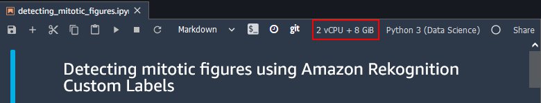
Some of the following steps require more RAM than what is available in a standard ml.t3.medium notebook. Make sure that you have selected an ml.m5.large notebook. You should see a 2 vCPU + 8 GiB indication on the upper right corner of the page.

The code for this section is available as a Jupyter notebook file.

After onboarding to Studio, follow these instructions to grant Studio the necessary permissions to call Amazon Rekognition on your behalf.

Dependencies

To begin with, we need to complete the following steps:

  1. Update Linux packages and install the required dependencies, such as OpenSlide:
    !apt update > /dev/null && apt dist-upgrade -y > /dev/null
    !apt install -y build-essential openslide-tools python-openslide libgl1-mesa-glx > /dev/null

  2. Install the fastai and SlideRunner libraries using pip:
    !pip install SlideRunner SlideRunner_dataAccess fastai==1.0.61 > /dev/null

  3. Download the dataset (we provide a script to do this automatically):
    from dataset import download_dataset
    download_dataset()

Process the dataset

We will begin by importing some of the packages that we use throughout the data preparation stage. Then, we download and load the annotation database for this dataset. This database contains the positions in the whole slide images of the mitotic figures (the features we want to classify). See the following code:

%reload_ext autoreload
%autoreload 2
import os
from typing import List
import urllib
import numpy as np
from SlideRunner.dataAccess.database import Database
from pathlib import Path

DATABASE_URL = 'https://github.com/DeepPathology/MITOS_WSI_CMC/raw/master/databases/MITOS_WSI_CMC_MEL.sqlite'
DATABASE_FILENAME = 'MITOS_WSI_CMC_MEL.sqlite'

Path("./databases").mkdir(parents=True, exist_ok=True)
local_filename, headers = urllib.request.urlretrieve(
    DATABASE_URL,
    filename=os.path.join('databases', DATABASE_FILENAME),
)

Because we’re using SageMaker, we create a new SageMaker session object to ease tasks such as uploading our dataset to an Amazon Simple Storage Service (Amazon S3) bucket. We also use the S3 bucket that SageMaker creates by default to upload our processed image files.

The slidelist_test array contains the IDs of the slides that we use as part of the test dataset to evaluate the performance of the trained model. See the following code:

import sagemaker
sm_session = sagemaker.Session()

size=512
bucket_name = sm_session.default_bucket()

database = Database()
database.open(os.path.join('databases', DATABASE_FILENAME))

slidelist_test = ['14','18','3','22','10','15','21']

The next step is to obtain a set of areas of training and test slides, along with the labels in them, from which we can take smaller areas to use to train our model. The code for get_slides is in the sampling.py file in GitHub.

from sampling import get_slides

image_size = 512

lbl_bbox, training_slides, test_slides, files = get_slides(database, slidelist_test, negative_class=1, size=image_size)

We want to randomly sample from the training and test slides. We use the lists of training and test slides and randomly select n_training_images times a file for training, and n_test_images times a file for test:

n_training_images = 500
n_test_images = int(0.2 * n_training_images)

training_files = list([
    (y, files[y]) for y in np.random.choice(
        [x for x in training_slides], n_training_images)
])
test_files = list([
    (y, files[y]) for y in np.random.choice(
        [x for x in test_slides], n_test_images)
])

Next, we create a directory for training images and one for test images:

Path("rek_slides/training").mkdir(parents=True, exist_ok=True)
Path("rek_slides/test").mkdir(parents=True, exist_ok=True)

Before we produce the smaller images needed to train the model, we need some helper code that produces the metadata needed to describe the training and test data. The following code makes sure that a given bounding box surrounding the features of interest (mitotic figures) are well within the zone we’re cutting, and produces a line of JSON that describes the image and the features in it in Amazon SageMaker Ground Truth format, which is the format Amazon Rekognition Custom Labels requires. For more information about this manifest file for object detection, see Object localization in manifest files.

def check_bbox(x_start: int, y_start: int, bbox) -> bool:
    return (bbox._left > x_start and
            bbox._right < x_start + image_size and
            bbox._top > y_start and
            bbox._bottom < y_start + image_size)
            

def get_annotation_json_line(filename, channel, annotations, labels):
    
    objects = list([{'confidence' : 1} for i in range(0, len(annotations))])
    
    return json.dumps({
        'source-ref': f's3://{bucket_name}/data/{channel}/{filename}',
        'bounding-box': {
            'image_size': [{
                'width': size,
                'height': size,
                'depth': 3
            }],
            'annotations': annotations,
        },
        'bounding-box-metadata': {
            'objects': objects,
            'class-map': dict({ x: str(x) for x in labels }),
            'type': 'groundtruth/object-detection',
            'human-annotated': 'yes',
            'creation-date': datetime.datetime.now().isoformat(),
            'job-name': 'rek-pathology',
        }
    })


def generate_annotations(x_start: int, y_start: int, bboxes, labels, filename: str, channel: str):
    annotations = []
    
    for bbox in bboxes:
        if check_bbox(x_start, y_start, bbox):
            # Get coordinates relative to this slide.
            x0 = bbox.left - x_start
            y0 = bbox.top - y_start
            
            annotation = {
                'class_id': 1,
                'top': y0,
                'left': x0,
                'width': bbox.right - bbox.left,
                'height': bbox.bottom - bbox.top
            }
            
            annotations.append(annotation)
    
    return get_annotation_json_line(filename, channel, annotations, labels)

With the generate_annotations function in place, we can write the code to produce the training and test images:

import datetime
import json
import random

from fastai import *
from fastai.vision import *
from tqdm.notebook import tqdm


# Margin size, in pixels, for training images. This is the space we leave on
# each side for the bounding box(es) to be well into the image.
margin_size = 64

training_annotations = []
test_annotations = []


def check_bbox(x_start: int, y_start: int, bbox) -> bool:
    return (bbox._left > x_start and
            bbox._right < x_start + image_size and
            bbox._top > y_start and
            bbox._bottom < y_start + image_size)


def generate_images(file_list) -> None:
    for f_idx in tqdm(range(0, len(file_list)), desc='Writing training images...'):
        slide_idx, f = file_list[f_idx]
        bboxes = lbl_bbox[slide_idx][0]
        labels = lbl_bbox[slide_idx][1]

        # Calculate the minimum and maximum horizontal and vertical positions
        # that bounding boxes should have within the image.
        x_min = min(map(lambda x: x.left, bboxes)) - margin_size
        y_min = min(map(lambda x: x.top, bboxes)) - margin_size
        x_max = max(map(lambda x: x.right, bboxes)) + margin_size
        y_max = max(map(lambda x: x.bottom, bboxes)) + margin_size

        result = False
        while not result:
            x_start = random.randint(x_min, x_max - image_size)
            y_start = random.randint(y_min, y_max - image_size)

            for bbox in bboxes:
                if check_bbox(x_start, y_start, bbox):
                    result = True
                    break

        filename = f'slide_{f_idx}.png'
        channel = 'test' if slide_idx in test_slides else 'training'
        annotation = generate_annotations(x_start, y_start, bboxes, labels, filename, channel)

        if channel == 'training':
            training_annotations.append(annotation)
        else:
            test_annotations.append(annotation)

        img = Image(pil2tensor(f.get_patch(x_start, y_start) / 255., np.float32))
        img.save(f'rek_slides/{channel}/{filename}')

generate_images(training_files)
generate_images(test_files)

The last step towards having all of the required data is to write a manifest.json file for each of the datasets:

with open('rek_slides/training/manifest.json', 'w') as mf:
    mf.write("n".join(training_annotations))

with open('rek_slides/test/manifest.json', 'w') as mf:
    mf.write("n".join(test_annotations))

Transfer the files to S3

We use the upload_data method that the SageMaker session object exposes to upload the images and manifest files to the default SageMaker S3 bucket:

import sagemaker


sm_session = sagemaker.Session()
data_location = sm_session.upload_data(
    './rek_slides',
    bucket=bucket_name,
)

Train an Amazon Rekognition Custom Labels model

With the data already in Amazon S3, we can get to training a custom model. We use the Boto3 library to create an Amazon Rekognition client and create a project:

import boto3

project_name = 'rek-mitotic-figures-workshop'

rek = boto3.client('rekognition')
response = rek.create_project(ProjectName=project_name)

# If you have already created the project, use the describe_projects call to
# retrieve the project ARN.
# response = rek.describe_projects()['ProjectDescriptions'][0]

project_arn = response['ProjectArn']

With the project ready to use, now you need a project version that points to the training and test datasets in Amazon S3. Each version ideally points to different datasets (or different versions of it). This enables us to have different versions of a model, compare their performance, and switch between them as needed. See the following code:

version_name = '1'

output_config = {
    'S3Bucket': bucket_name,
    'S3KeyPrefix': 'output',
}

training_dataset = {
    'Assets': [
        {
            'GroundTruthManifest': {
                'S3Object': {
                    'Bucket': bucket_name,
                    'Name': 'data/training/manifest.json'
                }
            },
        },
    ]
}

testing_dataset = {
    'Assets': [
        {
            'GroundTruthManifest': {
                'S3Object': {
                    'Bucket': bucket_name,
                    'Name': 'data/test/manifest.json'
                }
            },
        },
    ]
}


def describe_project_versions():
    describe_response = rek.describe_project_versions(
        ProjectArn=project_arn,
        VersionNames=[version_name],
    )

    for model in describe_response['ProjectVersionDescriptions']:
        print(f"Status: {model['Status']}")
        print(f"Message: {model['StatusMessage']}")
    
    return describe_response
    
    
response = rek.create_project_version(
    VersionName=version_name,
    ProjectArn=project_arn,
    OutputConfig=output_config,
    TrainingData=training_dataset,
    TestingData=testing_dataset,
)

waiter = rek.get_waiter('project_version_training_completed')
waiter.wait(
    ProjectArn=project_arn,
    VersionNames=[version_name],
)

describe_response = describe_project_versions()

After we create the project version, Amazon Rekognition automatically starts the training process. The training time depends on several features, such as the size of the images and the number of them, the number of classes, and so on. In this case, for 500 images, the training takes about 90 minutes to finish.

Test the model

After training, every model in Amazon Rekognition Custom Labels is in the STOPPED state. To use it for inference, you need to start it. We get the project version ARN from the project version description and pass it over to the start_project_version. Notice the MinInferenceUnits parameter — we start with one inference unit. The actual maximum number of transactions per second (TPS) that this inference unit supports depends on the complexity of your model. To learn more about TPS, refer to this blog post.

model_arn = describe_response['ProjectVersionDescriptions'][0]['ProjectVersionArn']

response = rek.start_project_version(
    ProjectVersionArn=model_arn,
    MinInferenceUnits=1,
)
waiter = rek.get_waiter('project_version_running')
waiter.wait(
    ProjectArn=project_arn,
    VersionNames=[version_name],
)

When your project version is listed as RUNNING, you can start sending images to Amazon Rekognition for inference.

We use one of the files in the test dataset to test the newly started model. You can use any suitable PNG or JPEG file instead.

from matplotlib import pyplot as plt
from PIL import Image, ImageDraw


# We'll use one of our test images to try out our model.
with open('./rek_slides/test/slide_0.png', 'rb') as image_file:
    image_bytes=image_file.read()


# Send the image data to the model.
response = rek.detect_custom_labels(
    ProjectVersionArn=model_arn,
    Image={
        'Bytes': image_bytes
    }
)

img = Image.open(io.BytesIO(image_bytes))
draw = ImageDraw.Draw(img)

for custom_label in response['CustomLabels']:
    geometry = custom_label['Geometry']['BoundingBox']
    w = geometry['Width'] * img.width
    h = geometry['Height'] * img.height
    l = geometry['Left'] * img.width
    t = geometry['Top'] * img.height
    draw.rectangle([l, t, l + w, t + h], outline=(0, 0, 255, 255), width=5)

plt.imshow(np.asarray(img))

Streamlit application

To demonstrate the integration with Amazon Rekognition, we use a very simple Python application. We use the Streamlit library to build a spartan user interface, where we prompt the user to upload an image file.

We use the Boto3 library and the detect_custom_labels method, together with the project version ARN, to invoke the inference endpoint. The response is a JSON document that contains the positions and classes of the different objects detected in the image. In our case, these are the mitotic figures that the algorithm has found in the image we sent to the endpoint. See the following code:

import os

import boto3
import io
import streamlit as st
from PIL import Image, ImageDraw


rek_client = boto3.client('rekognition')


uploaded_file = st.file_uploader('Image file')
if uploaded_file is not None:
    image_bytes = uploaded_file.read()
    result = rek_client.detect_custom_labels(
        ProjectVersionArn='<YOUR_PROJECT_ARN_HERE>',
        Image={
            'Bytes': image_bytes
        }
    )
    img = Image.open(io.BytesIO(image_bytes))
    draw = ImageDraw.Draw(img)

    st.write(result['CustomLabels'])
    for custom_label in result['CustomLabels']:
        st.write(f"Label {custom_label['Name']}, confidence {custom_label['Confidence']}")
        geometry = custom_label['Geometry']['BoundingBox']
        w = geometry['Width'] * img.width
        h = geometry['Height'] * img.height
        l = geometry['Left'] * img.width
        t = geometry['Top'] * img.height
        st.write(f"Left, top = ({l}, {t}), width, height = ({w}, {h})")
        draw.rectangle([l, t, l + w, t + h], outline=(0, 0, 255, 255), width=5)

    st_img = st.image(img)

Deploy the application to AWS

To deploy the application, we use an AWS CDK script. The whole project can be found on GitHub . Let’s look at the different resources deployed by the script.

Create an Amazon ECR repository

As the first step towards setting up our deployment, we create an Amazon ECR repository, where we can store our application container images:

aws ecr create-repository --repository-name rek-wsi

Create and store your GitHub token in AWS Secrets Manager

CodePipeline needs a GitHub Personal Access Token to monitor your GitHub repository for changes and pull code. To create the token, follow the instructions in the GitHub documentation. The token requires the following GitHub scopes:

  • The repo scope, which is used for full control to read and pull artifacts from public and private repositories into a pipeline.
  • The admin:repo_hook scope, which is used for full control of repository hooks.

After creating the token, store it in a new secret in AWS Secrets Manager as follows:

aws secretsmanager create-secret --name rek-wsi/github --secret-string "{"oauthToken":"YOUR-TOKEN-VALUE-HERE"}"

Write configuration parameters to AWS Systems Manager Parameter Store

The AWS CDK script reads some configuration parameters from AWS Systems Manager Parameter Store, such as the name and owner of the GitHub repository, and target account and Region. Before launching the AWS CDK script, you need to create these parameters in your own account.

You can do that by using the AWS CLI. Simply invoke the put-parameter command with a name, a value, and the type of the parameter:

aws ssm put-parameter --name <PARAMETER-NAME> --value <PARAMETER-VALUE> --type <PARAMETER_TYPE>

The following is a list of all parameters required by the AWS CDK script. All of them are of type String:

  • /rek_wsi/prod/accountId — The ID of the account where we deploy the application.
  • /rek_wsi/prod/ecr_repo_name — The name of the Amazon ECR repository where the container images are stored.
  • /rek_wsi/prod/github/branch — The branch in the GitHub repository from which CodePipeline needs to pull the code.
  • /rek_wsi/prod/github/owner — The owner of the GitHub repository.
  • /rek_wsi/prod/github/repo — The name of the GitHub repository where our code is stored.
  • /rek_wsi/prod/github/token — The name or ARN of the secret in Secrets Manager that contains your GitHub authentication token. This is necessary for CodePipeline to be able to communicate with GitHub.
  • /rek_wsi/prod/region — The region where we will deploy the application.

Notice the prod segment in all parameter names. Although we do not need this level of detail for such a simple example, it will enable to reuse this approach with other projects where different environments may be necessary.

Resources created by the AWS CDK script

We need our application, running in a Fargate task, to have permissions to invoke Amazon Rekognition. So we first create an AWS Identity and Access Management (IAM) Task Role with the RekognitionReadOnlyPolicy policy attached to it. Notice that the assumed_by parameter in the following code takes the ecs-tasks.amazonaws.com service principal. This is because we’re using Amazon ECS as the orchestrator, so we need Amazon ECS to assume the role and pass the credentials to the Fargate task.

streamlit_task_role = iam.Role(
    self, 'StreamlitTaskRole',
    assumed_by=iam.ServicePrincipal('ecs-tasks.amazonaws.com'),
    description='ECS Task Role assumed by the Streamlit task deployed to ECS+Fargate',
    managed_policies=[
        iam.ManagedPolicy.from_managed_policy_arn(
            self, 'RekognitionReadOnlyPolicy',
            managed_policy_arn='arn:aws:iam::aws:policy/AmazonRekognitionReadOnlyAccess'
        ),
    ],
)

Once built, our application container image sits in a private Amazon ECR repository. We need an object that describes it that we can pass when creating the Fargate service:

ecs_container_image = ecs.ContainerImage.from_ecr_repository(
    repository=ecr.Repository.from_repository_name(self, 'ECRRepo', 'rek-wsi'),
    tag='latest'
)

We create a new VPC and cluster for this application. You can modify this part to use your own VPC by using the from_lookup method of the Vpc class:

vpc = ec2.Vpc(self, 'RekWSI', max_azs=3)
cluster = ecs.Cluster(self, 'RekWSICluster', vpc=vpc)

Now that we have a VPC and cluster to deploy to, we create the Fargate service. We use 0.25 vCPU and 512 MB RAM for this task, and we place a public Application Load Balancer (ALB) in front of it. Once deployed, we use the ALB CNAME to access the application. See the following code:

fargate_service = ecs_patterns.ApplicationLoadBalancedFargateService(
    self, 'RekWSIECSApp',
    cluster=cluster,
    cpu=256,
    memory_limit_mib=512,
    desired_count=1,
    task_image_options=ecs_patterns.ApplicationLoadBalancedTaskImageOptions(
        image=ecs_container_image,
        container_port=8501,
        task_role=streamlit_task_role,
    ),
    public_load_balancer=True,
)

To automatically build and deploy a new container image every time we push code to our main branch, we create a simple pipeline consisting of a GitHub source action and a build step. Here is where we use the secrets we stored in AWS Secrets Manager and AWS Systems Manager Parameter Store in the previous steps.

pipeline = codepipeline.Pipeline(self, 'RekWSIPipeline')

# Create an artifact that points at the code pulled from GitHub.
source_output = codepipeline.Artifact()

# Create a source stage that pulls the code from GitHub. The repo parameters are
# stored in SSM, and the OAuth token in Secrets Manager.
source_action = codepipeline_actions.GitHubSourceAction(
    action_name='GitHub',
    output=source_output,
    oauth_token=SecretValue.secrets_manager(
        ssm.StringParameter.value_from_lookup(self, '/rek_wsi/prod/github/token'),
        json_field='oauthToken'),
    trigger=codepipeline_actions.GitHubTrigger.WEBHOOK,
    owner=ssm.StringParameter.value_from_lookup(self, '/rek_wsi/prod/github/owner'),
    repo=ssm.StringParameter.value_from_lookup(self, '/rek_wsi/prod/github/repo'),
    branch=ssm.StringParameter.value_from_lookup(self, '/rek_wsi/prod/github/branch'),
)

# Add the source stage to the pipeline.
pipeline.add_stage(
    stage_name='GitHub',
    actions=[source_action]
)

CodeBuild needs permissions to push container images to Amazon ECR. To grant these permissions, we add the AmazonEC2ContainerRegistryFullAccess policy to a bespoke IAM role that the CodeBuild service principal can assume:

# Create an IAM role that grants CodeBuild access to Amazon ECR to push containers.
build_role = iam.Role(
    self,
    'RekWsiCodeBuildAccessRole',
    assumed_by=iam.ServicePrincipal('codebuild.amazonaws.com'),
)

# Permissions are granted through an AWS managed policy, AmazonEC2ContainerRegistryFullAccess.
managed_ecr_policy = iam.ManagedPolicy.from_managed_policy_arn(
    self, 'cb_ecr_policy',
    managed_policy_arn='arn:aws:iam::aws:policy/AmazonEC2ContainerRegistryFullAccess',
)
build_role.add_managed_policy(policy=managed_ecr_policy)

The CodeBuild project logs into the private Amazon ECR repository, builds the Docker image with the Streamlit application, and pushes the image into the repository together with an appspec.yaml and an imagedefinitions.json file.

The appspec.yaml file describes the task (port, Fargate platform version, and so on), while the imagedefinitions.json file maps the names of the container images to their corresponding Amazon ECR URI. See the following code:

container_name = fargate_service.task_definition.default_container.container_name
build_project = codebuild.PipelineProject(
    self,
    'RekWSIProject',
    build_spec=codebuild.BuildSpec.from_object({
        'version': '0.2',
        'phases': {
            'pre_build': {
                'commands': [
                    'env',
                    'COMMIT_HASH=$(echo $CODEBUILD_RESOLVED_SOURCE_VERSION | cut -c 1-7)',
                    'export TAG=${COMMIT_HASH:=latest}',
                    'aws ecr get-login-password --region $AWS_DEFAULT_REGION | '
                    'docker login --username AWS '
                    '--password-stdin $AWS_ACCOUNT_ID.dkr.ecr.$AWS_DEFAULT_REGION.amazonaws.com',
                ]
            },
            'build': {
                'commands': [
                    # Build the Docker image
                    'cd streamlit_app && docker build -t $IMAGE_REPO_NAME:$IMAGE_TAG .',
                    # Tag the image
                    'docker tag $IMAGE_REPO_NAME:$IMAGE_TAG '
                    '$AWS_ACCOUNT_ID.dkr.ecr.$AWS_DEFAULT_REGION.amazonaws.com/$IMAGE_REPO_NAME:$IMAGE_TAG',
                ]
            },
            'post_build': {
                'commands': [
                    # Push the container into ECR.
                    'docker push '
                    '$AWS_ACCOUNT_ID.dkr.ecr.$AWS_DEFAULT_REGION.amazonaws.com/$IMAGE_REPO_NAME:$IMAGE_TAG',
                    # Generate imagedefinitions.json
                    'cd ..',
                    "printf '[{"name":"%s","imageUri":"%s"}]' "
                    f"{container_name} "
                    "$AWS_ACCOUNT_ID.dkr.ecr.$AWS_DEFAULT_REGION.amazonaws.com/$IMAGE_REPO_NAME:$IMAGE_TAG "
                    "> imagedefinitions.json",
                    'ls -l',
                    'pwd',
                    'sed -i s"|REGION_NAME|$AWS_DEFAULT_REGION|g" appspec.yaml',
                    'sed -i s"|ACCOUNT_ID|$AWS_ACCOUNT_ID|g" appspec.yaml',
                    'sed -i s"|TASK_NAME|$IMAGE_REPO_NAME|g" appspec.yaml',
                    f'sed -i s"|CONTAINER_NAME|{container_name}|g" appspec.yaml',
                ]
            }
        },
        'artifacts': {
            'files': [
                'imagedefinitions.json',
                'appspec.yaml',
            ],
        },
    }),
    environment=codebuild.BuildEnvironment(
        build_image=codebuild.LinuxBuildImage.STANDARD_5_0,
        privileged=True,
    ),
    environment_variables={
        'AWS_ACCOUNT_ID':
            codebuild.BuildEnvironmentVariable(value=self.account),
        'IMAGE_REPO_NAME':
            codebuild.BuildEnvironmentVariable(
                value=ssm.StringParameter.value_from_lookup(self, '/rek_wsi/prod/ecr_repo_name')),
        'IMAGE_TAG':
            codebuild.BuildEnvironmentVariable(value='latest'),
    },
    role=build_role,
)

Finally, we put the different pipeline stages together. The last action is the EcsDeployAction, which takes the container image built in the previous stage and does a rolling update of the tasks in our ECS cluster:

# Create an artifact to store the build output.
build_output = codepipeline.Artifact()
# Create a build action that ties the build project, the source artifact from the
# previous stage, and the output artifact together.
build_action = codepipeline_actions.CodeBuildAction(
    action_name='Build',
    project=build_project,
    input=source_output,
    outputs=[build_output],
)
# Add the build stage to the pipeline.
pipeline.add_stage(
    stage_name='Build',
    actions=[build_action]
)
deploy_action = codepipeline_actions.EcsDeployAction(
    action_name='Deploy',
    service=fargate_service.service,
    # image_file=build_output
    input=build_output,
)
pipeline.add_stage(
    stage_name='Deploy',
    actions=[deploy_action],
)

Cleanup

To avoid incurring future costs, clean up the resources you created as part of this solution.

Amazon Rekognition Custom Labels model

Before you shut down your Studio notebook, make sure you stop the Amazon Rekognition Custom Labels model. If you don’t, it continues to incur costs.

rek.stop_project_version(
    ProjectVersionArn=model_arn,
)

Alternatively, you can use the Amazon Rekognition console to stop the service:

  1. On the Amazon Rekognition console, choose Use Custom Labels in the navigation pane.
  2. Choose Projects in the navigation pane.
  3. Choose version 1 of the rek-mitotic-figures-workshop project.
  4. On the Use Model tab, choose Stop.

Streamlit application

To destroy all resources associated to the Streamlit application, run the following code from the AWS CDK application directory:

cdk destroy RekWsiStack

AWS Secrets Manager

To delete the GitHub token, follow the instructions in the documentation.

Conclusion

In this post, we walked through the necessary steps to train a Amazon Rekognition Custom Labels model for a digital pathology application using real-world data. We then learned how to use the model from a simple application deployed from a CI/CD pipeline to Fargate.

Amazon Rekognition Custom Labels enables you to build ML-enabled healthcare applications that you can easily build and deploy using services like Fargate, CodeBuild, and CodePipeline.

Can you think of any applications to help researchers, doctors, or their patients to make their lives easier? If so, use the code in this walkthrough to build your next application. And if you have any questions, please share them in the comments section.

Acknowledgments

We would like to thank Prof. Dr. Marc Aubreville for kindly giving us permission to use the MITOS_WSI_CMC dataset for this blog post. The dataset can be found on GitHub.

References

[1] Aubreville, M., Bertram, C.A., Donovan, T.A. et al. A completely annotated whole slide image dataset of canine breast cancer to aid human breast cancer research. Sci Data 7, 417 (2020). https://doi.org/10.1038/s41597-020-00756-z

[2] Khened, M., Kori, A., Rajkumar, H. et al. A generalized deep learning framework for whole-slide image segmentation and analysis. Sci Rep 11, 11579 (2021). https://doi.org/10.1038/s41598-021-90444-8

[3] PNAS March 27, 2018 115 (13) E2970-E2979; first published March 12, 2018; https://doi.org/10.1073/pnas.1717139115


About the Author

Pablo Nuñez Pölcher, MSc, is a Senior Solutions Architect working for the Public Sector team with Amazon Web Services. Pablo focuses on helping healthcare public sector customers build new, innovative products on AWS in accordance with best practices. He received his M.Sc. in Biological Sciences from Universidad de Buenos Aires. In his spare time, he enjoys cycling and tinkering with ML-enabled embedded devices.

Razvan Ionasec, PhD, MBA, is the technical leader for healthcare at Amazon Web Services in Europe, Middle East, and Africa. His work focuses on helping healthcare customers solve business problems by leveraging technology. Previously, Razvan was the global head of artificial intelligence (AI) products at Siemens Healthineers in charge of AI-Rad Companion, the family of AI-powered and cloud-based digital health solutions for imaging. He holds 30+ patents in AI/ML for medical imaging and has published 70+ international peer-reviewed technical and clinical publications on computer vision, computational modeling, and medical image analysis. Razvan received his PhD in Computer Science from the Technical University Munich and MBA from University of Cambridge, Judge Business School.

Read More

Distributed fine-tuning of a BERT Large model for a Question-Answering Task using Hugging Face Transformers on Amazon SageMaker

From training new models to deploying them in production, Amazon SageMaker offers the most complete set of tools for startups and enterprises to harness the power of machine learning (ML) and Deep Learning.

With its Transformers open-source library and ML platform, Hugging Face makes transfer learning and the latest ML models accessible to the global AI community, reducing the time needed for data scientists and ML engineers in companies around the world to take advantage of every new scientific advancement.

Applying Transformers to new NLP tasks or domains requires fine-tuning of large language models, a technique leveraging the accumulated knowledge of pre-trained models to adapt them to a new task or specific type of documents in an additional, efficient training process.

Fine-tuning the model to produce accurate predictions for the business problem at hand requires the training of large Transformers models, for example, BERT, BART, RoBERTa, T5, which can be challenging to perform in a scalable way.

Hugging Face has been working closely with SageMaker to deliver ready-to-use Deep Learning Containers (DLCs) that make training and deploying the latest Transformers models easier and faster than ever. Because features such as SageMaker Data Parallel (SMDP), SageMaker Model Parallel (SMMP), S3 pipe mode, are integrated into the container, using these drastically reduces the time for companies to create Transformers-based ML solutions such as question-answering, generating text and images, optimizing search results, and improves customer support automation, conversational interfaces, semantic search, document analyses, and many more applications.

In this post, we focus on the deep integration of SageMaker distributed libraries with Hugging Face, which enables data scientists to accelerate training and fine-tuning of Transformers models from days to hours, all in SageMaker.

Overview of distributed training

ML practitioners and data scientists face two scaling challenges when training models: scaling model size (number of parameters and layers) and scaling training data. Scaling either the model size or training data can result in better accuracy, but there can be cases in deep learning where the amount of memory on the accelerator (CPU or GPU) limits the combination of the size of the training data and the size of the model. For example, when training a large language model, the batch size is often limited to a small number of samples, which can result in a less accurate model.

Distributed training can split up the workload to train the model among multiple processors, called workers. These workers operate in parallel to speed up model training.

Based on what we want to scale (model or data) there are two approaches to distributed training: data parallel and model parallel.

Data parallel is the most common approach to distributed training. Data parallelism entails creating a copy of the model architecture and weights on different accelerators. Then, rather than passing in the entire training set to a single accelerator, we can partition the training set across the different accelerators, and get through the training set faster. Although this adds the step of the accelerators needing to communicate their gradient information back to a parameter server, this time is more than offset by the speed boost of iterating over a fraction of the entire dataset per accelerator. Because of this, data parallelism can significantly help reduce training times. For example, training a single model without parallelization takes 4 hours. Using distributed training can reduce that to 24 minutes. SageMaker distributed training also implements cutting-edge techniques in gradient updates.

A model parallel approach is used with large models too large to fit on one accelerator (GPU). This approach implements a parallelization strategy where the model architecture is divided into shards and placed onto different accelerators. The configuration of each of these shards is neural network architecture dependent, and typically includes several layers. The communication between the accelerators occurs each time the training data passes from one of the shards to the next.

To summarize, you should use distributed training data parallelism for time-intensive tasks due to large datasets or when you want to accelerate your training experiments. You should use model parallelism when your model can’t fit onto one accelerator.

Prerequisites

To perform distributed training of Hugging Face Transformers models in SageMaker, you need to complete the following prerequisites:

Implement distributed training

The Hugging Face Transformers library provides a Trainer API that is optimized to train or fine-tune the models the library provides. You can also use it on your own models if they work the same way as Transformers models; see Trainer for more details. This API is used in our example scripts, which show how to preprocess the data for various NLP tasks, which you can take as models to write a script solving your own custom problem. The promise of the Trainer API is that this script works out of the box on any distributed setup, including SageMaker.

The Trainer API takes everything needed for the training. This includes your datasets, your model (or a function that returns your model), a compute_metrics function that returns the metrics you want to track from the arrays of predications and labels, your optimizer and learning rate scheduler (good defaults are provided), as well as all the hyperparameters you can tune for your training grouped in a data class called TrainingArguments. With all of that, it exposes three methods—train, evaluate, and predict—to train your model, get the metric results on any dataset, or get the predictions on any dataset. To learn more about the Trainer object, refer to Fine-tuning a model with the Trainer API and the video The Trainer API, which walks you through a simple example.

Behind the scenes, the Trainer API starts by analyzing the environment in which you are launching your script when you create the TrainingArguments. For instance, if you launched your training with SageMaker, it looks at the SM_FRAMEWORK_PARAMS variable in the environment to detect if you enabled SageMaker data parallelism or model parallelism. Then it gets the relevant variables (such as the rank of the process or the world size) from the environment before performing the necessary initialization steps (such as smdistributed.dataparallel.torch.distributed.init_process_group()).

The Trainer contains the whole training loop, so it can adjust the necessary steps to make sure the smdistributed.dataparallel backend is used when necessary without you having to change a line of code in your script. It can still run (albeit much slower) on your local machine for debugging. It handles sharding your dataset such that each process sees different samples automatically, with a reshuffle at each epoch, synchronizing your gradients before the optimization step, mixed precision training if you activated it, gradient accumulation if you can’t fit a big batch size on your GPUs, and many more optimizations.

If you activated model parallelism, it makes sure the processes that have to see the same data (if their dp_rank is the same) get the same batches, and that processes with different dp_rank don’t see the same samples, again with a reshuffle at each epoch. It makes sure the state dictionaries of the model or optimizers are properly synchronized when checkpointing, and again handles all the optimizations such as mixed precision and gradient accumulation.

When using the evaluate and predict methods, the Trainer performs a distributed evaluation, to take advantage of all your GPUs. It properly handles splitting your data for each process (process of the same dp_rank if model parallelism is activated) and makes sure that the predictions are properly gathered in the same order as the dataset you’re using before they are sent to the compute_metrics function or just returned. Using the Trainer API is not mandatory. Users can still use Keras or PyTorch within Hugging Face. However, the Trainer API can provide a helpful abstraction layer.

Train a model using SageMaker Hugging Face Estimators

An Estimator is a high-level interface for SageMaker training and handles end-to-end SageMaker training and deployment tasks. The training of your script is invoked when you call fit on a HuggingFace Estimator. In the Estimator, you define which fine-tuning script to use as entry_point, which instance_type to use, and which hyperparameters are passed in. For more information about HuggingFace parameters, see Hugging Face Estimator.

Distributed training: Data parallel

In this example, we use the new Hugging Face DLCs and SageMaker SDK to train a distributed Seq2Seq-transformer model on the question and answering task using the Transformers and datasets libraries. The bert-large-uncased-whole-word-masking model is fine-tuned on the squad dataset.

The following code samples show you steps of creating a HuggingFace estimator for distributed training with data parallelism.

  1. Choose a Hugging Face Transformers script:
    # git configuration to download our fine-tuning script
    git_config = {'repo': 'https://github.com/huggingface/transformers.git','branch': 'v4.6.1'}

When you create a HuggingFace Estimator, you can specify a training script that is stored in a GitHub repository as the entry point for the Estimator, so you don’t have to download the scripts locally. You can use git_config to run the Hugging Face Transformers examples scripts and right ‘branch’ if your transformers_version needs to be configured. For example, if you use transformers_version 4.6.1, you have to use ‘branch':'v4.6.1‘.

  1. Configure training hyperparameters that are passed into the training job:
    # hyperparameters, which are passed into the training job
    hyperparameters={
        'model_name_or_path': 'bert-large-uncased-whole-word-masking',
        'dataset_name':'squad',
        'do_train': True,
        'do_eval': True,
        'fp16': True,
        'per_device_train_batch_size': 4,
        'per_device_eval_batch_size': 4,
        'num_train_epochs': 2,
        'max_seq_length': 384,
        'max_steps': 100,
        'pad_to_max_length': True,
        'doc_stride': 128,
        'output_dir': '/opt/ml/model'
    }

As a hyperparameter, we can define any Seq2SeqTrainingArguments and the ones defined in the training script.

  1. Define the distribution parameters in the HuggingFace Estimator:
    # configuration for running training on smdistributed Data Parallel
    distribution = {'smdistributed':{'dataparallel':{ 'enabled': True }}}

You can use the SageMaker data parallelism library out of the box for distributed training. We added the functionality of data parallelism directly into the Trainer. To enable data parallelism, you can simply add a single parameter to your HuggingFace Estimator to let your Trainer-based code use it automatically.

  1. Create a HuggingFace Estimator including parameters defined in previous steps and start training:
from sagemaker.huggingface import HuggingFace
# estimator
huggingface_estimator = HuggingFace(entry_point='run_qa.py',
                                    source_dir='./examples/pytorch/question-answering',
                                    git_config=git_config,
                                    instance_type= 'ml.p3.16xlarge',
                                    instance_count= 2,
                                    volume_size= 200,
                                    role= <SageMaker Role>, # IAM role,
                                    transformers_version='4.6',
                                    pytorch_version='1.7',
                                    py_version='py36',
                                    distribution= distribution,
                                    hyperparameters = hyperparameters)

# starting the train job 
huggingface_estimator.fit()

The Hugging Face Transformers repository contains several examples and scripts for fine-tuning models on tasks from language modeling to token classification. In our case, we use run_qa.py from the examples/pytorch/question-answering examples.

smdistributed.dataparallel supports model training on SageMaker with the following instance types only. For best performance, we recommend using an instance type that supports Elastic Fabric Adapter (EFA):

  • ml.p3.16xlarge
  • ml.p3dn.24xlarge (Recommended)
  • ml.p4d.24xlarge (Recommended)

To get the best performance and the most out of SMDataParallel, you should use at least two instances, but you can also use one for testing this example.

The following example notebook provides more detailed step-by-step guidance.

Distributed training: Model parallel

For distributed training with model parallelism, we use the Hugging Face Transformers and datasets library together with the SageMaker SDK for sequence classification on the General Language Understanding Evaluation (GLUE) benchmark on a multi-node, multi-GPU cluster using the SageMaker model parallelism library.

As with data parallelism, we first set the git configuration, training hyperparameters, and distribution parameters in the HuggingFace Estimator:

# git configuration to download our fine-tuning script
git_config = {'repo': 'https://github.com/huggingface/transformers.git','branch': 'v4.6.1'}

# hyperparameters, which are passed into the training job
hyperparameters={
    'model_name_or_path':'roberta-large',
    'task_name': 'mnli',
    'per_device_train_batch_size': 16,
    'per_device_eval_batch_size': 16,
    'do_train': True,
    'do_eval': True,
    'do_predict': True,
    'num_train_epochs': 2,
    'output_dir':'/opt/ml/model',
    'max_steps': 500,
}

# configuration for running training on smdistributed Model Parallel
mpi_options = {
    "enabled" : True,
    "processes_per_host" : 8,
}
smp_options = {
    "enabled":True,
    "parameters": {
        "microbatches": 4,
        "placement_strategy": "spread",
        "pipeline": "interleaved",
        "optimize": "speed",
        "partitions": 4,
        "ddp": True,
    }
}

distribution={
    "smdistributed": {"modelparallel": smp_options},
    "mpi": mpi_options
}

The model parallelism library internally uses MPI, so to use model parallelism, MPI must be enabled using the distribution parameter. “processes_per_host” in the preceding code specifies the number of processes MPI should launch on each host. We suggest these for development and testing. At production time, you can contact AWS Support if requesting extensive GPU capacity. For more information, see Run a SageMaker Distributed Model Parallel Training Job.

The following example notebook contains the complete code scripts.

Spot Instances

With the Hugging Face framework extension for the SageMaker Python SDK, we can also take advantage of fully managed Amazon Elastic Compute Cloud (Amazon EC2) Spot Instances and save up to 90% of our training cost.

Unless your training job will complete quickly, we recommend you use checkpointing with managed spot training, therefore you need to define checkpoint_s3_uri.

To use Spot Instances with the HuggingFace Estimator, we have to set the use_spot_instances parameter to True and define your max_wait and max_run time. For more information about the managed spot training lifecycle, see Managed Spot Training in Amazon SageMaker.

The following is a code snippet for setting up a spot training Estimator:

from sagemaker.huggingface import HuggingFace

# hyperparameters, which are passed into the training job
hyperparameters={'epochs': 1,
                 'train_batch_size': 32,
                 'model_name':'distilbert-base-uncased',
                 'output_dir':'/opt/ml/checkpoints'
                 }

# s3 uri where our checkpoints will be uploaded during training
job_name = "using-spot"
checkpoint_s3_uri = f's3://{sess.default_bucket()}/{job_name}/checkpoints'

huggingface_estimator = HuggingFace(entry_point='train.py',
                            source_dir='./scripts',
                            instance_type='ml.p3.2xlarge',
                            instance_count=1,
                            base_job_name=job_name,
                            checkpoint_s3_uri=checkpoint_s3_uri,
                            use_spot_instances=True,
                            max_wait=3600, # This should be equal to or greater than max_run in seconds'
                            max_run=1000, # expected max run in seconds
                            role=role,
                            transformers_version='4.6',
                            pytorch_version='1.7',
                            py_version='py36',
                            hyperparameters = hyperparameters)

The following notebook contains the complete code scripts.

Conclusion

In this post, we discussed distributed training of Hugging Face Transformers using SageMaker. We first reviewed the use cases for data parallelism vs. model parallelism. Data parallelism is typically more appropriate but not necessarily restricted to when training is bottlenecked by compute, whereas you can use model parallelism when a model can’t fit within the memory provided on a single accelerator. We then showed how to train with both methods.

In the data parallelism use case we discussed, training a model on a single p3.2xlarge instance (with a single GPU) takes 4 hours and costs roughly $15 at the time of this writing. With data parallelism, we can train the same model in 24 minutes at a cost of $28. Although the cost has doubled, this has reduced the training time by a factor of 10. For a situation in which you need to train many models within a short period of time, data parallelism can enable this at a relatively low cost increase. As for the model parallelism use case, it adds the ability to train models that could not have been previously trained at all due to hardware limitations. Both features enable new workflows for ML practitioners, and are readily accessible through the HuggingFace Estimator as a part of the SageMaker Python SDK. Deploying these models to hosted endpoints follows the same procedure as for other Estimators.

This integration enables other features that are part of the SageMaker ecosystem. For example, you can use Spot Instances by adding a simple flag to the Estimator for additional cost-optimization. As a next step, you can find and run the training demo and example notebook.


About the Authors

Archis Joglekar is an AI/ML Partner Solutions Architect in the Emerging Technologies team. He is interested in performant, scalable deep learning and scientific computing using the building blocks at AWS. His past experiences range from computational physics research to machine learning platform development in academia, national labs, and startups. His time away from the computer is spent playing soccer and with friends and family.

James Yi is a Sr. AI/ML Partner Solutions Architect in the Emerging Technologies team at Amazon Web Services. He is passionate about working with enterprise customers and partners to design, deploy and scale AI/ML applications to derive their business values. Outside of work, he enjoys playing soccer, traveling and spending time with his family.

Philipp Schmid is a Machine Learning Engineer and Tech Lead at Hugging Face, where he leads the collaboration with the Amazon SageMaker team. He is passionate about democratizing, optimizing, and productionizing cutting-edge NLP models and improving the ease of use for Deep Learning.

Sylvain Gugger is a Research Engineer at Hugging Face and one of the main maintainers of the Transformers library. He loves open source software and help the community use it.

Jeff Boudier builds products at Hugging Face, creator of Transformers, the leading open-source ML library. Previously Jeff was a co-founder of Stupeflix, acquired by GoPro, where he served as director of Product Management, Product Marketing, Business Development and Corporate Development.

Read More