Monthly Archives: June 2022

Many applications meant for industrial equipment maintenance, trade monitoring, fleet management, and route optimization are built using open-source Cassandra APIs and drivers to process data at high speeds and low latency. Managing Cassandra tables yourself can be time consuming and expensive. Amazon Keyspaces (for Apache Cassandra) lets you set up, secure, and scale Cassandra tables in the AWS Cloud without managing additional infrastructure.

In this post, we’ll walk you through AWS Services related to training machine learning (ML) models using Amazon Keyspaces at a high level, and provide step by step instructions for ingesting data from Amazon Keyspaces into Amazon SageMaker and training a model which can be used for a specific customer segmentation use case.

AWS has multiple services to help businesses implement ML processes in the cloud.

AWS ML Stack has three layers. In the middle layer is SageMaker, which provides developers, data scientists, and ML engineers with the ability to build, train, and deploy ML models at scale. It removes the complexity from each step of the ML workflow so that you can more easily deploy your ML use cases. This includes anything from predictive maintenance to computer vision to predict customer behaviors. Customers achieve up to 10 times improvement in data scientists’ productivity with SageMaker.

Apache Cassandra is a popular choice for read-heavy use cases with un-structured or semi-structured data. For example, a popular food delivery business estimates time of delivery, and a retail customer could persist frequently using product catalog information in the Apache Cassandra Database. Amazon Keyspaces is a scalable, highly available, and managed serverless Apache Cassandra–compatible database service. You don’t need to provision, patch, or manage servers, and you don’t need to install, maintain, or operate software. Tables can scale up and down automatically, and you only pay for the resources that you use. Amazon Keyspaces lets you you run your Cassandra workloads on AWS using the same Cassandra application code and developer tools that you use today.

SageMaker provides a suite of built-in algorithms to help data scientists and ML practitioners get started training and deploying ML models quickly. In this post, we’ll show you how a retail customer can use customer purchase history in the Keyspaces Database and target different customer segments for marketing campaigns.

K-means is an unsupervised learning algorithm. It attempts to find discrete groupings within data, where members of a group are as similar as possible to one another and as different as possible from members of other groups. You define the attributes that you want the algorithm to use to determine similarity. SageMaker uses a modified version of the web-scale k-means clustering algorithm. As compared with the original version of the algorithm, the version used by SageMaker is more accurate. However, like the original algorithm, it scales to massive datasets and delivers improvements in training time.

Solution overview

The instructions assume that you would be using SageMaker Studio to run the code. The associated code has been shared on AWS Sample GitHub. Following the instructions in the lab, you can do the following:

• Install necessary dependencies.
• Connect to Amazon Keyspaces, create a Table, and ingest sample data.
• Build a classification ML model using the data in Amazon Keyspaces.
• Explore model results.
• Clean up newly created resources.

Once complete, you’ll have integrated SageMaker with Amazon Keyspaces to train ML models as shown in the following image.

Now you can follow the step-by-step instructions in this post to ingest raw data stored in Amazon Keyspaces using SageMaker and the data thus retrieved for ML processing.

Prerequisites

First, Navigate to SageMaker.

Next, if this is the first time that you’re using SageMaker, select Get Started.

Next, select Setup up SageMaker Domain.

Next, create a new user profile with Name – sagemakeruser, and select Create New Role in the Default Execution Role sub section.

Next, in the screen that pops up, select any Amazon Simple Storage Service (Amazon S3) bucket, and select Create role.

This role will be used in the following steps to allow SageMaker to access Keyspaces Table using temporary credentials from the role. This eliminates the need to store a username and password in the notebook.

Next, retrieve the role associated with the sagemakeruser that was created in the previous step from the summary section.

Then, navigate to the AWS Console and look up AWS Identity and Access Management (IAM). Within IAM, navigate to Roles. Within Roles, search for the execution role identified in the previous step.

Next, select the role identified in the previous step and select Add Permissions. In the drop down that appears, select Create Inline Policy. SageMaker lets you provide a granular level of access that restricts what actions a user/application can perform based on business requirements.

Then, select the JSON tab and copy the policy from the Note section of Github page. This policy allows the SageMaker notebook to connect to Keyspaces and retrieve data for further processing.

Then, select Add permissions again and from the drop down, and select Attach Policy.

Lookup AmazonKeyspacesFullAccess policy, and select the checkbox next to the matching result, and select Attach Policies.

Verify that the permissions policies section includes AmazonS3FullAccess, AmazonSageMakerFullAccess, AmazonKeyspacesFullAccess, as well as the newly added inline policy.

Next, navigate to SageMaker Studio using the AWS Console and select the SageMaker Studio. Once there, select Launch App and select Studio.

Notebook walkthrough

The preferred way to connect to Keyspaces from SageMaker Notebook is by using AWS Signature Version 4 process (SigV4) based Temporary Credentials for authentication. In this scenario, we do NOT need to generate or store Keyspaces credentials and can use the credentials to authenticate with the SigV4 plugin. Temporary security credentials consist of an access key ID and a secret access key. However, they also include a security token that indicates when the credentials expire. In this post, we’ll create an IAM role and generate temporary security credentials.

First, we install a driver (cassandra-sigv4). This driver enables you to add authentication information to your API requests using the AWS Signature Version 4 Process (SigV4). Using the plugin, you can provide users and applications with short-term credentials to access Amazon Keyspaces (for Apache Cassandra) using IAM users and roles. Following this, you’ll import a required certificate along with additional package dependencies. In the end, you will allow the notebook to assume the role to talk to Keyspaces.

# Install missing packages and import dependencies
# Installing Cassandra SigV4
%pip install  cassandra-sigv4

# Get Security certificate
!curl https://certs.secureserver.net/repository/sf-class2-root.crt -O

# Import
from sagemaker import get_execution_role
from cassandra.cluster import Cluster
from ssl import SSLContext, PROTOCOL_TLSv1_2, CERT_REQUIRED
from cassandra_sigv4.auth import SigV4AuthProvider
import boto3

import pandas as pd
from pandas import DataFrame

import csv
from cassandra import ConsistencyLevel
from datetime import datetime
import time
from datetime import timedelta

import pandas as pd
import datetime as dt
import seaborn as sns
import matplotlib.pyplot as plt
from sklearn.cluster import KMeans
from sklearn.preprocessing import MinMaxScaler

# Getting credentials from the role
client = boto3.client("sts")

# Get notebook Role
role = get_execution_role()
role_info = {"RoleArn": role, "RoleSessionName": "session1"}
print(role_info)

credentials = client.assume_role(**role_info)

Next, connect to Amazon Keyspaces and read systems data from Keyspaces into Pandas DataFrame to validate the connection.

# Connect to Cassandra Database from SageMaker Notebook 
# using temporary credentials from the Role.
session = boto3.session.Session()

###
### You can also pass specific credentials to the session
###
#session = boto3.session.Session(
# aws_access_key_id=credentials["Credentials"]["AccessKeyId"],
# aws_secret_access_key=credentials["Credentials"]["SecretAccessKey"],
# aws_session_token=credentials["Credentials"]["SessionToken"],
#)

region_name = session.region_name

# Set Context
ssl_context = SSLContext(PROTOCOL_TLSv1_2)
ssl_context.load_verify_locations("sf-class2-root.crt")
ssl_context.verify_mode = CERT_REQUIRED

auth_provider = SigV4AuthProvider(session)
keyspaces_host = "cassandra." + region_name + ".amazonaws.com"

cluster = Cluster([keyspaces_host], ssl_context=ssl_context, auth_provider=auth_provider, port=9142)
session = cluster.connect()

# Read data from Keyspaces system table. 
# Keyspaces is serverless DB so you don't have to create Keyspaces DB ahead of time.
r = session.execute("select * from system_schema.keyspaces")

# Read Keyspaces row into Panda DataFrame
df = DataFrame(r)
print(df)

Next, prepare the data for training on the raw data set. In the python notebook associated with this post, use a retail data set downloaded from here, and process it. Our business objective given the data set is to cluster the customers using a specific metric call RFM. The RFM model is based on three quantitative factors:

• Recency: How recently a customer has made a purchase.
• Frequency: How often a customer makes a purchase.
• Monetary Value: How much money a customer spends on purchases.

RFM analysis numerically ranks a customer in each of these three categories, generally on a scale of 1 to 5 (the higher the number, the better the result). The “best” customer would receive a top score in every category. We’ll use pandas’s Quantile-based discretization function (qcut). It will help discretize values into equal-sized buckets based or based on sample quantiles.

# Prepare Data
r = session.execute("select * from " + keyspaces_schema + ".online_retail")

df = DataFrame(r)
df.head(100)

df.count()
df["description"].nunique()
df["totalprice"] = df["quantity"] * df["price"]
df.groupby("invoice").agg({"totalprice": "sum"}).head()

df.groupby("description").agg({"price": "max"}).sort_values("price", ascending=False).head()
df.sort_values("price", ascending=False).head()
df["country"].value_counts().head()
df.groupby("country").agg({"totalprice": "sum"}).sort_values("totalprice", ascending=False).head()

returned = df[df["invoice"].str.contains("C", na=False)]
returned.sort_values("quantity", ascending=True).head()

df.isnull().sum()
df.dropna(inplace=True)
df.isnull().sum()
df.dropna(inplace=True)
df.isnull().sum()
df.describe([0.05, 0.01, 0.25, 0.50, 0.75, 0.80, 0.90, 0.95, 0.99]).T
df.drop(df.loc[df["customer_id"] == ""].index, inplace=True)

# Recency Metric
import datetime as dt

today_date = dt.date(2011, 12, 9)
df["customer_id"] = df["customer_id"].astype(int)

# create get the most recent invoice for each customer
temp_df = df.groupby("customer_id").agg({"invoice_date": "max"})
temp_df["invoice_date"] = temp_df["invoice_date"].astype(str)
temp_df["invoice_date"] = pd.to_datetime(temp_df["invoice_date"]).dt.date
temp_df["Recency"] = (today_date - temp_df["invoice_date"]).dt.days
recency_df = temp_df.drop(columns=["invoice_date"])
recency_df.head()

# Frequency Metric
temp_df = df.groupby(["customer_id", "invoice"]).agg({"invoice": "count"})
freq_df = temp_df.groupby("customer_id").agg({"invoice": "count"})
freq_df.rename(columns={"invoice": "Frequency"}, inplace=True)

# Monetary Metric
monetary_df = df.groupby("customer_id").agg({"totalprice": "sum"})
monetary_df.rename(columns={"totalprice": "Monetary"}, inplace=True)
rfm = pd.concat([recency_df, freq_df, monetary_df], axis=1)

df = rfm
df["RecencyScore"] = pd.qcut(df["Recency"], 5, labels=[5, 4, 3, 2, 1])
df["FrequencyScore"] = pd.qcut(df["Frequency"].rank(method="first"), 5, labels=[1, 2, 3, 4, 5])
df["Monetary"] = df["Monetary"].astype(int)
df["MonetaryScore"] = pd.qcut(df["Monetary"], 5, labels=[1, 2, 3, 4, 5])
df["RFM_SCORE"] = (
    df["RecencyScore"].astype(str)
    + df["FrequencyScore"].astype(str)
    + df["MonetaryScore"].astype(str)
)
seg_map = {
    r"[1-2][1-2]": "Hibernating",
    r"[1-2][3-4]": "At Risk",
    r"[1-2]5": "Can't Loose",
    r"3[1-2]": "About to Sleep",
    r"33": "Need Attention",
    r"[3-4][4-5]": "Loyal Customers",
    r"41": "Promising",
    r"51": "New Customers",
    r"[4-5][2-3]": "Potential Loyalists",
    r"5[4-5]": "Champions",
}

df["Segment"] = df["RecencyScore"].astype(str) + rfm["FrequencyScore"].astype(str)
df["Segment"] = df["Segment"].replace(seg_map, regex=True)
df.head()
rfm = df.loc[:, "Recency":"Monetary"]
df.groupby("customer_id").agg({"Segment": "sum"}).head()

In this example, we use CQL to read records from the Keyspace table. In some ML use-cases, you may need to read the same data from the same Keyspaces table multiple times. In this case, we would recommend that you save your data into an Amazon S3 bucket to avoid incurring additional costs reading from Amazon Keyspaces. Depending on your scenario, you may also use Amazon EMR to ingest a very large Amazon S3 file into SageMaker.

## Optional Code to save Python DataFrame to S3
from io import StringIO # python3 (or BytesIO for python2)

smclient = boto3.Session().client('sagemaker')
sess = sagemaker.Session()
bucket = sess.default_bucket() # Set a default S3 bucket
print(bucket)

csv_buffer = StringIO()
df.to_csv(csv_buffer)
s3_resource = boto3.resource('s3')
s3_resource.Object(bucket, ‘out/saved_online_retail.csv').put(Body=csv_buffer.getvalue())

Next, we train an ML model using the KMeans algorithm and make sure that the clusters are created. In this particular scenario, you would see that the created clusters are printed, showing that the customers in the raw data set have been grouped together based on various attributes in the data set. This cluster information can be used for targeted marketing campaigns.

# Training

sc = MinMaxScaler((0, 1))
df = sc.fit_transform(rfm)

# Clustering
kmeans = KMeans(n_clusters=6).fit(df)

# Result
segment = kmeans.labels_

# Visualize the clusters
import matplotlib.pyplot as plt

final_df = pd.DataFrame({"customer_id": rfm.index, "Segment": segment})
bucket_data = final_df.groupby("Segment").agg({"customer_id": "count"}).head()
index_data = final_df.groupby("Segment").agg({"Segment": "max"}).head()
index_data["Segment"] = index_data["Segment"].astype(int)
dataFrame = pd.DataFrame(data=bucket_data["customer_id"], index=index_data["Segment"])
dataFrame.rename(columns={"customer_id": "Total Customers"}).plot.bar(
    rot=70, title="RFM clustering"
)
# dataFrame.plot.bar(rot=70, title="RFM clustering");
plt.show(block=True);

(Optional) Next, we save the customer segments that have been identified by the ML model back to an Amazon Keyspaces table for targeted marketing. A batch job could read this data and run targeted campaigns to customers in specific segments.

# Create ml_clustering_results table to store results 
createTable = """CREATE TABLE IF NOT EXISTS %s.ml_clustering_results ( 
 run_id text,
 segment int,
 total_customers int,
 run_date date,
    PRIMARY KEY (run_id, segment));
"""
cr = session.execute(createTable % keyspaces_schema)
time.sleep(20)
print("Table 'ml_clustering_results' created")
    
insert_ml = (
    "INSERT INTO "
    + keyspaces_schema
    + '.ml_clustering_results'  
    + '("run_id","segment","total_customers","run_date") ' 
    + 'VALUES (?,?,?,?); '
)

prepared = session.prepare(insert_ml)
prepared.consistency_level = ConsistencyLevel.LOCAL_QUORUM

run_id = "101"
dt = datetime.now()

for ind in dataFrame.index:
    print(ind, dataFrame['customer_id'][ind])
    r = session.execute(
                    prepared,
                    (
                        run_id, ind, dataFrame['customer_id'][ind], dt,
                    ),
                )

Finally, we clean up the resources created during this tutorial to avoid incurring additional charges.

# Delete blog keyspace and tables
deleteKeyspace = "DROP KEYSPACE IF EXISTS blog"
dr = session.execute(deleteKeyspace)

time.sleep(5)
print("Dropping %s keyspace. It may take a few seconds to a minute to complete deletion keyspace and table." % keyspaces_schema )

It may take a few seconds to a minute to complete the deletion of keyspace and tables. When you delete a keyspace, the keyspace and all of its tables are deleted and you stop accruing charges from them.

Conclusion

This post showed you how to ingest customer data from Amazon Keyspaces into SageMaker and train a clustering model that allowed you to segment customers. You could use this information for targeted marketing, thus greatly improving your business KPI. To learn more about Amazon Keyspaces, review the following resources:

• Train Machine Learning Models using Amazon Keyspaces as a Data Source (SageMaker Notebook)
• Connect to Amazon Keyspaces from your desktop using IntelliJ, PyCharm, or DataGrip IDEs
• CQL Language Reference for Amazon Keyspaces (for Apache Cassandra)
• How to set up command-line access to Amazon Keyspaces (for Apache Cassandra) by using the new developer toolkit Docker image
• Identity and Access Management for Amazon Keyspaces (for Apache Cassandra)
• Connecting to Amazon Keyspaces from SageMaker with service-specific credentials
• Recency, Frequency, Monetary Value (RFM)
• Kaggle code reference

About the Authors

Vadim Lyakhovich is a Senior Solutions Architect at AWS in the San Francisco Bay Area helping customers migrate to AWS. He is working with organizations ranging from large enterprises to small startups to support their innovations. He is also helping customers to architect scalable, secure, and cost-effective solutions on AWS.

Parth Patel is a Solutions Architect at AWS in the San Francisco Bay Area. Parth guides customers to accelerate their journey to cloud and help them adopt AWS cloud successfully. He focuses on ML and Application Modernization.

Ram Pathangi is a Solutions Architect at AWS in the San Francisco Bay Area. He has helped customers in Agriculture, Insurance, Banking, Retail, Health Care & Life Sciences, Hospitality, and Hi-Tech verticals to run their business successfully on AWS cloud. He specializes in Databases, Analytics and ML.

Read More

Organizational diversity, equity and inclusion (DEI) initiatives are at the forefront of companies across the globe. By constructing inclusive spaces with individuals from diverse backgrounds and experiences, businesses can better represent our mutual societal needs and deliver on objectives. In the article How Diversity Can Drive Innovation, Harvard Business Review states that companies that focus on multiple dimensions of diversity are 45% more likely to grow their market share and 70% more likely to capture new markets.

DEI initiatives can be difficult and complex to scale, taking long periods of time to show impact. As such, organizations should plan initiatives in phases, similar to an agile delivery process. Achieving small but meaningful wins at each phase can contribute towards larger organizational goals. An example of such an initiative at Amazon is the “Say my Name” tool.

Amazon’s global workforce—with offices in over 30 countries—requires the consistent innovation of inclusive tools to foster an environment that dispels unconscious bias. “Say my Name” was created to help internal Amazon employees share the correct pronunciation of their names and practice saying the name of their colleagues in a culturally competent manner. Incorrect name pronunciation can alienate team members and can have adverse effects on performance and team morale. A study by Catalyst.org reported that employees are more innovative when they feel more included. In India, 62% of innovation is driven by employee perceptions of inclusion. Adding this pronunciation guide to written names aims to create a more inclusive and respectful professional environment for employees.

The following screenshots show examples of pronunciations generated by “Say my Name”.

The application is powered by Amazon Polly. Amazon Polly provides users a text-to-speech (TTS) service that uses advanced deep learning technologies to synthesize natural-sounding human speech. Amazon Polly provides users with dozens of lifelike voices across a broad set of languages, allowing users to select the voice, ethnicity, and accent they would like to share with their colleagues.

In this post, we show how to deploy this name pronunciation application in your AWS environment, along with ways to scale the application across the organization.

Solution overview

The application follows a serverless architecture. The front end is built from a static React app hosted in an Amazon Simple Storage Service (Amazon S3) bucket behind an Amazon CloudFront distribution. The backend runs behind Amazon API Gateway, implemented as AWS Lambda functions to interface with Amazon Polly. Here, the application is fully downloaded to the client and rendered in a web browser. The following diagram shows the solution architecture.

To view a sample demo without using the AWS Management Console, navigate our demo site.

The site allows users to do the following:

• Hear how their name and colleagues’ names sound with the different voices of Amazon Polly.
• Generate MP3 files to put in email signatures or profiles.
• Generate shareable links to provide colleagues or external partners with accurate pronunciation of names.

To deploy the application in your environment, continue following along with this post.

Prerequisites

You must complete the following prerequisites to implement this solution:

1. Install Node.js version 16.14.0 or above.
2. Install the AWS Cloud Development Kit (AWS CDK) version 2.16.0 or above.
3. Configure AWS Command Line Interface (AWS CLI).
4. Install Docker and have Docker Daemon running.
5. Install and configure Git.

The solution is optimized best to work in the Chrome, Safari, and Firefox web browsers.

Implement the solution

1. To get started, clone the repository:

   git clone https://github.com/aws-samples/aws-name-pronunciation

The repository consists of two main folders:

• • /cdk – Code to deploy the solution
  • /pronounce_app – Front-end and backend application code

2. We build the application components and then deploy them via the AWS CDK. To get started, run the following commands in your terminal window:

   cd aws-name-pronunciation/pronounce_app/
   npm install
   npm run build 
   cd ../cdk
   npm install
   cdk bootstrap
   cdk deploy ApiStack --outputs-file ../pronounce_app/src/config.json

This step should produce the endpoints for your backend services using API Gateway. See the following sample output:

Outputs:
ApiStack.getVoicesApiUrl = {endpoint_dns}
ApiStack.synthesizeSpeechApiUrl = {endpoint_dns}

3. You can now deploy the front end:

   cd ../pronounce_app
   npm run build
   cd ../cdk
   cdk deploy FrontendStack

This step should produce the URL for your CloudFront distribution, along with the S3 bucket storing your React application. See the following sample output:

FrontendStack.Bucket = {your_bucket_name}
FrontendStack.CloudFrontReactAppURL = {your_cloudfront_distribution}

You can validate that all the deployment steps worked correctly by navigating to the AWS CloudFormation console. You should see three stacks, as shown in the following screenshot.

To access Say my name, use the value from the FrontendStack.CloudFrontReactAppURL AWS CDK output. Alternatively, choose the stack FrontendStack on the AWS CloudFormation console, and on the Outputs tab, choose the value for CloudFrontReactAppURL.

You’re redirected to the name pronunciation application.

• emphasizing specific words or phrases
• using phonetic pronunciation
• including breathing sounds
• whispering
• using the Newscaster speaking style

Conclusion

Organizations have a responsibility to facilitate more inclusive and accessible spaces as workforces grow to be increasingly diverse and globalized. There are numerous use-cases for teaching the correct pronunciation of names in an organization:

• Helping pronounce the names of new colleagues and team members.
• Offering the correct pronunciation of your name via an MP3 or audio stream prior to meetings.
• Providing sales teams mechanisms to learn names of clients and stakeholders prior to customer meetings.

Although this is a small step in creating a more equitable and inclusive workforce, accurate name pronunciations can have profound impacts on how people feel in their workplace. If you have ideas for features or improvements, please raise a pull request on our GitHub repo or leave a comment on this post.

To learn more about the work AWS is doing in DEI, check out AWS Diversity, Equity & Inclusion. To learn more about Amazon Polly, please refer to our resources to get started with Amazon Polly.

About the Authors

Aditi Rajnish is a second-year software engineering student at University of Waterloo. Her interests include computer vision, natural language processing, and edge computing. She is also passionate about community-based STEM outreach and advocacy. In her spare time, she can be found playing badminton, learning new songs on the piano, or hiking in North America’s national parks.

Raj Pathak is a Solutions Architect and Technical advisor to Fortune 50 and Mid-Sized FSI (Banking, Insurance, Capital Markets) customers across Canada and the United States. Raj specializes in Machine Learning with applications in Document Extraction, Contact Center Transformation and Computer Vision.

Mason Force is a Solutions Architect based in Seattle. He specializes in Analytics and helps enterprise customers across the western and central United States develop efficient data strategies. Outside of work, Mason enjoys bouldering, snowboarding and exploring the wilderness across the Pacific Northwest.

Read More

Amazon SageMaker Serverless Inference is an inference option that enables you to easily deploy machine learning (ML) models for inference without having to configure or manage the underlying infrastructure. SageMaker Serverless Inference is ideal for applications with intermittent or unpredictable traffic. In this post, you’ll see how to use SageMaker Serverless Inference to reduce cost when you deploy an ML model as part of the testing phase of your MLOps pipeline.

Let’s start by using the scenario described in the SageMaker Project template called “MLOps template for model building, training, and deployment”. In this scenario, our MLOps pipeline goes through two main phases, model building and training (Figure 1), followed by model testing and deployment (Figure 2).

Figure 1 : First half of the MLOps pipeline, covering model building and training.

Figure 2 : Second half of the MLOps pipeline, covering model testing and deployment.

In Figure 2, you can see that we orchestrate the second half of the pipeline using AWS CodePipeline. We deploy a staging ML endpoint, enter a manual approval, and then deploy a production ML endpoint.

Let’s say that our staging environment is used inconsistently throughout the day. When we run automated functional tests, we get over 10,000 inferences per minute for 15 minutes. Experience shows that we need an ml.m5.xlarge instance to handle that peak volume. At other times, the staging endpoint is only used interactively for an average of 50 inferences per hour. Using the on-demand SageMaker pricing information for the us-east-2 region, the ml.m5.xlarge instance would cost approximately $166 per month. If we switched to using a serverless inference endpoint and our tests can tolerate the cold-start time for the serverless inference, then the cost would drop to approximately $91 per month, a 45% increase in savings. If you host numerous endpoints, then the total savings will increase accordingly, and a serverless inference endpoint also reduces the operational overhead.

To make it easier for you to try using a serverless inference endpoint for your test and staging environments, we modified the SageMaker project template to use a serverless inference endpoint for the staging environment. Note that it still uses a regular inference endpoint for production environments.

You can try this new custom project template by following the instructions in the GitHub repository, which includes setting the sagemaker:studio-visibility tag to true.

When compared to the built-in MLOps template for model building, training, and deployment template, the new custom template has a few minor changes to use a serverless inference endpoint for non-prod changes. Most importantly, in the AWS CloudFormation template used to deploy endpoints, it adds a condition tied to the stage, and it uses that to drive the endpoint configuration.

This section of the template sets a condition based on the deployment stage name.

Conditions:
  IsProdEnv: !Equals 
    - !Ref StageName
    - prod

This section of the template lets us specify the allocated memory for the serverless endpoint, as well as the maximum number of concurrent invocations.

Parameters:
  MemorySizeInMB:
    Type: Number
    Description: The endpoint memory allocation in MB.  Allowed values are 1024 MB, 2048 MB, 3072 MB, 4096 MB, 5120 MB, or 6144 MB.
    Default: 2048
    AllowedValues: [1024,2048,3072,4096,5120,6144]   
  MaxConcurrency:
    Type: Number
    Description: The maximum number of concurrent endpoint invocations
    MinValue: 1
    MaxValue: 50
    Default: 20

In the endpoint configuration, we use the condition to set or unset certain parameters based on the stage. For example, we don’t set an instance type value or use data capture if we use serverless inference, but we do set the serverless memory and concurrency values.

EndpointConfig:
    Type: AWS::SageMaker::EndpointConfig
    Properties:
      ProductionVariants:
        - InitialVariantWeight: 1.0
          ModelName: !GetAtt Model.ModelName
          VariantName: AllTraffic
          InstanceType: !If [IsProdEnv, !Ref EndpointInstanceType, !Ref "AWS::NoValue"]
          InitialInstanceCount: !If [IsProdEnv, !Ref EndpointInstanceCount, !Ref "AWS::NoValue"]
          ServerlessConfig:
            !If 
              - IsProdEnv
              - !Ref "AWS::NoValue"
              - 
                MaxConcurrency: !Ref MaxConcurrency
                MemorySizeInMB: !Ref MemorySizeInMB
      DataCaptureConfig:
        !If 
          - IsProdEnv
          - 
            EnableCapture: !Ref EnableDataCapture 
            InitialSamplingPercentage: !Ref SamplingPercentage
            DestinationS3Uri: !Ref DataCaptureUploadPath
            CaptureOptions:
              - CaptureMode: Input
              - CaptureMode: Output
          - !Ref "AWS::NoValue"

Once we deploy the custom project template and exercise the deployment CodePipeline pipeline, we can double check that the staging endpoint is a serverless endpoint using the AWS Command Line Interface (AWS CLI).

aws sagemaker describe-endpoint --endpoint-name sm-serverless-inf-1-staging                              
{
    "EndpointName": "sm-serverless-inf-1-staging",
    "EndpointArn": "arn:aws:sagemaker:us-west-2:XXXX:endpoint/sm-serverless-inf-1-staging",
    "EndpointConfigName": "EndpointConfig-u9H3Iqw70Kp2",
    "ProductionVariants": [
        {
            "VariantName": "AllTraffic",
            "DeployedImages": [
                {
                    "SpecifiedImage": "246618743249.dkr.ecr.us-west-2.amazonaws.com/sagemaker-xgboost@sha256:04889b02181f14632e19ef6c2a7d74bfe699ff4c7f44669a78834bc90b77fe5a",
                    "ResolvedImage": "246618743249.dkr.ecr.us-west-2.amazonaws.com/sagemaker-xgboost@sha256:04889b02181f14632e19ef6c2a7d74bfe699ff4c7f44669a78834bc90b77fe5a",
                    "ResolutionTime": 1648568745.908
                }
            ],
            "CurrentWeight": 1.0,
            "DesiredWeight": 1.0,
            "CurrentInstanceCount": 0,
            "CurrentServerlessConfig": {
                "MemorySizeInMB": 2048,
                "MaxConcurrency": 20
            }
        }
    ],
    "EndpointStatus": "InService",
    "CreationTime": 1648568743.886,
    "LastModifiedTime": 1648568948.752
}

Feature exclusions

Before using a serverless inference endpoint, make sure that you review the list of feature exclusions. Note that, at the time of writing, serverless inference doesn’t support GPUs, AWS Marketplace model packages, private Docker registries, Multi-Model Endpoints, data capture, Model Monitor, and inference pipelines.

Conclusion

In this post, you saw how to use SageMaker Serverless Inference endpoints to reduce the costs of hosting ML models for test and staging environments. You also saw how to use a new custom SageMaker project template to deploy a full MLOps pipeline that uses a serverless inference endpoint for the staging environment. By using serverless inference endpoints, you can reduce costs by avoiding charges for a sporadically used endpoint, and also reduce the operational overhead involved in managing inference endpoints.

Give the new serverless inference endpoints a try using the code linked in this blog, or talk to your AWS solutions architect if you need help making an evaluation.

About the Authors

Randy DeFauw is a Principal Solutions Architect. He’s an electrical engineer by training who’s been working in technology for 23 years at companies ranging from startups to large defense firms. A fascination with distributed consensus systems led him into the big data space, where he discovered a passion for analytics and machine learning. He started using AWS in his Hadoop days, where he saw how easy it was to set up large complex infrastructure, and then realized that the cloud solved some of the challenges he saw with Hadoop. Randy picked up an MBA so he could learn how business leaders think and talk, and found that the soft skill classes were some of the most interesting ones he took. Lately, he’s been dabbling with reinforcement learning as a way to tackle optimization problems, and re-reading Martin Kleppmann’s book on data intensive design.

Read More

Many companies must tackle the difficult use case of building a highly optimized recommender system. The challenge comes from processing large volumes of data to train and tune the model daily with new data and then make predictions based on user behavior during an active engagement. In this post, we show you how to use Amazon SageMaker Feature Store, a purpose-built repository where you can store, access, and share model features across teams in your company. With both online and offline Feature Store, you can address the complex task of creating a product recommendation engine based on consumer behavior. This post comes with an accompanying workshop and GitHub repo.

The post and workshop are catered towards data scientists and expert machine learning (ML) practitioners who need to build custom models. For the non-data scientist or ML expert audience, check out our AI service Amazon Personalize, which allows developers to build a wide array of personalized experiences without needing ML expertise. This is the same technology powering amazon.com.

Solution overview

In machine learning, expert practitioners know how crucial it is to feed high-quality data when training a model and designing features that influence the model’s overall prediction accuracy. This process is often quite cumbersome and takes multiple iterations to achieve a desired state. This step in the ML workflow is called feature engineering, and usually 60–70% of the process is spent on just this step. In large organizations, the problem is exacerbated and adds to a greater loss of productivity, because different teams often run identical training jobs, or even write duplicate feature engineering code because they have no knowledge of prior work, which leads to inconsistent results. In addition, there is no versioning of features, and having access to the latest feature isn’t possible because there is no notion of a central repository.

To address these challenges, Feature Store provides a fully managed central repository for ML features, making it easy to securely store and retrieve features without the heavy lifting of managing the infrastructure. It lets you define groups of features, use batch ingestion and streaming ingestion, and retrieve the latest feature values with low latency. For more information, see Getting Started with Amazon Sagemaker Feature Store.

The following Feature Store components are relevant to our use case:

• Feature group – This is a group of features that is defined via a schema in Feature Store to describe a record. You can configure the feature group to an online or offline store, or both.
• Online store – The online store is primarily designed for supporting real-time predictions that need low millisecond latency reads and high throughput writes.
• Offline store – The offline store is primarily intended for batch predictions and model training. It’s an append-only store and can be used to store and access historical feature data. The offline store can help you store and serve features for exploration and model training.

Real-time recommendations are time sensitive, mission critical, and depend on the context. Demand for real-time recommendations fades quickly as customers lose interest or demand is met elsewhere. In this post, we build a real-time recommendation engine for an ecommerce website using a synthetic online grocer dataset.

We use Feature Store (both online and offline) to store customers, products, and orders data using feature groups, which we use for model training, validation, and real-time inference. The recommendation engine retrieves features from the online feature store, which is purpose-built for ultra-low latency and high throughput predictions. It suggests the top products that a customer is likely to purchase while browsing through the ecommerce website based on the customer’s purchase history, real-time clickstream data, and other customer profile information. This solution is not intended to be a state-of-the-art recommender, but to provide a rich enough example for exploring the use of Feature Store.

We walk you through the following high-level steps:

1. Set up the data and ingest it into Feature Store.
2. Train your models.
3. Simulate user activity and capture clickstream events.
4. Make real-time recommendations.

Prerequisites

To follow along with this post, you need the following prerequisites:

• An AWS instructor-led environment
• A self-paced lab in your own environment, which may incur some charges

Set up data and ingest it into Feature Store

We work with five different datasets based on the synthetic online grocer dataset. Each dataset has its own feature group in Feature Store. The first step is to ingest this data into Feature Store so that we can initiate training jobs for our two models. Refer to the 1_feature_store.ipynb notebook on GitHub.

The following tables show examples of the data that we’re storing in Feature Store.

Customers

Products

Orders

Clickstream historical

Clickstream real-time

We then create the relevant feature groups in Feature Store:

customers_feature_group = create_feature_group(df_customers, customers_feature_group_name,'customer_id', prefix, sagemaker_session)

products_feature_group = create_feature_group(df_products, products_feature_group_name, 'product_id',prefix, sagemaker_session)

orders_feature_group = create_feature_group(df_orders, orders_feature_group_name, 'order_id', prefix,sagemaker_session)

click_stream_historical_feature_group = create_feature_group(df_click_stream_historical,click_stream_historical_feature_group_name,'click_stream_id', prefix, sagemaker_session)

click_stream_feature_group = create_feature_group(df_click_stream, click_stream_feature_group_name, 'customer_id',prefix, sagemaker_session)

After the feature groups are created and available, we ingest the data into each group:

ingest_data_into_feature_group(df_customers, customers_feature_group)
customers_count = df_customers.shape[0]

ingest_data_into_feature_group(df_products, products_feature_group)
products_count = df_products.shape[0]

ingest_data_into_feature_group(df_orders, orders_feature_group)
orders_count = df_orders.shape[0]

ingest_data_into_feature_group(df_click_stream_historical, click_stream_historical_feature_group)
click_stream_historical_count = df_click_stream_historical.shape[0]

# Add Feature Group counts for later use
ps.add({'customers_count': customers_count,
        'products_count': products_count,
        'orders_count': orders_count,
        'click_stream_historical_count': click_stream_historical_count,
        'click_stream_count': 0})

We don’t ingest data into the click_stream_feature_group because we expect the data to come from real-time clickstream events.

Train your models

We train two models for this use case: a collaborative filtering model and a ranking model. The following diagram illustrates the training workflow.

The collaborative filtering model recommends products based on historical user-product interactions.

The ranking model reranks the recommended products from the collaborative filtering model by taking the user’s clickstream activity and using that to make personalized recommendations. The 2_recommendation_engine_models.ipynb notebook to train the models is available on GitHub.

Collaborative filtering model

We use a collaborative filtering model based on matrix factorization using the Factorization Machines algorithm to retrieve product recommendations for a customer. This is based on a customer profile and their past purchase history in addition to features such as product category, name, and description. The customer’s historical purchase data and product data from the ecommerce store’s product catalog are stored in three separate offline Feature Store feature groups: customers, products, and click-stream-historical, which we created in the last section. After we retrieve our training data, we need to transform a few variables so that we have a proper input for our model. We use two types of transformations: one-hot encoding and TF-IDF.

1. Let’s query the Feature Store feature groups we created to get this historical data to help with training:

   query = f'''
   select click_stream_customers.customer_id,
          products.product_id,
          rating,
          state,
          age,
          is_married,
          product_name
   from (
       select c.customer_id,
              cs.product_id,
              cs.bought,
              cs.rating,
              c.state,
              c.age,
              c.is_married
       from "{click_stream_historical_table}" as cs
       left join "{customers_table}" as c
       on cs.customer_id = c.customer_id
   ) click_stream_customers
   left join
   (select * from "{products_table}") products
   on click_stream_customers.product_id = products.product_id
   where click_stream_customers.bought = 1
   '''
   
   df_cf_features, query = query_offline_store(click_stream_feature_group_name, query,
                                               sagemaker_session)
   df_cf_features.head()

2. Next, prepare the data so that we can feed it to the model for training:

   X, y = load_dataset(df_cf_features)

3. Then we split the data into train and test sets:

   X_train, X_test, y_train, y_test = train_test_split(X, y, test_size=0.2, random_state=42)
   
   print(X_train.shape, X_test.shape, y_train.shape, y_test.shape)

4. Finally, we start training using Amazon SageMaker:

   container = sagemaker.image_uris.retrieve("factorization-machines", region=region)
   
   fm = sagemaker.estimator.Estimator(
       container,
       role,
       instance_count=1,
       instance_type="ml.c5.xlarge",
       output_path=output_prefix,
       sagemaker_session=sagemaker_session,
   )
   
   # Set our hyperparameters
   input_dims = X_train.shape[1]
   fm.set_hyperparameters(
       feature_dim=input_dims,
       predictor_type="regressor",
       mini_batch_size=1000,
       num_factors=64,
       epochs=20,
   )

5. Start training the model using the following:

   fm.fit({'train': train_data_location, 'test': test_data_location})

6. When our model has completed training, we deploy a real-time endpoint for use later:

   cf_model_predictor = fm.deploy(
       endpoint_name = cf_model_endpoint_name,
       initial_instance_count=1,
       instance_type="ml.m4.xlarge",
       serializer=FMSerializer(),
       deserializer=JSONDeserializer(),
       wait=False
   )

Ranking model

We also train an XGBoost model based on clickstream historical aggregates data to predict a customer’s propensity to buy a given product. We use aggregated features on real-time clickstream data (stored and retrieved in real time from Feature Store) along with product category features. We use Amazon Kinesis Data Streams to stream real-time clickstream data and Amazon Kinesis Data Analytics to aggregate the streaming data using a stagger window query over a period of the last 2 minutes. This aggregated data is stored in an online Feature Store feature group in real time to be subsequently used for inference by the ranking model. For this use case, we predict bought, which is a Boolean variable that indicates whether a user bought an item or not.

1. Let’s query the feature groups we created to get data to train the ranking model:

   query = f'''
   select bought,
          healthy_activity_last_2m,
          product_health_index,
          customer_health_index,
          product_category
   from (
       select c.customer_health_index,
              cs.product_id,
              cs.healthy_activity_last_2m,
              cs.bought
       from "{click_stream_historical_table}" as cs
       left join "{customers_table}" as c
       on cs.customer_id = c.customer_id
   ) click_stream_customers
   left join
   (select * from "{products_table}") products
   on click_stream_customers.product_id = products.product_id
   '''
   
   df_rank_features, query = query_offline_store(click_stream_feature_group_name, query,
                                                 sagemaker_session)
   df_rank_features.head()

2. Prepare the data for the XGBoost ranking model:

   df_rank_features = pd.concat([df_rank_features, 
       pd.get_dummies(df_rank_features['product_category'], 
       prefix='prod_cat')], axis=1)del df_rank_features['product_category']

3. Split the data into train and test sets:

   train_data, validation_data, _ = np.split(
       df_rank_features.sample(frac=1, random_state=1729), 
           [int(0.7 * len(df_rank_features)), 
               int(0.9 * len(df_rank_features))])
               
   train_data.to_csv('train.csv', header=False, index=False)
   
   validation_data.to_csv('validation.csv', header=False, index=False)

4. Begin model training:

   container = sagemaker.image_uris.retrieve('xgboost', region, version='1.2-2')
   
   xgb = sagemaker.estimator.Estimator(container,
                                       role, 
                                       instance_count=1, 
                                       instance_type='ml.m4.xlarge',
                                       output_path='s3://{}/{}/output'.format(default_bucket, prefix),
                                       sagemaker_session=sagemaker_session)
   
   xgb.set_hyperparameters(
       max_depth= 5,
       eta= 0.2,
       gamma= 4,
       min_child_weight= 6,
       subsample= 0.7,
       objective= 'binary:logistic',
       num_round= 50,
       verbosity= 2
   )
   
   xgb.fit({'train': s3_input_train, 'validation': s3_input_validation})

5. When our model has completed training, we deploy a real-time endpoint for use later:

   xgb_predictor = xgb.deploy(
       endpoint_name = ranking_model_endpoint_name,
       initial_instance_count = 1,
       instance_type = 'ml.m4.xlarge',
       serializer = CSVSerializer(),
       wait=False
   )

Simulate user activity and capture clickstream events

As the user interacts with the ecommerce website, we need a way to capture their activity in the form of clickstream events. In the 3_click_stream_kinesis.ipynb notebook, we simulate user activity and capture these clickstream events with Kinesis Data Streams, aggregate them with Kinesis Data Analytics, and ingest these events into Feature Store. The following diagram illustrates this workflow.

A producer emits clickstream events (simulating user activity) to the Kinesis data stream; we use Kinesis Data Analytics to aggregate the clickstream data for the last 2 minutes of activity.

Finally, an AWS Lambda function takes the data from Kinesis Data Analytics and ingests it into Feature Store (specifically the click_stream feature group).

We simulate customer clickstream activity on a web application like saving products to cart, liking products, and so on. For this, we use Kinesis Data Streams, a scalable real-time streaming service.

1. Simulate the clickstream activity with the following code:

   kinesis_client = boto3.client('kinesis')
   kinesis_client.create_stream(StreamName=kinesis_stream_name, ShardCount=1)
   
   active_stream = False
   while not active_stream:
       status = kinesis_client.describe_stream(StreamName=kinesis_stream_name)['StreamDescription']['StreamStatus']
       if (status == 'CREATING'):
           print('Waiting for the Kinesis stream to become active...')
           time.sleep(20)  
       elif (status == 'ACTIVE'): 
           active_stream = True
           print('ACTIVE')
           
   stream_arn = kinesis_client.describe_stream(StreamName=kinesis_stream_name)['StreamDescription']['StreamARN']
   print(f'Amazon kinesis stream arn: {stream_arn}')

   The ranking model recommends ranked products to a customer based on a customer’s last 2 minutes of activity on the ecommerce website. To aggregate the streaming infomation over a window of last 2 minutes, we use Kinesis Data Analytics and create a Kinesis Data Analytics application. Kinesis Data Analytics can process data with sub-second latency from Kinesis Data Streams using SQL transformations.

2. Create the application with the following code:

   kda_client = boto3.client('kinesisanalytics')
   
   sql_code = '''
   CREATE OR REPLACE STREAM "DESTINATION_SQL_STREAM" (  
       customer_id VARCHAR(8),   
       sum_activity_weight_last_2m INTEGER,   
       avg_product_health_index_last_2m DOUBLE);
       
   CREATE OR REPLACE PUMP "STREAM_PUMP" AS INSERT INTO "DESTINATION_SQL_STREAM" 
   SELECT   
       STREAM CUSTOMER_ID,   
       SUM(ACTIVITY_WEIGHT) AS sum_activity_weight_last_2m,   
       AVG(PRODUCT_HEALTH_INDEX) AS avg_product_health_index_last_2m
   FROM   
       "SOURCE_SQL_STREAM_001" 
   WINDOWED BY STAGGER (    PARTITION BY CUSTOMER_ID RANGE INTERVAL '2' MINUTE);
   '''

3. Use the following input schema to define how data from the Kinesis data stream is made available to SQL queries in the Kinesis Data Analytics application:

   kda_input_schema = [{
                   'NamePrefix': 'SOURCE_SQL_STREAM',
                   'KinesisStreamsInput': {
                          'ResourceARN': stream_arn,
                          'RoleARN': role
                   },
                   'InputSchema': {
                         'RecordFormat': {
                             'RecordFormatType': 'JSON',
                             'MappingParameters': {
                                 'JSONMappingParameters': {
                                     'RecordRowPath': '$'
                                 }
                             },
                         },
                         'RecordEncoding': 'UTF-8',
                         'RecordColumns': [
                             {'Name': 'EVENT_TIME',  'Mapping': '$.event_time',   'SqlType': 'TIMESTAMP'},
                             {'Name': 'CUSTOMER_ID','Mapping': '$.customer_id', 'SqlType': 'VARCHAR(8)'},
                             {'Name': 'PRODUCT_ID', 'Mapping': '$.product_id', 'SqlType': 'VARCHAR(8)'},
                             {'Name': 'PRODUCT_CATEGORY', 'Mapping': '$.product_category', 'SqlType': 'VARCHAR(20)'},
                             {'Name': 'HEALTH_CATEGORY', 'Mapping': '$.health_category', 'SqlType': 'VARCHAR(10)'},
                             {'Name': 'ACTIVITY_TYPE', 'Mapping': '$.activity_type', 'SqlType': 'VARCHAR(10)'},
                             {'Name': 'ACTIVITY_WEIGHT', 'Mapping': '$.activity_weight', 'SqlType': 'INTEGER'},
                             {'Name': 'PRODUCT_HEALTH_INDEX', 'Mapping': '$.product_health_index', 'SqlType': 'DOUBLE'}
                         ]
                   }
                 }
                ]

   Now we need to create a Lambda function to take the output from our Kinesis Data Analytics application and ingest that data into Feature Store. Specifically, we ingest that data into our click stream feature group.

4. Create the Lambda function using the lambda-stream.py code on GitHub.
5. We then define an output schema, which contains the Lambda ARN and destination schema:

   kda_output_schema = [{'LambdaOutput': {'ResourceARN': lambda_function_arn, 
       'RoleARN': role},'Name': 'DESTINATION_SQL_STREAM','DestinationSchema': 
           {'RecordFormatType': 'JSON'}}]
   print(f'KDA output schema: {kda_output_schema}')

   Next, we invoke the API to create the Kinesis Data Analytics application. This application aggregates the incoming streaming data from Kinesis Data Streams using the SQL provided earlier using the input, output schemas, and Lambda function.

6. Invoke the API with the following code:

   creating_app = False
   while not creating_app:
       response = kda_client.create_application(ApplicationName=kinesis_analytics_application_name, 
                                 Inputs=kda_input_schema,
                                 Outputs=kda_output_schema,
                                 ApplicationCode=sql_code)
       status = response['ApplicationSummary']['ApplicationStatus']
       if (status != 'READY'):
           print('Waiting for the Kinesis Analytics Application to be in READY state...')
           time.sleep(20)  
       elif (status == 'READY'): 
           creating_app = True
           print('READY')

7. When the app status is Ready, we start the Kinesis Data Analytics application:

   kda_client.start_application(ApplicationName=kinesis_analytics_application_name,
       InputConfigurations=[{'Id': '1.1',
           'InputStartingPositionConfiguration':{'InputStartingPosition':'NOW'}}])

8. For this workshop, we created two helper functions that simulate clickstream events generated on a website and send it to the Kinesis data stream:

   def generate_click_stream_data(customer_id, product_health_index_low, product_health_index_high):
       # Let's get some random product categories to help us generate click stream data
       query = f'''
       select product_category,
              product_health_index,
              product_id
       from "{products_table}"
       where product_health_index between {product_health_index_low} and {product_health_index_high}
       order by random()
       limit 1
       '''
   
       event_time = datetime.datetime.utcnow() - datetime.timedelta(seconds=10)
       random_products_df, query = query_offline_store(products_feature_group_name, query,
                                                       sagemaker_session)
       # Pick randon activity type and activity weights
       activities = ['liked', 'added_to_cart', 'added_to_wish_list', 'saved_for_later']
       activity_weights_dict = {'liked': 1, 'added_to_cart': 2,
                               'added_to_wish_list': 1, 'saved_for_later': 2}
       random_activity_type = random.choice(activities)
       random_activity_weight = activity_weights_dict[random_activity_type]
       
       data = {
           'event_time': event_time.isoformat(),
           'customer_id': customer_id,
           'product_id': random_products_df.product_id.values[0],
           'product_category': random_products_df.product_category.values[0],
           'activity_type': random_activity_type,
           'activity_weight': random_activity_weight,
           'product_health_index': random_products_df.product_health_index.values[0]
       }
       return data
       
   def put_records_in_kinesis_stream(customer_id, product_health_index_low,product_health_index_high):
       for i in range(n_range):
           data = generate_click_stream_data(customer_id, product_health_index_low, product_health_index_high)
           print(data)
           
           kinesis_client = boto3.client('kinesis')
           response = kinesis_client.put_record(
               StreamName=kinesis_stream_name,
               Data=json.dumps(data),
               PartitionKey="partitionkey")

Now let’s ingest our clickstream data into Feature Store via Kinesis Data Streams and Kinesis Data Analytics. For inference_customer_id, we simulate a customer browsing pattern for unhealthy products like cookies, ice cream, and candy using a lower health index range of 0.1–0.3.

We produce six records, which are ingested into the data stream and aggregated by Kinesis Data Analytics into a single record, which is then ingested into the click stream feature group in Feature Store. This process should take 2 minutes.

9. Ingest the clickstream data with the following code:

   put_records_in_kinesis_stream(inference_customer_id, 0.1, 0.3)
   # It takes 2 minutes for KDA to call lambda to update feature store 
   # because we are capturing 2 minute interval of customer activity 
   time.sleep(120)

10. Make sure that the data is now in the click_stream feature group:

    record = featurestore_runtime.get_record(
                FeatureGroupName=click_stream_feature_group_name,
                RecordIdentifierValueAsString=inference_customer_id)
        
    print(f'Online feature store data for customer id {inference_customer_id}')
    print(f'Record: {record}')

Make real-time recommendations

The following diagram depicts how the real-time recommendations are provided.

After the model is trained and tuned, the model is deployed behind a live endpoint that the application can query over an API for real-time recommendations on items for a particular user. The collaborative filter model generates offline recommendations for particular users based on past orders and impressions. The clickstream gathers any events on recent browsing and provides this input to the ranking model, which produces the top-N recommendations to provide to the application to display to the user.

Refer to the 4_realtime_recommendations.ipynb notebook on GitHub.

1. The first step is to create a Predictor object from our collaborative filtering model endpoint (which we created earlier) so that we can use it to make predictions:

   # Make sure model has finished deploying
   existing_endpoints = sagemaker_session.sagemaker_client.list_endpoints(
       NameContains=cf_model_endpoint_name, MaxResults=30)["Endpoints"]
   while not existing_endpoints:
       time.sleep(60)
       existing_endpoints = sagemaker_session.sagemaker_client.list_endpoints(
           NameContains=cf_model_endpoint_name, MaxResults=30)["Endpoints"]
   
   cf_model_predictor = sagemaker.predictor.Predictor(
                          endpoint_name=cf_model_endpoint_name, 
                          sagemaker_session=sagemaker_session,
                          serializer=FMSerializer(),
                          deserializer=JSONDeserializer())

2. Then we pass the cached data to this predictor to get our initial set of recommendations for a particular customer:

   # Pass in our cached data as input to the Collaborative Filtering 
   modelpredictions = cf_model_predictor.predict(cf_inference_payload)['predictions']
   
   # Add those predictions to the input DataFrame
   predictions = [prediction["score"] for prediction in predictions]
   cf_inference_df['predictions'] = predictions
   
   # Sort by predictions and take top 10
   cf_inference_df = cf_inference_df.sort_values(
       by='predictions', ascending=False).head(10).reset_index()

3. Let’s see the initial recommendations for this customer:

   cf_inference_df

We now create a Predictor object from our ranking model endpoint (which we created earlier) so that we can use it to get predictions for the customer using their recent activity. Remember that we simulated recent behavior using the helper scripts and streamed it using Kinesis Data Streams to the click stream feature group.

4. Create the Predictor object with the following code:

   # Make sure model has finished deploying
   existing_endpoints = sagemaker_session.sagemaker_client.list_endpoints(
           NameContains=ranking_model_endpoint_name, MaxResults=30)["Endpoints"]
           
   while not existing_endpoints:
       time.sleep(60)
       existing_endpoints = sagemaker_session.sagemaker_client.list_endpoints(
           NameContains=ranking_model_endpoint_name, MaxResults=30)["Endpoints"]
   
   ranking_model_predictor = sagemaker.predictor.
                           Predictor(endpoint_name=ranking_model_endpoint_name, 
                           sagemaker_session=sagemaker_session,
                           serializer = CSVSerializer())

5. To construct the input for the ranking model, we need to one-hot encode product categories as we did in training:

   query = f'''select product_categoryfrom "{products_table}"order by product_category'''
   
   product_categories_df, query = query_offline_store(
                                   products_feature_group_name, query,sagemaker_session)
   
   one_hot_cat_features = product_categories_df.product_category.unique()
   
   df_one_hot_cat_features = pd.DataFrame(one_hot_cat_features)
   
   df_one_hot_cat_features.columns = ['product_category']
   df_one_hot_cat_features = pd.concat([df_one_hot_cat_features, 
      pd.get_dummies(df_one_hot_cat_features['product_category'], prefix='cat')],axis=1)

   Now we create a function to take the output from the collaborative filtering model and join it with the one-hot encoded product categories and the real-time clickstream data from our click stream feature group, because this data will influence the ranking of recommended products. The following diagram illustrates this process.
   

6. Create the function with the following code:

   def get_ranking_model_input_data(df, df_one_hot_cat_features):
       product_category_list = []
       product_health_index_list = []
       
       customer_id = df.iloc[0]['customer_id']
       # Get customer features from customers_feature_group_name
       customer_record = featurestore_runtime.get_record(FeatureGroupName=customers_feature_group_name,
                                                         RecordIdentifierValueAsString=customer_id,
                                                         FeatureNames=['customer_health_index'])
       
       customer_health_index = customer_record['Record'][0]['ValueAsString']
       
       # Get product features (instead of looping, you can optionally use
       # the `batch_get_record` Feature Store API)
       for index, row_tuple in df.iterrows():
           
           product_id = row_tuple['product_id']
           
           # Get product features from products_feature_group_name
           product_record = featurestore_runtime.get_record(FeatureGroupName=products_feature_group_name,
                                                            RecordIdentifierValueAsString=product_id,
                                                            FeatureNames=['product_category',
                                                                          'product_health_index'])
           
           product_category = product_record['Record'][0]['ValueAsString']
           product_health_index = product_record['Record'][1]['ValueAsString']
           
           product_category_list.append(product_category)
           product_health_index_list.append(product_health_index)
   
           
   
       # Get click stream features from customers_click_stream_feature_group_name
       click_stream_record = featurestore_runtime.get_record(FeatureGroupName=click_stream_feature_group_name,
                                                             RecordIdentifierValueAsString=customer_id,
                                                             FeatureNames=['sum_activity_weight_last_2m',
                                                                     'avg_product_health_index_last_2m'])
       
       # Calculate healthy_activity_last_2m as this will influence ranking as well
       sum_activity_weight_last_2m = click_stream_record['Record'][0]['ValueAsString']
       avg_product_health_index_last_2m = click_stream_record['Record'][1]['ValueAsString']
       healthy_activity_last_2m = int(sum_activity_weight_last_2m) * float(avg_product_health_index_last_2m)
   
       data = {'healthy_activity_last_2m': healthy_activity_last_2m,
               'product_health_index': product_health_index_list,
               'customer_health_index': customer_health_index,
               'product_category': product_category_list}
       
       ranking_inference_df = pd.DataFrame(data)
       ranking_inference_df = ranking_inference_df.merge(df_one_hot_cat_features, on='product_category',
                                                         how='left')
       del ranking_inference_df['product_category']
   
       return ranking_inference_d

7. Let’s put everything together by calling the function we created to get real-time personalized product recommendations using data that’s being streamed to Feature Store to influence ranking on the initial list of recommended products from the collaborative filtering predictor:

   # Construct input data for the ranking model
   ranking_inference_df = get_ranking_model_input_data(
                               cf_inference_df, df_one_hot_cat_features)
   
   # Get our ranked product recommendations and attach the predictions to the model input
   ranking_inference_df['propensity_to_buy'] = ranking_model_predictor.predict(
                           ranking_inference_df.to_numpy()).decode('utf-8').split(',')

8. Now that we have our personalized ranked recommendations, let’s see what the top five recommended products are:

   # Join all the data back together for inspection
   personalized_recommendations = pd.concat([cf_inference_df[['customer_id', 
   'product_id', 'product_name']],ranking_inference_df[['propensity_to_buy']]], axis=1)
       
   # And sort by propensity to buy
   personalized_recommendations.sort_values(by='propensity_to_buy', 
       ascending=False)[['product_id','product_name']].reset_index(drop=True).head(5)

Clean up

When you’re done using this solution, run the 5_cleanup.ipynb notebook to clean up the resources that you created as part of this post.

Conclusion

In this post, we used SageMaker Feature Store to accelerate training for a recommendation model and improve the accuracy of predictions based on recent behavioral events. We discussed the concepts of feature groups and offline and online stores and how they work together solve the common challenges businesses face with ML and solving complex use cases such as recommendation systems. This post is a companion to the workshop that was conducted live at AWS re:Invent 2021. We encourage readers to use this post and try out the workshop to grasp the design and internal workings of Feature Store.

About the Author

Arnab Sinha is a Senior Solutions Architect for AWS, acting as Field CTO to help customers design and build scalable solutions supporting business outcomes across data center migrations, digital transformation and application modernization, big data analytics and AIML. He has supported customers across a variety of industries, including retail, manufacturing, health care & life sciences, and agriculture. Arnab holds nine AWS Certifications, including the ML Specialty Certification. Prior to joining AWS, Arnab was a technology leader, Principal Enterprise Architect, and software engineer for over 21 years.

 Bobby Lindsey is a Machine Learning Specialist at Amazon Web Services. He’s been in technology for over a decade, spanning various technologies and multiple roles. He is currently focused on combining his background in software engineering, DevOps, and machine learning to help customers deliver machine learning workflows at scale. In his spare time, he enjoys reading, research, hiking, biking, and trail running.

Vikram Elango is an AI/ML Specialist Solutions Architect at Amazon Web Services, based in Virginia USA. Vikram helps financial and insurance industry customers with design, thought leadership to build and deploy machine learning applications at scale. He is currently focused on natural language processing, responsible AI, inference optimization and scaling ML across the enterprise. In his spare time, he enjoys traveling, hiking, cooking and camping with his family.

Mark Roy is a Principal Machine Learning Architect for AWS, helping customers design and build AI/ML solutions. Mark’s work covers a wide range of ML use cases, with a primary interest in computer vision, deep learning, and scaling ML across the enterprise. He has helped companies in many industries, including insurance, financial services, media and entertainment, healthcare, utilities, and manufacturing. Mark holds six AWS certifications, including the ML Specialty Certification. Prior to joining AWS, Mark was an architect, developer, and technology leader for over 25 years, including 19 years in financial services.

Read More

You may have applications that generate streaming data that is full of records containing customer case notes, product reviews, and social media messages, in many languages. Your task is to identify the products that people are talking about, determine if they’re expressing positive or negative sentiment, translate their comments into a common language, and create enriched copies of the data for your business analysts. Additionally, you need to remove any personally identifiable information (PII), such as names, addresses, and credit card numbers.

You already know how to ingest streaming data into Amazon Kinesis Data Streams for sustained high-throughput workloads. Now you can also use Amazon Kinesis Data Analytics Studio powered by Apache Zeppelin and Apache Flink to interactively analyze, translate, and redact text fields, thanks to Amazon Translate and Amazon Comprehend via user-defined functions (UDFs). Amazon Comprehend is a natural language processing (NLP) service that makes it easy to uncover insights from text. Amazon Translate is a neural machine translation service that delivers fast, high-quality, affordable, and customizable language translation.

In this post, we show you how to use these services to perform the following actions:

• Detect the prevailing sentiment (positive, negative, neither, or both)
• Detect the dominant language
• Translate into your preferred language
• Detect and redact entities (such as items, places, or quantities)
• Detect and redact PII entities

We discuss how to set up UDFs in Kinesis Data Analytics Studio, the available functions, and how they work. We also provide a tutorial in which we perform text analytics on the Amazon Customer Reviews dataset.

The appendix at the end of this post provides a quick walkthrough of the solution capabilities.

Solution overview

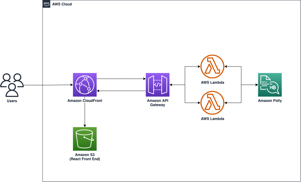
We set up an end-to-end streaming analytics environment, where a Kinesis data stream is ingested with a trimmed-down version of the Amazon Customer Reviews dataset and consumed by a Kinesis Data Analytics Studio notebook powered by Apache Zeppelin. A UDF is attached to the entire notebook instance, which allows the notebook to trigger Amazon Comprehend and Amazon Translate APIs using the payload from the Kinesis data stream. The following diagram illustrates the solution architecture.

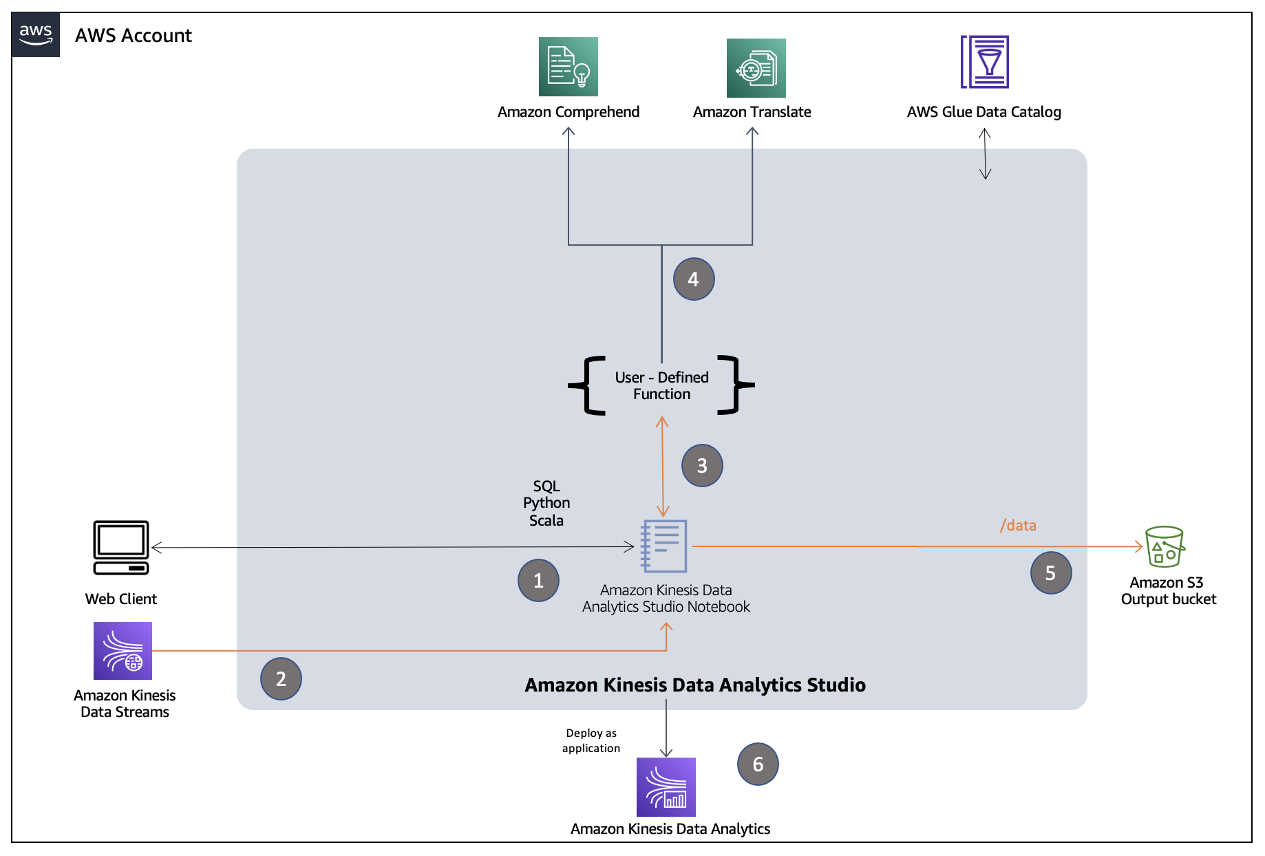
The response from the UDF is used to enrich the payloads from the data stream, which are then stored in an Amazon Simple Storage Service (Amazon S3) bucket. Schema and related metadata are stored in a dedicated AWS Glue Data Catalog. After the results in S3 bucket meet your expectations, the Studio notebook instance is deployed as a Kinesis Data Analytics application for continuous streaming analytics.

How the UDF works

The Java class TextAnalyticsUDF implements the core logic for each of our UDFs. This class extends ScalarFunction to allow invocation from Kinesis Data Analytics for Flink on a per-record basis. The required eval method is then overloaded to receive input records, the identifier for the use case to perform, and other supporting metadata for the use case. A switch case within the eval methods then maps the input record to a corresponding public method. Within these public methods, use case-specific API calls of Amazon Comprehend and Amazon Translate are triggered, for example DetectSentiment, DetectDominantLanguage, and TranslateText.

Amazon Comprehend API service quotas provide guardrails to limit your cost exposure from unintentional high usage (we discuss this more in the following section). By default, the single-document APIs process up to 20 records per second. Our UDFs use exponential backoff and retry to throttle the request rate to stay within these limits. You can request increases to the transactions per-second quota for APIs using the Quota Request Template on the AWS Management Console.

Amazon Comprehend and Amazon Translate each enforce a maximum input string length of 5,000 utf-8 bytes. Text fields that are longer than 5,000 utf-8 bytes are truncated to 5,000 bytes for language and sentiment detection, and split on sentence boundaries into multiple text blocks of under 5,000 bytes for translation and entity or PII detection and redaction. The results are then combined.

Cost involved

In addition to Kinesis Data Analytics costs, the text analytics UDFs incur usage costs from Amazon Comprehend and Amazon Translate. The amount you pay is a factor of the total number of records and characters that you process with the UDFs. For more information, see Amazon Kinesis Data Analytics pricing, Amazon Comprehend pricing, and Amazon Translate pricing.

Example 1: Analyze the language and sentiment of tweets

Let’s assume you have 10,000 tweet records, with an average length of 100 characters per tweet. Your SQL query detects the dominant language and sentiment for each tweet. You’re in your second year of service (the Free Tier no longer applies). The cost details are as follows:

• Size of each tweet = 100 characters
• Number of units (100 character) per record (minimum is 3 units) = 3
• Total units = 10,000 (records) x 3 (units per record) x 2 (Amazon Comprehend requests per record) = 60,000
• Price per unit = $0.0001
• Total cost for Amazon Comprehend = [number of units] x [cost per unit] = 60,000 x $0.0001 = $6.00

Example 2: Translate tweets

Let’s assume that 2,000 of your tweets aren’t in your local language, so you run a second SQL query to translate them. The cost details are as follows:

• Size of each tweet = 100 characters
• Total characters = 2,000 (records) * 100 (characters per record) x 1 (Amazon Translate requests per record) = 200,000
• Price per character = $0.000015
• Total cost for Amazon Translate = [number of characters] x [cost per character] = 200,000 x $0.000015 = $3.00

Deploy solution resources

For this post, we provide an AWS CloudFormation template to create the following resources:

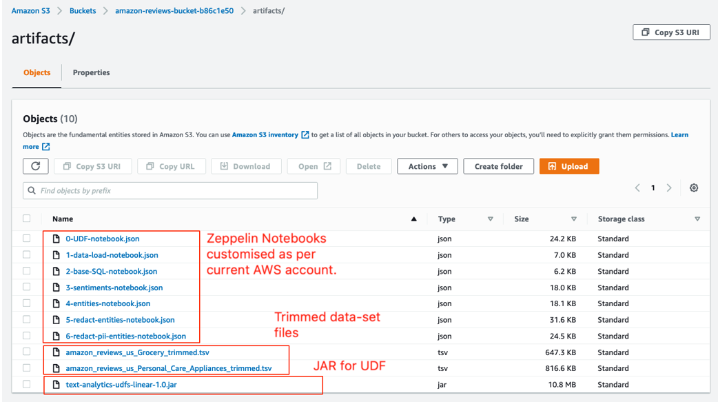
• An S3 bucket named amazon-reviews-bucket-<your-stack-id> that contains artifacts copied from another public S3 bucket outside of your account. These artifacts include:
  • A trimmed-down version of the Amazon Product Review dataset with 2,000 tab-separated reviews of personal care and grocery items. The number of reviews has been reduced to minimize costs of implementing this example.
  • A JAR file to support UDF logic.
• A Kinesis data stream named amazon-kinesis-raw-stream-<your-stack-id> along with a Kinesis Analytics Studio notebook instance named amazon-reviews-studio-application-<your-stack-id> with a dedicated AWS Glue Data Catalog, pre-attached UDF JAR, and a pre-configured S3 path for the deployed application.
• AWS Identity and Access Management (IAM) roles and policies with appropriate permissions.
• AWS Lambda functions for supporting the following operations :
  • Customize Zeppelin notebooks as per the existing stack environment and copy them to the S3 bucket
  • Start the Kinesis Data Analytics Studio instance
  • Modify the CORS policy of the S3 bucket to allow notebook imports via S3 pre-signed URLs
  • Empty the S3 bucket upon stack deletion

To deploy these resources, complete the following steps:

1. Launch the CloudFormation stack:
   
2. Enter a stack name, and leave other parameters at their default.
3. Select I acknowledge that AWS CloudFormation might create IAM resources with custom names.
4. Choose Create stack.
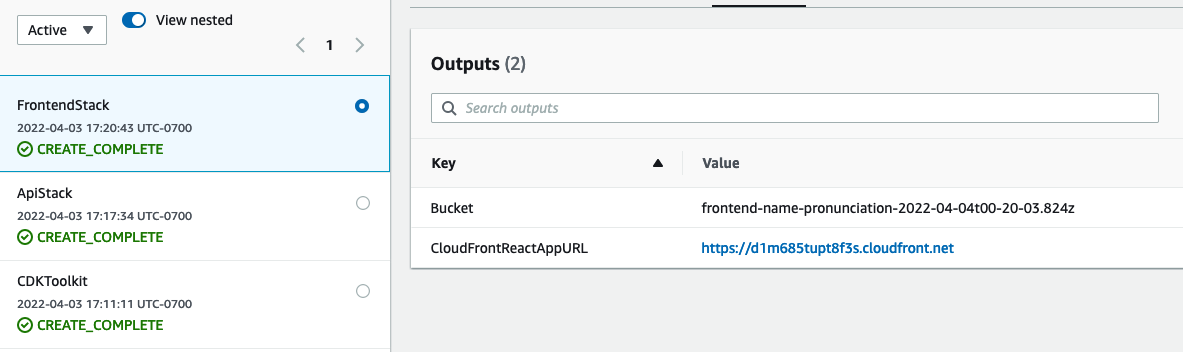
5. When the stack is complete, choose the Outputs tab to review the primary resources created for this solution.
   
6. Copy the S3 bucket name from the Outputs
7. Navigate to the Amazon S3 console in a new browser tab and enter the bucket name in the search bar to filter.
8. Choose the bucket name and list all objects created under the /artifacts/ prefix.

In upcoming steps, we upload these customized Zeppelin notebooks from this S3 bucket to the Kinesis Data Analytics Studio instance via Amazon S3 pre-signed URLs. The import is made possible because the CloudFormation stack attaches a CORS policy on the S3 bucket, which allows the Kinesis Data Analytics Studio instance to perform GET operations. To confirm, navigate to the root prefix of the S3 bucket, choose the Permissions tab, and navigate to the Cross-origin resource sharing (CORS) section.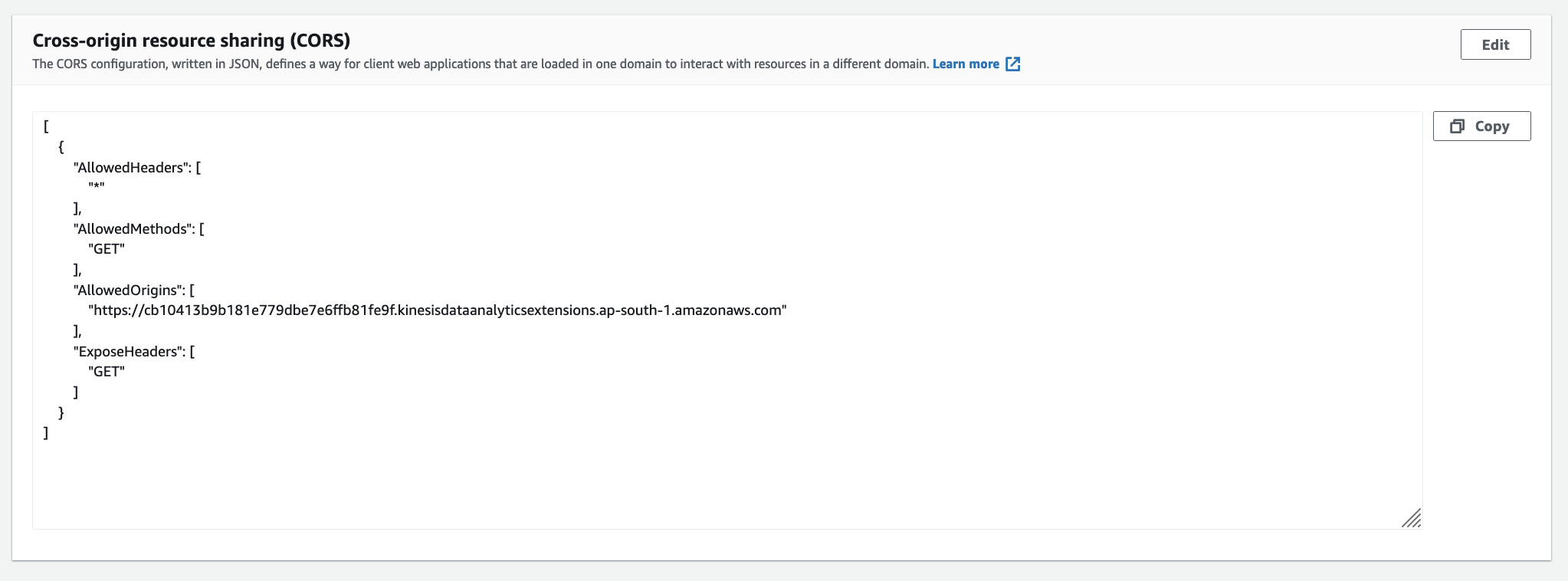

Set up the Studio notebooks

To set up your notebooks, complete the following steps:

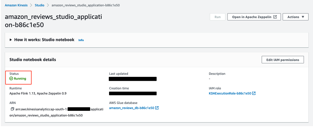
1. On the Kinesis Data Analytics console, choose the Studio tab.
2. Filter for the notebook instance you created and choose the notebook name.
   
3. Confirm that the status shows as Running.
   
4. Choose the Configuration tab and confirm that the application is attached with an S3 path similar to s3://amazon-reviews-bucket-<stack-id>/zeppelin-code/ under Deploy as application configuration.
   This path is used during the export of a notebook to a Kinesis Data Analytics application.
5. Also confirm that an S3 path similar to s3://amazon-reviews-bucket-<stack-id>/artifacts/text-analytics-udfs-linear-1.0.jar exists under User-defined functions.
   This path points the notebook instance towards the UDF JAR.
6. Choose Open in Apache Zeppelin to be redirected to the Zeppelin console.
   

Now you’re ready to import the notebooks to the Studio instance.

7. Open a new browser tab and navigate to your bucket on the Amazon S3 console.
8. Choose the hyperlink for the 0-data-load-notebook.json
   
9. Choose Open.
   
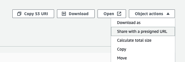
10. Copy the pre-signed URL of the S3 file.
    If your browser doesn’t parse the JSON file in a new tab but downloads the file upon choosing Open, then you can also generate the presigned URL by choosing the Object actions drop-down menu and then Share with a presigned URL.
    
11. On the Zeppelin console, choose Import Note.
12. Choose Add from URL.
    
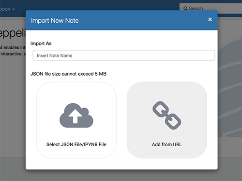
13. Enter the pre-signed URL that you copied.
14. Choose Import Note.
    
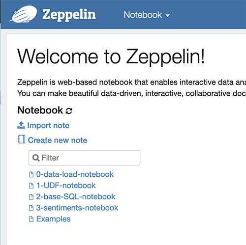
15. Repeat these steps for the remaining notebook files:
    • 1-UDF-notebook.json
    • 2-base-SQL-notebook.json
    • 3-sentiments-notebook.json

The following screenshot shows your view on the Zeppelin console after importing all four files.

For the sake of brevity, this post illustrates a step-by-step walkthrough of the import and run process for the sentiment analysis and language translation use case only. We don’t illustrate the similar processes for 4-entities-notebook, 5-redact-entities-notebook, or 6-redact-pii-entities-notebook in the amazon-reviews-bucket-<your-stack-id> S3 bucket.

That being said, 0-UDF-notebook, 1-data-load-notebook, and 2-base-SQL-notebook are prerequisite resources for all use cases. If you already have the prerequisites set up, these distinct use case notebooks can operate similar to 3-sentiments-notebook. In a later section, we showcase the expected results for these use cases.

Studio notebook structure

To visualize the flow better, we have segregated the separate use cases into individual Studio notebooks. You can download all seven notebooks from the GitHub repo. The following diagram helps illustrate the logical flow for our sentiment detection use case.

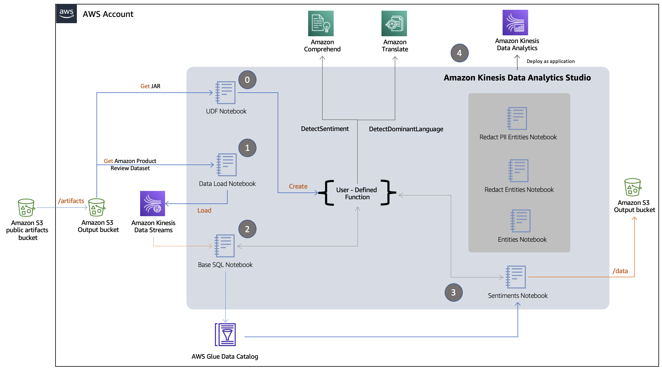
The workflow is as follows:

• Step 0 – The notebook 0-data-load-notebook reads the Amazon Product Review dataset from the local S3 bucket and ingests the tab-separated reviews into a Kinesis data stream.
• Step 1 – The notebook 1-UDF-notebook uses the attached JAR file to create a UDF within StreamTableEnvironment. It also consists of other cells (#4–14) that illustrate UDF usage examples on non-streaming static data.
• Step 2 – The notebook 2-base-SQL-notebook creates a table for the Kinesis data stream in the AWS Glue Data Catalog and uses the language detection and translation capabilities of UDF to enrich the schema with extra columns: review_body_detected_language and review_body_in_french.
• Step 3 – The notebook 3-sentiments-notebook performs the following actions:
  • Step 3.1 – Reads from the table created in Step 2.
  • Step 3.2 – Interacts with the UDF to create views with use case-specific columns (for example, detected_sentiment and sentiment_mixed_score).
  • Step 3.3 – Dumps the streaming data into a local S3 bucket.
• Step 4 – The studio instance saves the notebook as zip export into Amazon S3 bucket which is then used to create a standalone Amazon Kinesis Data Analytics application .

Steps 0–2 are mandatory for the remaining steps to run. Step 3 remains the same for use cases with the other notebooks (4-entities-notebook, 5-redact-entities-notebook, and 6-redact-pii-entities-notebook).

Run Studio notebooks

In this section, we walk through the cells of the following notebooks:

• 0-UDF-notebook
• 1-data-load-notebook
• 2-base-SQL-notebook
• 3-sentiments-notebook

0-data-load-notebook

Cell #1 registers a Flink UDF with StreamTableEnvironment. Choose the play icon at the top of cell to run this cell.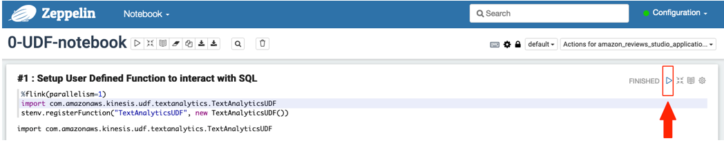Cell #2 enables checkpointing, which is important for allowing S3Sink (used in 3-sentiments-notebook later) to run as expected.

Cells #3–13 are optional for understanding the functionality of UDFs on static non-streaming text. Additionally, the appendix at the end of this post provides a quick walkthrough of the solution capabilities.

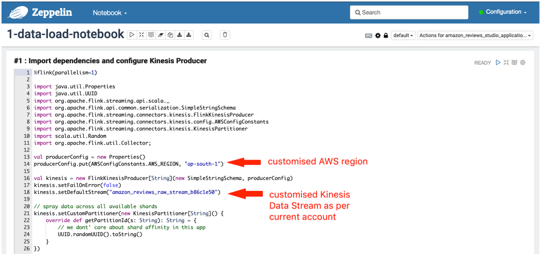
1-data-load-notebook

Choose the play icon at the top of each cell (#1 and #2) to load data into a Kinesis data stream.

Cell #1 imports the dependencies into the runtime and configures the Kinesis producer with Kinesis data stream name and Region for ingestion. The Region and stream name variables are pre-populated as per the AWS account in which the CloudFormation stack was deployed.

Cell #2 loads the trimmed-down version of the Amazon Customer Reviews dataset into the Kinesis data stream.2-base-SQL-notebook

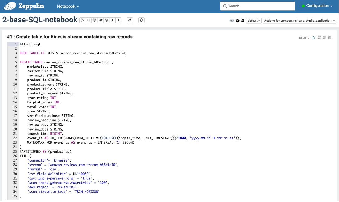
Choose the play icon at the top of each cell (#1 and #2) to run the notebook.

Cell #1 creates a table schema in the AWS Glue Data Catalog for the Kinesis data stream.

Cell #2 creates the view amazon_reviews_enriched on the streaming data and runs the UDF to enrich additional columns in the schema (review_body_in_french and review_body_detected_language).

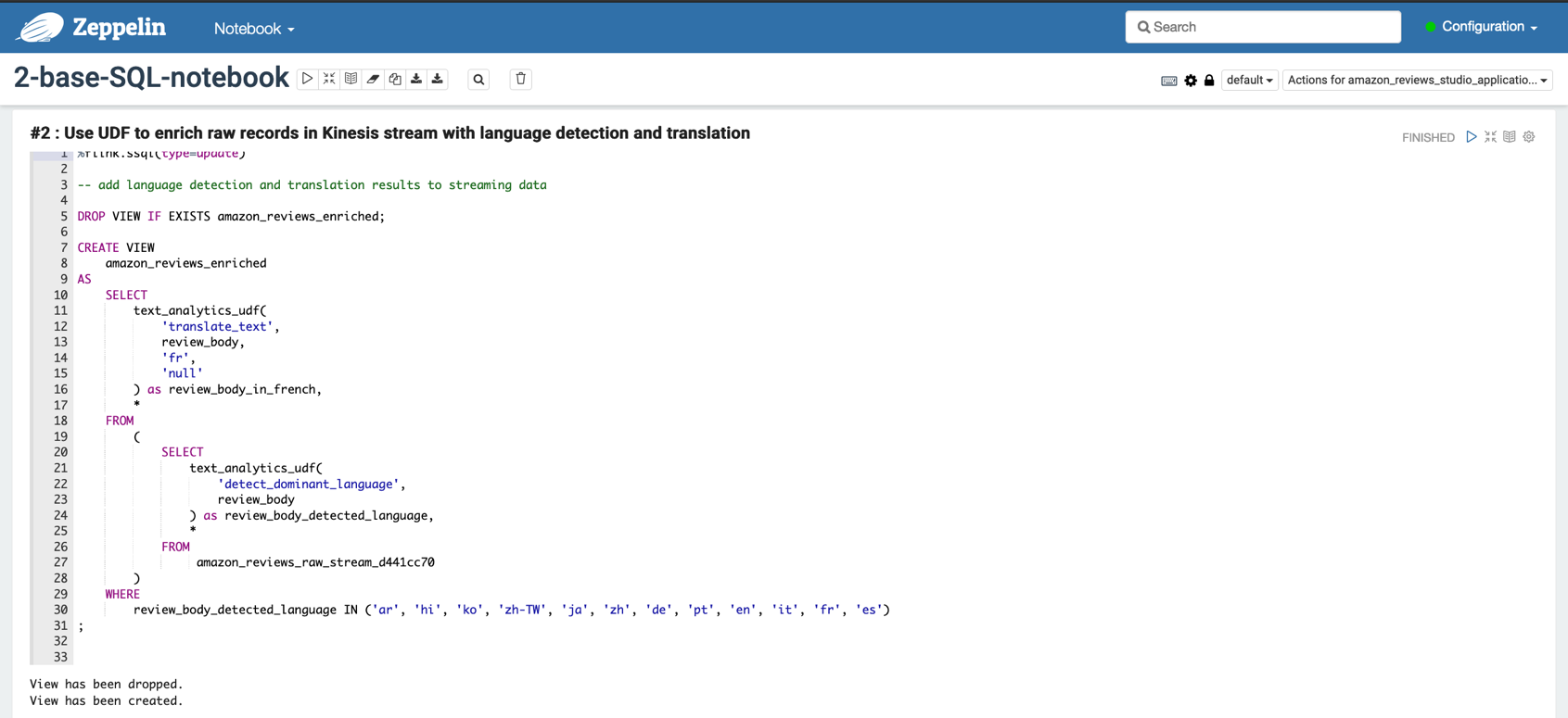
Cell #3 is optional for understanding the modifications on the base schema.

3-sentiments-notebook

Choose the play icon at the top of each cell (#1–3) to run the notebook.

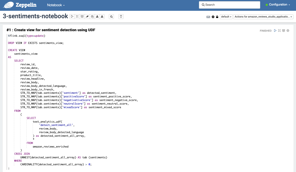
Cell #1 creates another view named sentiment_view on top of the amazon_reviews_enriched view to further determine the sentiments of the product reviews.

Because the intention of cell #2 is to have a quick preview of rows expected in the destination S3 bucket and we don’t need the corresponding Flink job to run forever, choose the cancel icon in cell #2 to stop the job after you get sufficient rows as output. You can expect the notebook cell to populate with results in approximately 2–3 minutes. This duration is a one-time investment to start the Flink job, after which the job continues to process streaming data as it arrives.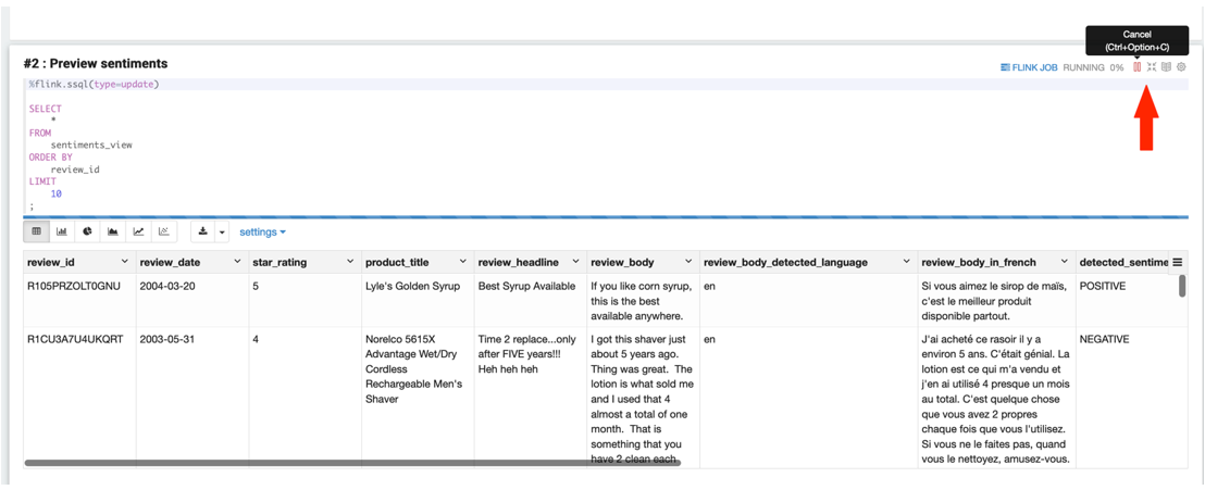

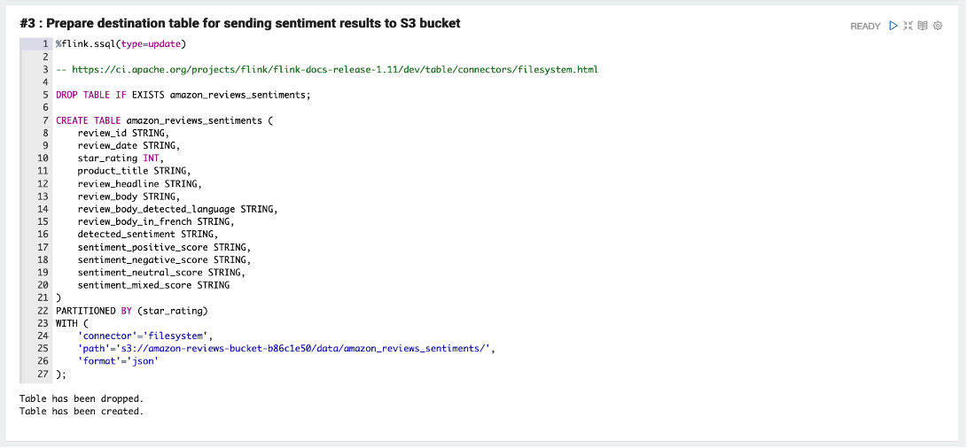
Cell #3 creates a table called amazon_reviews_sentiments to store the UDF modified streaming data in an S3 bucket.

Run cell #4 to send sentiments to the S3 destination bucket. This cell creates an Apache Flink job that reads dataset records from the Kinesis data stream, applies the UDF transformations, and stores the modified records in Amazon S3.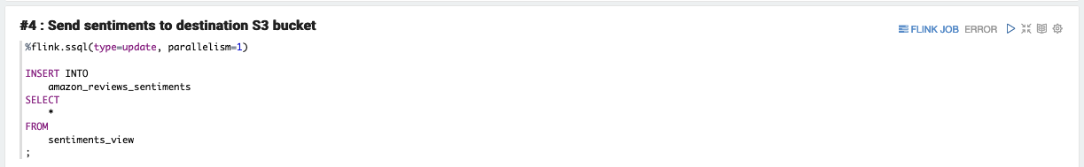

You can expect the notebook cell to populate the S3 bucket with results in approximately 5 minutes. Note, this duration is a one-time investment to start the Flink job, after which the job continues to process streaming data as it arrives. You can stop the notebook cell to stop this Flink job after you review the end results in the S3 bucket.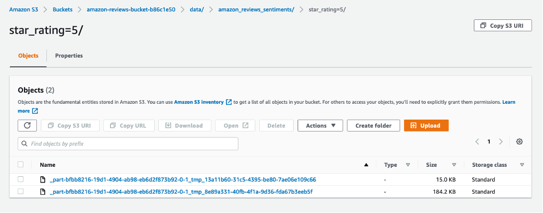

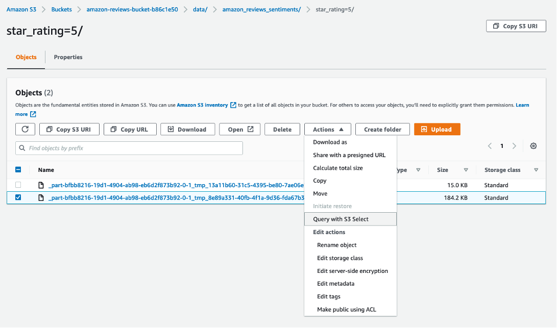
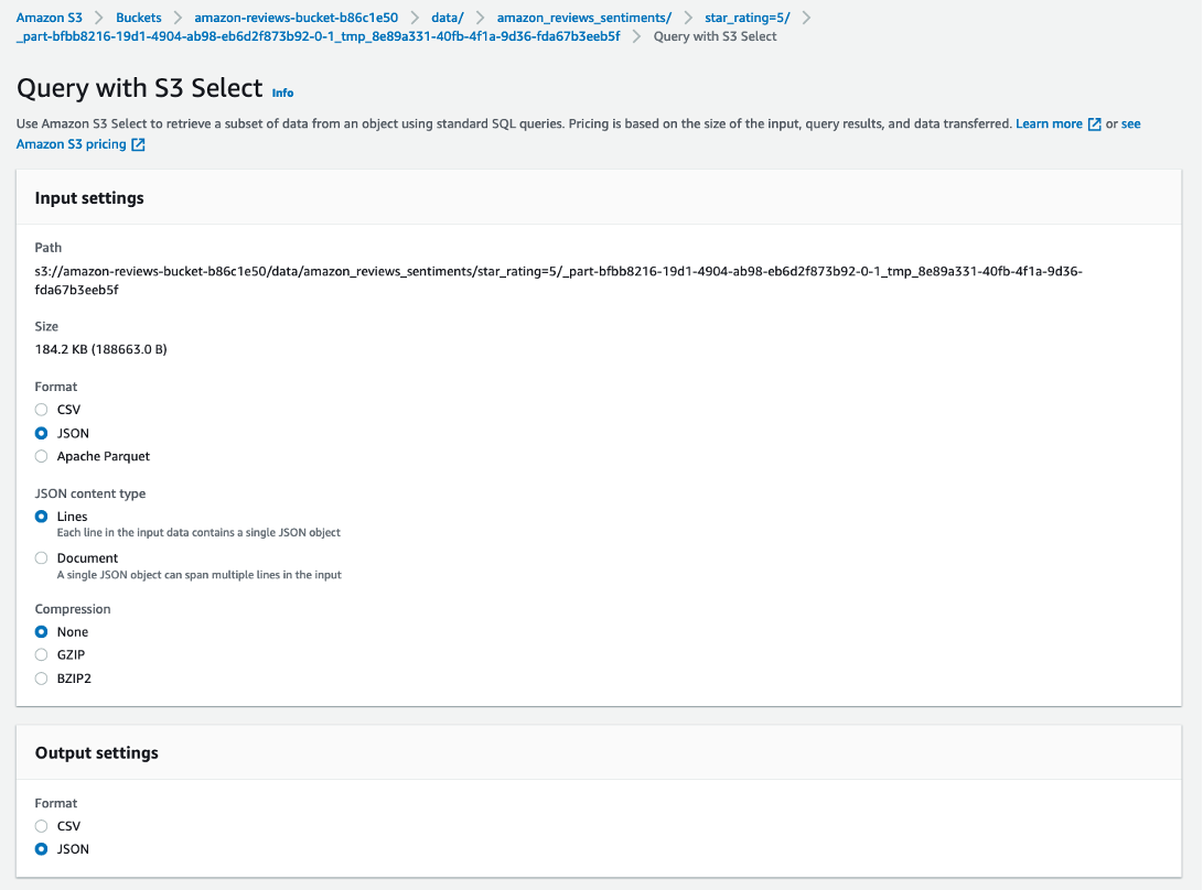
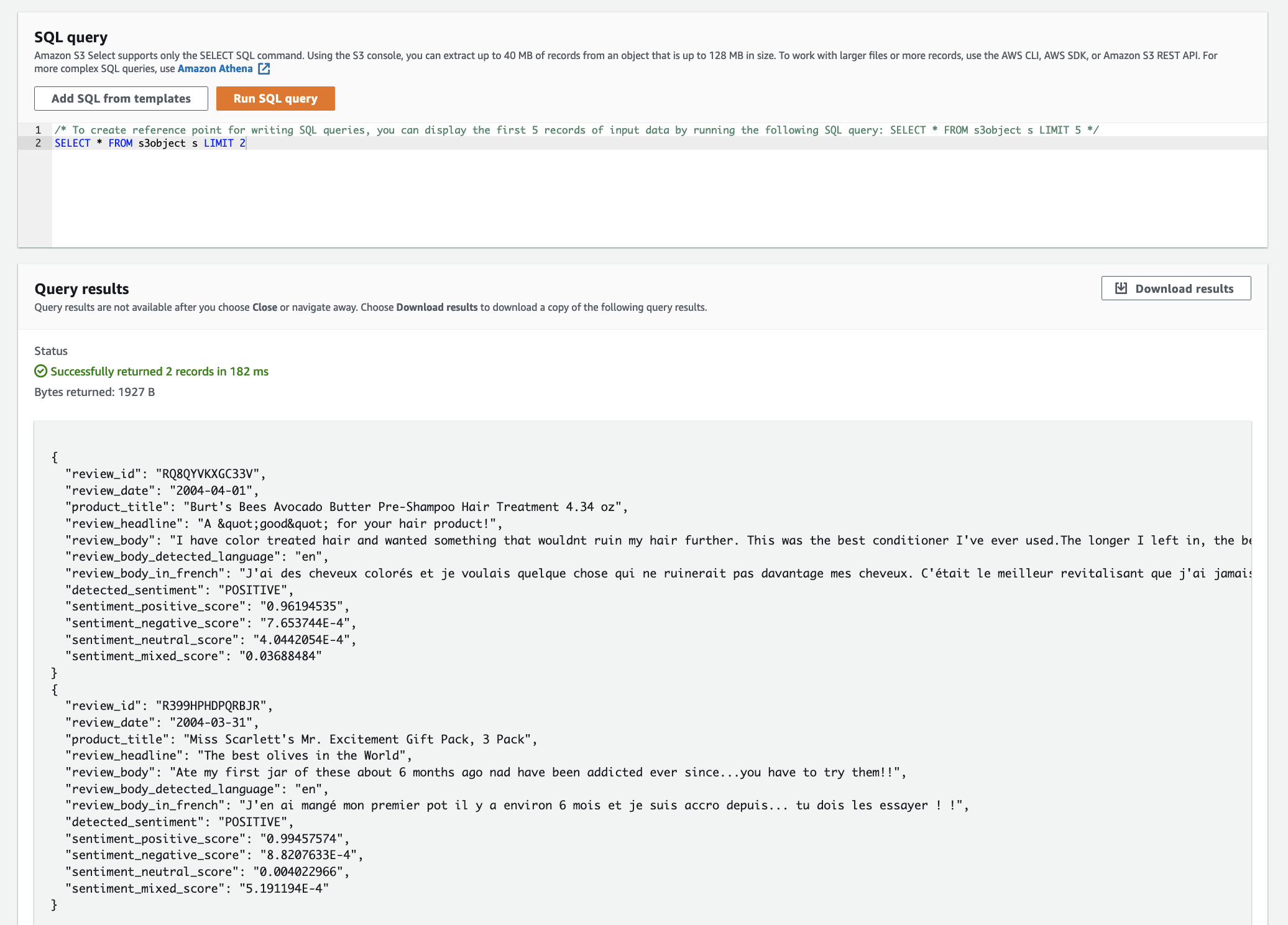
Query the file using S3 Select to validate the contents.

The following screenshot shows your query input and output settings.

The following screenshot shows the query results for sentiment detection.

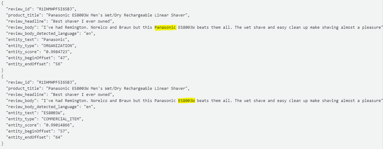
The following are equivalent results of 4-entities-notebook in the S3 bucket.

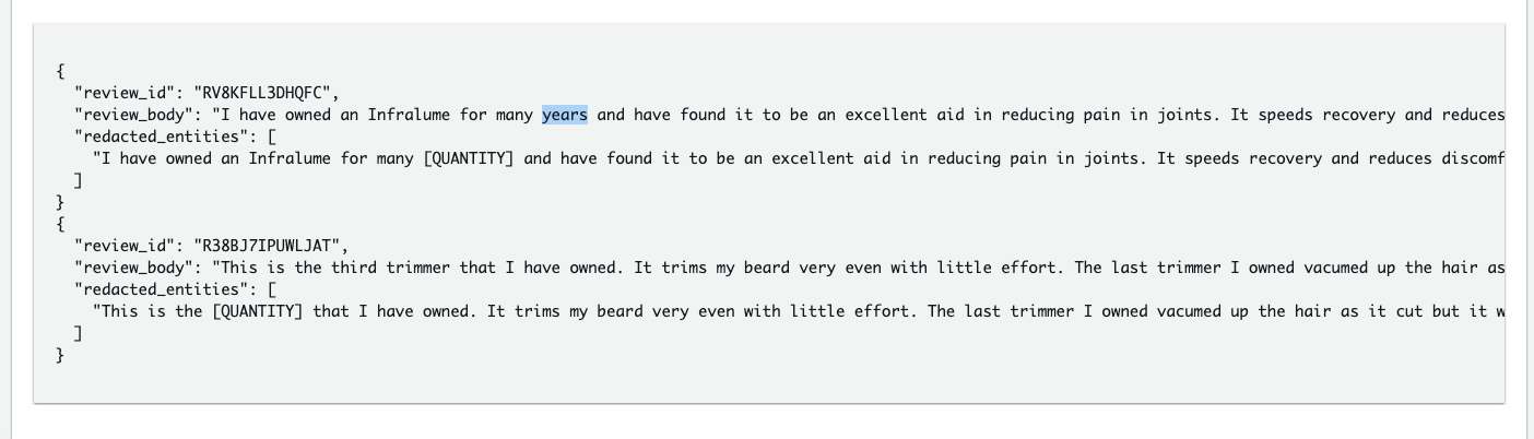
The following are equivalent results of 5-redact-entities-notebook in the S3 bucket.

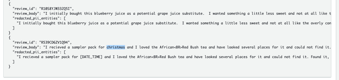
The following are equivalent results of 6-redact-pii-entities-notebook in the S3 bucket.

Export the Studio notebook as a Kinesis Data Analytics application

There are two modes of running an Apache Flink application on Kinesis Data Analytics:

• Create notes within a Studio notebook. This provides the ability to develop your code interactively, view results of your code in real time, and visualize it within your note. We have already achieved this in previous steps.
• Deploy a note to run in streaming mode.

After you deploy a note to run in streaming mode, Kinesis Data Analytics creates an application for you that runs continuously, reads data from your sources, writes to your destinations, maintains a long-running application state, and scales automatically based on the throughput of your source streams.

The CloudFormation stack already configured a Kinesis Data Analytics Studio notebook to store the exported application artifacts in the amazon-reviews-bucket-<your-stack-id>/zeppelin-code/ S3 prefix. The SQL criteria for Studio notebook export prevents the presence of simple SELECT statements in cells of the notebook to export. Therefore, we can’t export 3-sentiments-notebook because the notebook contains SELECT statements under cell #2: Preview sentiments. To export the end result, complete the following steps:

1. Navigate to the Apache Zeppelin UI for the notebook instance.
2. Open 3-sentiments-notebook and copy the last cell’s SQL query:

   %flink.ssql(type=update, parallelism=1)
   INSERT INTO 
       amazon_reviews_sentiments
   SELECT 
       *
   FROM
       sentiments_view;

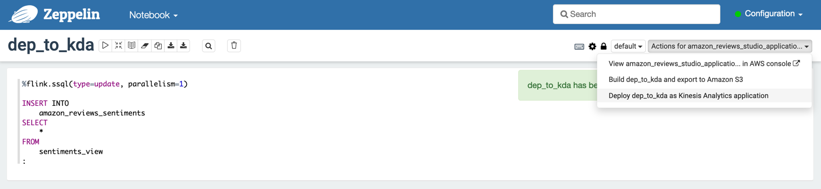
3. Create a new notebook (named dep_to_kda in this post) and enter the copied content into a new cell.
4. On the Actions menu, choose Build and export to Amazon S3.
   
5. Enter an application name, confirm the S3 destination path, and choose Build and export.
   
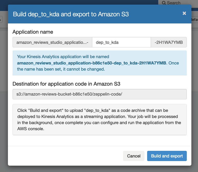
   The process of building and exporting the artifacts is complete in approximately 5 minutes. You can monitor the progress on the console.
   
6. Validate the creation of the required ZIP export in the S3 bucket.
   
7. Navigate back to the Apache Zeppelin UI for the notebook instance and open the newly created notebook (named dep-to-kda in this post).
8. On the Actions menu, choose Deploy export as Kinesis Analytics application.
   
   
9. Choose Deploy using AWS console to continue with the deployment.
   
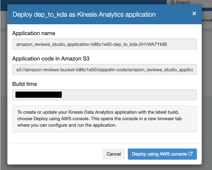
   You’re automatically redirected to the Kinesis Data Analytics console.
10. On the Kinesis Data Analytics console, select Choose from IAM roles that Kinesis Data Analytics can assume and choose the KDAExecutionRole-<stack-id> role.
    
11. Leave the remaining configurations at default and choose Create streaming application.
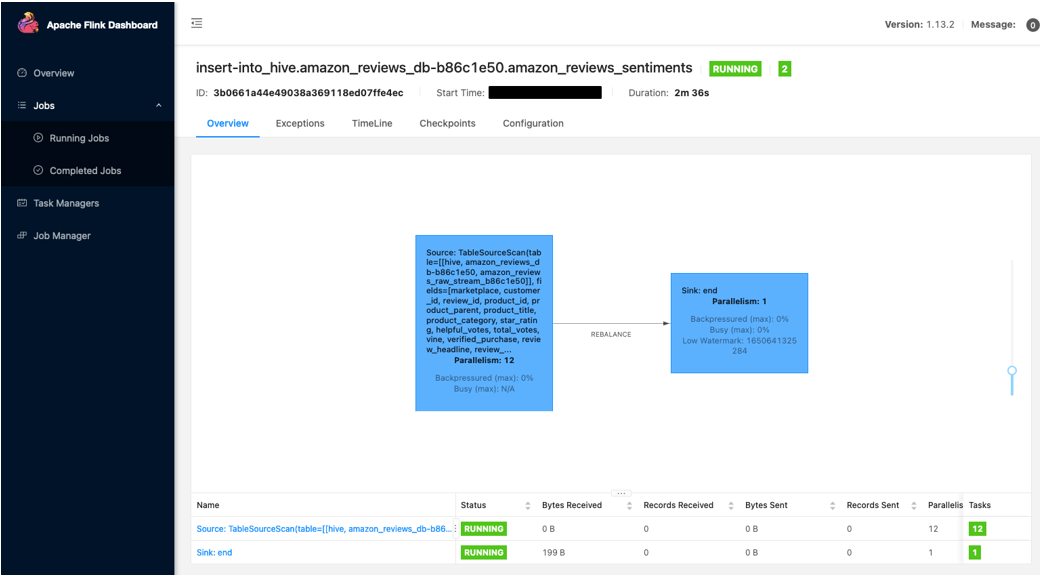
12. Navigate back to the Kinesis Analytics application and choose Run to run the application.
    
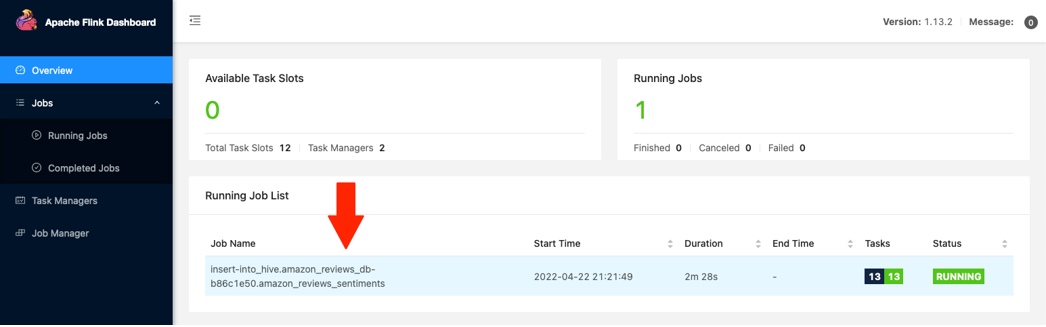
13. When the status shows as Running, choose Open Apache Flink Dashboard.
    

You can now review the progress of the running Flink job.

Troubleshooting

If your query fails, check the Amazon CloudWatch logs generated by the Kinesis Data Analytics for Flink application:

1. On the Kinesis Data Analytics console, choose the exported application in previous steps and navigate to the Configuration
2. Scroll down and choose Logging and Monitoring.
3. Choose the hyperlink under Log Group to open the log streams for additional troubleshooting insights.

For more information about viewing CloudWatch logs, see Logging and Monitoring in Amazon Kinesis Data Analytics for Apache Flink.

Additional use cases

There are many use cases for the discussed text analytics functions. In addition to the example shown in this post, consider the following:

• Prepare research-ready datasets by redacting PII from customer or patient interactions.
• Simplify extract, transform, and load (ETL) pipelines by using incremental SQL queries to enrich text data with sentiment and entities, such as streaming social media streams ingested by Amazon Kinesis Data Firehose.
• Use SQL queries to explore sentiment and entities in your customer support texts, emails, and support cases.
• Standardize many languages to a single common language.

You may have additional use cases for these functions, or additional capabilities you want to see added, such as the following:

• SQL functions to call custom entity recognition and custom classification models in Amazon Comprehend.
• SQL functions for de-identification—extending the entity and PII redaction functions to replace entities with alternate unique identifiers.

The implementation is open source, which means that you can clone the repo, modify and extend the functions as you see fit, and (hopefully) send us pull requests so we can merge your improvements back into the project and make it better for everyone.

Clean up

After you complete this tutorial, you might want to clean up any AWS resources you no longer want to use. Active AWS resources can continue to incur charges in your account.

Because the deployed Kinesis Data Analytics application is independent of the CloudFormation stack, we need to delete the application individually.

1. On the Kinesis Data Analytics console, select the application.
2. On the Actions drop-down menu, choose Delete.
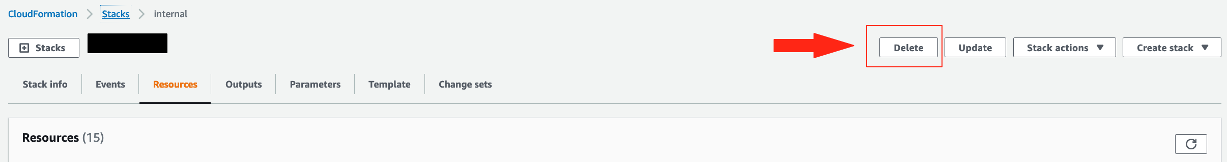
3. On the AWS CloudFormation console, choose the stack deployed earlier and choose Delete.
   

Conclusion

We have shown you how to install the sample text analytics UDF function for Kinesis Data Analytics, so that you can use simple SQL queries to translate text using Amazon Translate, generate insights from text using Amazon Comprehend, and redact sensitive information. We hope you find this useful, and share examples of how you can use it to simplify your architectures and implement new capabilities for your business.

The SQL functions described in this post are also available for Amazon Athena and Amazon Redshift. For more information, see Translate, redact, and analyze text using SQL functions with Amazon Athena, Amazon Translate, and Amazon Comprehend and Translate and analyze text using SQL functions with Amazon Redshift, Amazon Translate, and Amazon Comprehend.

Please share your thoughts with us in the comments section, or in the issues section of the project’s GitHub repository.

Appendix: Available function reference

This section summarizes the example queries and results on non-streaming static data. To access these functions in your CloudFormation deployed environment, refer to cells #3–13 of 0-UDF-notebook.

Detect language

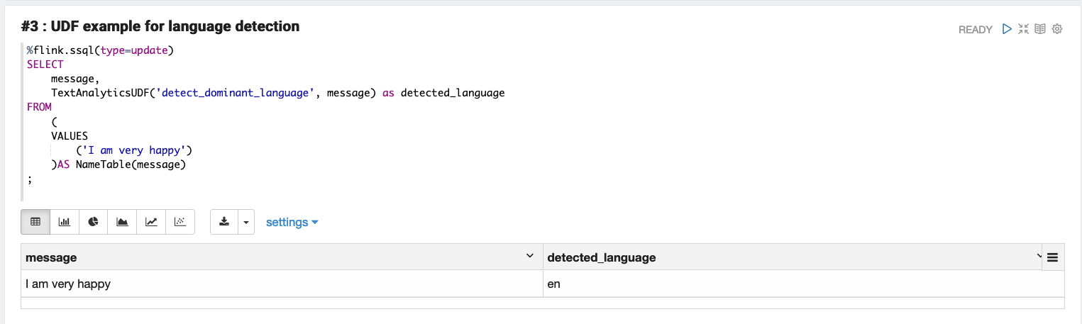
This function uses the Amazon Comprehend DetectDominantLanguage API to identify the dominant language and return a language code, such as fr for French or en for English:

%flink.ssql(type=update)
SELECT
    message,
    TextAnalyticsUDF('detect_dominant_language', message) as detected_language
FROM 
	(
	VALUES
        ('I am very happy')
    )AS NameTable(message)
;

         message     | detected_language
=====================================
I am very happy | en

The following code returns a comma-separated string of language codes and corresponding confidence scores:

%flink.ssql(type=update)
SELECT
    message,
    TextAnalyticsUDF('detect_dominant_language_all', message) as detected_language
FROM 
	(
	VALUES
        ('I am very happy et joyeux')
    )AS NameTable(message)
;

              message     |               detected_language
============================================================================
I am very happy et joyeux | lang_code=fr,score=0.5603816,lang_code=en,score=0.30602336

Detect sentiment

This function uses the Amazon Comprehend DetectSentiment API to identify the sentiment and return results as POSITIVE, NEGATIVE, NEUTRAL, or MIXED:

%flink.ssql(type=update)

SELECT
message,
TextAnalyticsUDF(‘detect_sentiment’, message, ‘en’) as sentiment
FROM 
	(
	VALUES
               (‘I am very happy’)
)AS NameTable(message)
;

    message     | sentiment
================================
I am very happy | [POSITIVE]

The following code returns a comma-separated string containing detected sentiment and confidence scores for each sentiment value:

%flink.ssql(type=update)
SELECT
    message,
    TextAnalyticsUDF('detect_sentiment_all', message, 'en') as sentiment
FROM 
	(
	VALUES
        ('I am very happy')
    )AS NameTable(message)
;

    message     | sentiment
=============================================================================================================================================
I am very happy | [sentiment=POSITIVE,positiveScore=0.999519,negativetiveScore=7.407639E-5,neutralScore=2.7478999E-4,mixedScore=1.3210243E-4]

Detect entities

This function uses the Amazon Comprehend DetectEntities API to identify entities:

%flink.ssql(type=update)
SELECT
    message,
    TextAnalyticsUDF('detect_entities', message, 'en') as entities
FROM 
	(
	VALUES
        ('I am Bob, I live in Herndon VA, and I love cars')
    )AS NameTable(message)
;

		                     message    |              entities
=============================================================================================
I am Bob, I live in Herndon VA, and I love cars | [[["PERSON","Bob"],["LOCATION","Herndon VA"]]]

The following code returns a comma-separated string containing entity types and values:

%flink.ssql(type=update)
SELECT
    message,
    TextAnalyticsUDF('detect_entities_all', message, 'en') as entities
FROM 
	(
	VALUES
        ('I am Bob, I live in Herndon VA, and I love cars')
    )AS NameTable(message)
;

		       message    |              entities
=============================================================================================
I am Bob, I live in Herndon VA, and I love cars |[score=0.9976127,type=PERSON,text=Bob,beginOffset=5,endOffset=8, score=0.995559,type=LOCATION,text=Herndon VA,beginOffset=20,endOffset=30]

Detect PII entities

This function uses the DetectPiiEntities API to identify PII:

%flink.ssql(type=update)
SELECT
    message,
    TextAnalyticsUDF('detect_pii_entities', message, 'en') as pii_entities
FROM 
	(
	VALUES
        ('I am Bob, I live in Herndon VA, and I love cars')
    )AS NameTable(message)
;

		       message    |              pii_entities
=============================================================================================
I am Bob, I live in Herndon VA, and I love cars | [[["NAME","Bob"],["ADDRESS","Herndon VA"]]]

The following code returns a comma-separated string containing PII entity types, with their scores and character offsets:

%flink.ssql(type=update)
SELECT
    message,
    TextAnalyticsUDF('detect_pii_entities_all', message, 'en') as pii_entities
FROM 
	(
	VALUES
        ('I am Bob, I live in Herndon VA, and I love cars')
    )AS NameTable(message)
;


		       message    |              pii_entities
=============================================================================================
I am Bob, I live in Herndon VA, and I love cars | [score=0.9999832,type=NAME,beginOffset=5,endOffset=8, score=0.9999931,type=ADDRESS,beginOffset=20,endOffset=30]

Redact entities

This function replaces entity values for the specified entity types with “[ENTITY_TYPE]”:

%flink.ssql(type=update)
SELECT
    message,
    TextAnalyticsUDF('redact_entities', message, 'en') as redacted_entities
FROM 
	(
	VALUES
        ('I am Bob, I live in Herndon VA, and I love cars')
    )AS NameTable(message)
;
		
				         message                 |              redacted_entities
=====================================================================================================
I am Bob, I live in Herndon VA, and I love cars | [I am [PERSON], I live in [LOCATION], and I love cars]

Redact PII entities

This function replaces PII entity values for the specified entity types with “[PII_ENTITY_TYPE]”:

%flink.ssql(type=update)
SELECT
    message,
    TextAnalyticsUDF('redact_pii_entities', message, 'en') as redacted_pii_entities
FROM 
	(
	VALUES
        ('I am Bob, I live in Herndon VA, and I love cars')
    )AS NameTable(message)
;
		
				         message                 |              redacted_pii_entities
=====================================================================================================
I am Bob, I live in Herndon VA, and I love cars | [I am [NAME], I live in [ADDRESS], and I love cars]

Translate text

This function translates text from the source language to the target language:

%flink.ssql(type=update)
SELECT
message,
TextAnalyticsUDF(‘translate_text’, message, ‘fr’, ‘null’) as translated_text_to_french
FROM 
	(
	VALUES
               (‘It is a beautiful day in neighborhood’)
)AS NameTable(message)
;

                 Message                |         translated_text_to_french
==================================================================================
It is a beautiful day in neighborhood   | C'est une belle journée dans le quartier

About the Authors

Nikhil Khokhar is a Solutions Architect at AWS. He joined AWS in 2016 and specializes in building and supporting data streaming solutions that help customers analyze and get value out of their data. In his free time, he makes use of his 3D printing skills to solve everyday problems.

Bob Strahan is a Principal Solutions Architect in the AWS Language AI Services team.

Read More

Today, we’re excited to announce that Amazon SageMaker now supports the ability to configure Instance Metadata Service Version 2 (IMDSv2) for Notebook Instances, and for administrators to control the minimum version with which end-users create new Notebook Instances. You can now choose IMDSv2 only for your new and existing SageMaker Notebook Instances to take advantage of the latest protection and support provided by IMDSv2.

Instance metadata is data about your instance that you can use to configure or manage the running instance, by providing temporary and frequently rotated credentials that can only be accessed by software running on the instance. IMDS makes metadata about the instance, such as its network and storage, available through a special link-local IP address of 169.254.169.254. You can use IMDS on your SageMaker Notebook Instances, similar to how you would use IMDS on an Amazon Elastic Compute Cloud (Amazon EC2) instance. For detailed documentation, see Instance metadata and user data.

The release of IMDSv2 adds an additional layer of protection using session authentication. With IMDSv2, each session starts with a PUT request to IMDSv2 to get a secure token, with an expiry time, which can be a minimum of 1 second and a maximum of 6 hours. Any subsequent GET request to IMDS must send the resulting token as a header, in order to receive a successful response. When the specified duration expires, a new token is required for future requests.

A sample IMDSv1 call looks like the following code:

curl http://169.254.169.254/latest/meta-data/profile

With IMDSv2, the call looks like the following code:

TOKEN=`curl -X PUT "http://169.254.169.254/latest/api/token" -H "X-aws-ec2-metadata-token-ttl-seconds: 21600"` 

curl http://169.254.169.254/latest/meta-data/profile -H "X-aws-ec2-metadata-token: $TOKEN"

Adopting IMDSv2 and setting it as the minimum version offers various security benefits over IMDSv1. IMDSv2 protects against unrestricted Web Application Firewall (WAF) configurations, open reverse proxies, Server-Side Request Forgery (SSRF) vulnerabilities, and open layer 3 firewalls and NATs that could be used to access the instance metadata. For a detailed comparison, see Add defense in depth against open firewalls, reverse proxies, and SSRF vulnerabilities with enhancements to the EC2 Instance Metadata Service.

In this post, we show you how to configure your SageMaker notebooks with IMDSv2 only support. We also share the support plan for IMDSv1, and how you can enforce IMDSv2 on your notebooks.

What’s new with IMDSv2 support and SageMaker

You can now configure the IMDS version of SageMaker Notebook Instances while creating or updating the instance, which you can do via the SageMaker API or the SageMaker Console, with the minimum IMDS version parameter. The minimum IMDS version specifies the minimum supported version. Setting to a value of 1 allows support for both IMDSv1 and IMDSv2, and setting the minimum version to 2 supports only IMDSv2. With an IMDSv2-only notebook, you can leverage the additional defense in depth that IMDSv2 provides.

We also provide a SageMaker condition key for IAM policies that allows you to restrict the IMDS version for Notebook Instances through the CreateNotebookInstance and UpdateNotebookInstance API calls. Administrators can use this condition key to restrict their end users to creating and/or updating notebooks to support IMDSv2 only. You can add this condition key to the AWS Identity and Access Management (IAM) policy attached to IAM users, roles or groups responsible for creating and updating notebooks.

Additionally, you can also switch between IMDS version configurations using the minimum IMDS version parameter in the SageMaker UpdateNotebookInstance API.

Support for configuring the IMDS version and restricting the IMDS version to v2 only is now available in all AWS Regions in which SageMaker Notebook Instances are available.

Support plan for IMDS versions on SageMaker Notebook Instances

On June 1, 2022, we rolled out support for controlling the minimum version of IMDS to be used with Amazon SageMaker Notebook Instances. All Notebook Instances launched before June 1, 2022 will have the default minimum version set to 1. You will have the option to update the minimum version to 2 using the SageMaker API or the console.

Configure IMDS version on your SageMaker Notebook Instance

You can configure the minimum IMDS version for SageMaker notebook through the AWS SageMaker console (see Create a Notebook Instance), SDK, or the AWS Command Line Interface (AWS CLI). This is an optional configuration, with a default value to set to 1, meaning that the notebook instance will support both IMDSv1 and IMDSv2 calls.

When creating a new notebook instance on the SageMaker console, you now have the option Minimum IMDS version to specify the minimum supported IMDS version, as shown in the following screenshot. If the value is set to 1, both IMDSv1 and IMDSv2 are supported. If the value is set to 2, only IMDSv2 is supported.

You can also edit an existing notebook instance to support IMDSv2 only using the SageMaker console, as shown in the following screenshot.

The default value will remain 1 until 31 August, 2022, and will switch to 2 on 31 August, 2022.

When using the AWS CLI to create a notebook, you can use the MinimumInstanceMetadataServiceVersion parameter to set the minimum supported IMDS version:

   "InstanceMetadataServiceConfiguration": {
      "MinimumInstanceMetadataServiceVersion": "string"
      //Valid Inputs: "1","2"
   }

The following is a sample AWS CLI command to create a notebook instance with IMDSv2 support only:

aws sagemaker create-notebook-instance 
    --region region 
    --notebook-instance-name my-imds-v2-instance 
    --instance-type ml.t3.medium 
    --role-arn sagemaker-execution-role-arn 
    --instance-metadata-service-configuration MinimumInstanceMetadataServiceVersion=2

If you want to update an existing notebook to support IMDSv2 only, you can do it using the UpdateNotebookInstance API:

aws sagemaker update-notebook-instance 
    --region region 
    --notebook-instance-name my-existing-instance-name 
    --instance-metadata-service-configuration MinimumInstanceMetadataServiceVersion=2

Enforce IMDSv2 for all SageMaker Notebook Instances

You can use a condition key to enforce that your users can only create or update Notebook Instances that support IMDSv2 only, to enhance security. You can use this condition key in IAM policies attached to the IAM users, roles or groups responsible for creating and updating the notebooks, or AWS Organizations service control policies.

The following is a sample policy statement that restricts both create and update notebook instance APIs to allow IMDSv2 only:

{
    "Version": "2012-10-17",
    "Statement":
    [
        {
            "Sid": "AllowSagemakerWithIMDSv2Only",
            "Effect": "Allow",
            "Action":
            [
                "sagemaker:CreateNotebookInstance",
                "sagemaker:UpdateNotebookInstance"
            ],
            "Resource": "*",
            "Condition":
            {
                "StringEquals":
                {
                    "sagemaker:MinimumInstanceMetadataServiceVersion": "2"
                }
            }
        }
    ]
}

Conclusion

Today, we announced support for configuring and administratively restricting your Instance Metadata Service (IMDS) version for Notebook Instances. We showed you how to configure the IMDS version for your new and existing notebooks using the SageMaker console and AWS CLI. We also showed you how to administratively restrict IMDS versions using IAM condition keys, and discussed the advantages of supporting IMDSv2 only.

If you have any questions and feedback regarding IMDSv2, please speak to your AWS support contact or post a message in the Amazon EC2 and Amazon SageMaker discussion forums.

About the Authors

Apoorva Gupta is a Software Engineer on the SageMaker Notebooks team. Her focus is on enabling customers to leverage SageMaker more effectively in all aspects of their ML operations. She has been contributing to Amazon SageMaker Notebooks since 2021. In her spare time, she enjoys reading, painting, gardening, cooking and traveling.

Durga Sury is a ML Solutions Architect in the Amazon SageMaker Service SA team. She is passionate about making machine learning accessible to everyone. In her 3 years at AWS, she has helped set up AI/ML platforms for enterprise customers. Prior to AWS, she enabled non-profit and government agencies derive insights from their data to improve education outcomes. When she isn’t working, she loves motorcycle rides, mystery novels, and hikes with her four-year old husky.

Siddhanth Deshpande is an Engineering Manager at Amazon Web Services (AWS). His current focus is building best-in-class managed Machine Learning (ML) infrastructure and tooling services which aim to get customers from “I need to use ML” to “I am using ML successfully” quickly and easily. He has worked for AWS since 2013 in various engineering roles, developing AWS services like Amazon Simple Notification Service, Amazon Simple Queue Service, Amazon EC2, Amazon Pinpoint and Amazon SageMaker. In his spare time, he enjoys spending time with his family, reading, cooking, gardening and travelling the world.

Prashant Pawan Pisipati is a Principal Product Manager at Amazon Web Services (AWS). He has built various products across AWS and Alexa, and is currently focused on helping Machine Learning practitioners be more productive through AWS services.

Edwin Bejarano is a Software Engineer on the SageMaker Notebooks team. He is an Air Force veteran that has been working for Amazon since 2017 with contributions to services like AWS Lambda, Amazon Pinpoint, Amazon Tax Exemption Program, and Amazon SageMaker. In his spare time, he enjoys reading, hiking, biking, and playing video games.

Read More