Building explainability into the components of machine-learning models

Explanation methods that help users understand and trust machine-learning models often describe how much certain features used in the model contribute to its prediction. For example, if a model predicts a patient’s risk of developing cardiac disease, a physician might want to know how strongly the patient’s heart rate data influences that prediction.

But if those features are so complex or convoluted that the user can’t understand them, does the explanation method do any good?

MIT researchers are striving to improve the interpretability of features so decision makers will be more comfortable using the outputs of machine-learning models. Drawing on years of field work, they developed a taxonomy to help developers craft features that will be easier for their target audience to understand.

“We found that out in the real world, even though we were using state-of-the-art ways of explaining machine-learning models, there is still a lot of confusion stemming from the features, not from the model itself,” says Alexandra Zytek, an electrical engineering and computer science PhD student and lead author of a paper introducing the taxonomy.

To build the taxonomy, the researchers defined properties that make features interpretable for five types of users, from artificial intelligence experts to the people affected by a machine-learning model’s prediction. They also offer instructions for how model creators can transform features into formats that will be easier for a layperson to comprehend.

They hope their work will inspire model builders to consider using interpretable features from the beginning of the development process, rather than trying to work backward and focus on explainability after the fact.

MIT co-authors include Dongyu Liu, a postdoc; visiting professor Laure Berti-Équille, research director at IRD; and senior author Kalyan Veeramachaneni, principal research scientist in the Laboratory for Information and Decision Systems (LIDS) and leader of the Data to AI group. They are joined by Ignacio Arnaldo, a principal data scientist at Corelight. The research is published in the June edition of the Association for Computing Machinery Special Interest Group on Knowledge Discovery and Data Mining’s peer-reviewed Explorations Newsletter.

Real-world lessons

Features are input variables that are fed to machine-learning models; they are usually drawn from the columns in a dataset. Data scientists typically select and handcraft features for the model, and they mainly focus on ensuring features are developed to improve model accuracy, not on whether a decision-maker can understand them, Veeramachaneni explains.

For several years, he and his team have worked with decision makers to identify machine-learning usability challenges. These domain experts, most of whom lack machine-learning knowledge, often don’t trust models because they don’t understand the features that influence predictions.

For one project, they partnered with clinicians in a hospital ICU who used machine learning to predict the risk a patient will face complications after cardiac surgery. Some features were presented as aggregated values, like the trend of a patient’s heart rate over time. While features coded this way were “model ready” (the model could process the data), clinicians didn’t understand how they were computed. They would rather see how these aggregated features relate to original values, so they could identify anomalies in a patient’s heart rate, Liu says.

By contrast, a group of learning scientists preferred features that were aggregated. Instead of having a feature like “number of posts a student made on discussion forums” they would rather have related features grouped together and labeled with terms they understood, like “participation.”

“With interpretability, one size doesn’t fit all. When you go from area to area, there are different needs. And interpretability itself has many levels,” Veeramachaneni says.

The idea that one size doesn’t fit all is key to the researchers’ taxonomy. They define properties that can make features more or less interpretable for different decision makers and outline which properties are likely most important to specific users.

For instance, machine-learning developers might focus on having features that are compatible with the model and predictive, meaning they are expected to improve the model’s performance.

On the other hand, decision makers with no machine-learning experience might be better served by features that are human-worded, meaning they are described in a way that is natural for users, and understandable, meaning they refer to real-world metrics users can reason about.

“The taxonomy says, if you are making interpretable features, to what level are they interpretable? You may not need all levels, depending on the type of domain experts you are working with,” Zytek says.

Putting interpretability first

The researchers also outline feature engineering techniques a developer can employ to make features more interpretable for a specific audience.

Feature engineering is a process in which data scientists transform data into a format machine-learning models can process, using techniques like aggregating data or normalizing values. Most models also can’t process categorical data unless they are converted to a numerical code. These transformations are often nearly impossible for laypeople to unpack.

Creating interpretable features might involve undoing some of that encoding, Zytek says. For instance, a common feature engineering technique organizes spans of data so they all contain the same number of years. To make these features more interpretable, one could group age ranges using human terms, like infant, toddler, child, and teen. Or rather than using a transformed feature like average pulse rate, an interpretable feature might simply be the actual pulse rate data, Liu adds.

“In a lot of domains, the tradeoff between interpretable features and model accuracy is actually very small. When we were working with child welfare screeners, for example, we retrained the model using only features that met our definitions for interpretability, and the performance decrease was almost negligible,” Zytek says.

Building off this work, the researchers are developing a system that enables a model developer to handle complicated feature transformations in a more efficient manner, to create human-centered explanations for machine-learning models. This new system will also convert algorithms designed to explain model-ready datasets into formats that can be understood by decision makers.

Read More

Use a custom image to bring your own development environment to RStudio on Amazon SageMaker

RStudio on Amazon SageMaker is the industry’s first fully managed RStudio Workbench in cloud. You can quickly launch the familiar RStudio integrated development environment (IDE), and dial up and down the underlying compute resources without interrupting your work, making it easy to build machine learning (ML) and analytics solutions in R at scale. RStudio on SageMaker already comes with a built-in image preconfigured with R programming and data science tools; however, you often need to customize your IDE environment. Starting today, you can bring your own custom image with packages and tools of your choice, and make them available to all the users of RStudio on SageMaker in a few clicks.

Bringing your own custom image has several benefits. You can standardize and simplify the getting started experience for data scientists and developers by providing a starter image, preconfigure the drivers required for connecting to data stores, or pre-install specialized data science software for your business domain. Furthermore, organizations that have previously hosted their own RStudio Workbench may have existing containerized environments that they want to continue to use in RStudio on SageMaker.

In this post, we share step-by-step instructions to create a custom image and bring it to RStudio on SageMaker using the AWS Management Console or AWS Command Line Interface (AWS CLI). You can get your first custom IDE environment up and running in few simple steps. For more information on the content discussed in this post, refer to Bring your own RStudio image.

Solution overview

When a data scientist starts a new session in RStudio on SageMaker, a new on-demand ML compute instance is provisioned and a container image that defines the runtime environment (operating system, libraries, R versions, and so on) is run on the ML instance. You can provide your data scientists multiple choices for the runtime environment by creating custom container images and making them available on the RStudio Workbench launcher, as shown in the following screenshot.

The following diagram describes the process to bring your custom image. First you build a custom container image from a Dockerfile and push it to a repository in Amazon Elastic Container Registry (Amazon ECR). Next, you create a SageMaker image that points to the container image in Amazon ECR, and attach that image to your SageMaker domain. This makes the custom image available for launching a new session in RStudio.

Prerequisites

To implement this solution, you must have the following prerequisites:

We provide more details on each in this section.

RStudio on SageMaker domain

If you have an existing SageMaker domain with RStudio enabled prior to April 7, 2022, you must delete and recreate the RStudioServerPro app under the user profile name domain-shared to get the latest updates for bring your own custom image capability. The AWS CLI commands are as follows. Note that this action interrupts RStudio users on SageMaker.

aws sagemaker delete-app 
    --domain-id <sagemaker-domain-id> 
    --app-type RStudioServerPro 
    --app-name default 
    --user-profile-name domain-shared
aws sagemaker create-app 
    --domain-id <sagemaker-domain-id> 
    --app-type RStudioServerPro 
    --app-name default 
    --user-profile-name domain-shared

If this is your first time using RStudio on SageMaker, follow the step-by-step setup process described in Get started with RStudio on Amazon SageMaker, or run the following AWS CloudFormation template to set up your first RStudio on SageMaker domain. If you already have a working RStudio on SageMaker domain, you can skip this step.

The following RStudio on SageMaker CloudFormation template requires an RStudio license approved through AWS License Manager. For more about licensing, refer to RStudio license. Also note that only one SageMaker domain is permitted per AWS Region, so you’ll need to use an AWS account and Region that doesn’t have an existing domain.

  1. Choose Launch Stack.
    Launch stack button
    The link takes you to the us-east-1 Region, but you can change to your preferred Region.
  2. In the Specify template section, choose Next.
  3. In the Specify stack details section, for Stack name, enter a name.
  4. For Parameters, enter a SageMaker user profile name.
  5. Choose Next.
  6. In the Configure stack options section, choose Next.
  7. In the Review section, select I acknowledge that AWS CloudFormation might create IAM resources and choose Next.
  8. When the stack status changes to CREATE_COMPLETE, go to the Control Panel on the SageMaker console to find the domain and the new user.

IAM policies to interact with Amazon ECR

To interact with your private Amazon ECR repositories, you need the following IAM permissions in the IAM user or role you’ll use to build and push Docker images:

{ 
    "Version":"2012-10-17", 
    "Statement":[ 
        {
            "Sid": "VisualEditor0",
            "Effect":"Allow", 
            "Action":[ 
                "ecr:CreateRepository", 
                "ecr:BatchGetImage", 
                "ecr:CompleteLayerUpload", 
                "ecr:DescribeImages", 
                "ecr:DescribeRepositories", 
                "ecr:UploadLayerPart", 
                "ecr:ListImages", 
                "ecr:InitiateLayerUpload", 
                "ecr:BatchCheckLayerAvailability", 
                "ecr:PutImage" 
            ], 
            "Resource": "*" 
        }
    ]
}

To initially build from a public Amazon ECR image as shown in this post, you need to attach the AWS-managed AmazonElasticContainerRegistryPublicReadOnly policy to your IAM user or role as well.

To build a Docker container image, you can use either a local Docker client or the SageMaker Docker Build CLI tool from a terminal within RStudio on SageMaker. For the latter, follow the prerequisites in Using the Amazon SageMaker Studio Image Build CLI to build container images from your Studio notebooks to set up the IAM permissions and CLI tool.

AWS CLI versions

There are minimum version requirements for the AWS CLI tool to run the commands mentioned in this post. Make sure to upgrade AWS CLI on your terminal of choice:

  • AWS CLI v1 >= 1.23.6
  • AWS CLI v2 >= 2.6.2

Prepare a Dockerfile

You can customize your runtime environment in RStudio in a Dockerfile. Because the customization depends on your use case and requirements, we show you the essentials and the most common customizations in this example. You can download the full sample Dockerfile.

Install RStudio Workbench session components

The most important software to install in your custom container image is RStudio Workbench. We download from the public S3 bucket hosted by RStudio PBC. There are many version releases and OS distributions for use. The version of the installation needs to be compatible with the RStudio Workbench version used in RStudio on SageMaker, which is 1.4.1717-3 at the time of writing. The OS (argument OS in the following snippet) needs to match the base OS used in the container image. In our sample Dockerfile, the base image we use is Amazon Linux 2 from an AWS-managed public Amazon ECR repository. The compatible RStudio Workbench OS is centos7.

FROM public.ecr.aws/amazonlinux/amazonlinux
...
ARG RSW_VERSION=1.4.1717-3
ARG RSW_NAME=rstudio-workbench-rhel
ARG OS=centos7
ARG RSW_DOWNLOAD_URL=https://s3.amazonaws.com/rstudio-ide-build/server/${OS}/x86_64
RUN RSW_VERSION_URL=`echo -n "${RSW_VERSION}" | sed 's/+/-/g'` 
    && curl -o rstudio-workbench.rpm ${RSW_DOWNLOAD_URL}/${RSW_NAME}-${RSW_VERSION_URL}-x86_64.rpm 
    && yum install -y rstudio-workbench.rpm

You can find all the OS release options with the following command:

aws s3 ls s3://rstudio-ide-build/server/

Install R (and versions of R)

The runtime for your custom RStudio container image needs at least one version of R. We can first install a version of R and make it the default R by creating soft links to /usr/local/bin/:

# Install main R version
ARG R_VERSION=4.1.3
RUN curl -O https://cdn.rstudio.com/r/centos-7/pkgs/R-${R_VERSION}-1-1.x86_64.rpm && 
    yum install -y R-${R_VERSION}-1-1.x86_64.rpm && 
    yum clean all && 
    rm -rf R-${R_VERSION}-1-1.x86_64.rpm

RUN ln -s /opt/R/${R_VERSION}/bin/R /usr/local/bin/R && 
    ln -s /opt/R/${R_VERSION}/bin/Rscript /usr/local/bin/Rscript

Data scientists often need multiple versions of R so that they can easily switch between projects and code base. RStudio on SageMaker supports easy switching between R versions, as shown in the following screenshot.

RStudio on SageMaker automatically scans and discovers versions of R in the following directories:

/usr/lib/R
/usr/lib64/R
/usr/local/lib/R
/usr/local/lib64/R
/opt/local/lib/R
/opt/local/lib64/R
/opt/R/*
/opt/local/R/*

We can install more versions in the container image, as shown in the following snippet. They will be installed in /opt/R/.

RUN curl -O https://cdn.rstudio.com/r/centos-7/pkgs/R-4.0.5-1-1.x86_64.rpm && 
    yum install -y R-4.0.5-1-1.x86_64.rpm && 
    yum clean all && 
    rm -rf R-4.0.5-1-1.x86_64.rpm

RUN curl -O https://cdn.rstudio.com/r/centos-7/pkgs/R-3.6.3-1-1.x86_64.rpm && 
    yum install -y R-3.6.3-1-1.x86_64.rpm && 
    yum clean all && 
    rm -rf R-3.6.3-1-1.x86_64.rpm

RUN curl -O https://cdn.rstudio.com/r/centos-7/pkgs/R-3.5.3-1-1.x86_64.rpm && 
    yum install -y R-3.5.3-1-1.x86_64.rpm && 
    yum clean all && 
    rm -rf R-3.5.3-1-1.x86_64.rpm

Install RStudio Professional Drivers

Data scientists often need to access data from sources such as Amazon Athena and Amazon Redshift within RStudio on SageMaker. You can do so using RStudio Professional Drivers and RStudio Connections. Make sure you install the relevant libraries and drivers as shown in the following snippet:

# Install RStudio Professional Drivers ----------------------------------------#
RUN yum update -y && 
    yum install -y unixODBC unixODBC-devel && 
    yum clean all

ARG DRIVERS_VERSION=2021.10.0-1
RUN curl -O https://drivers.rstudio.org/7C152C12/installer/rstudio-drivers-${DRIVERS_VERSION}.el7.x86_64.rpm && 
    yum install -y rstudio-drivers-${DRIVERS_VERSION}.el7.x86_64.rpm && 
    yum clean all && 
    rm -f rstudio-drivers-${DRIVERS_VERSION}.el7.x86_64.rpm && 
    cp /opt/rstudio-drivers/odbcinst.ini.sample /etc/odbcinst.ini

RUN /opt/R/${R_VERSION}/bin/R -e 'install.packages("odbc", repos="https://packagemanager.rstudio.com/cran/__linux__/centos7/latest")'

Install custom libraries

You can also install additional R and Python libraries so that data scientists don’t need to install them on the fly:

RUN /opt/R/${R_VERSION}/bin/R -e 
    "install.packages(c('reticulate', 'readr', 'curl', 'ggplot2', 'dplyr', 'stringr', 'fable', 'tsibble', 'dplyr', 'feasts', 'remotes', 'urca', 'sodium', 'plumber', 'jsonlite'), repos='https://packagemanager.rstudio.com/cran/__linux__/centos7/latest')"
    
RUN /opt/python/${PYTHON_VERSION}/bin/pip install --upgrade 
        'boto3>1.0<2.0' 
        'awscli>1.0<2.0' 
        'sagemaker[local]<3' 
        'sagemaker-studio-image-build' 
        'numpy'

When you’ve finished your customization in a Dockerfile, it’s time to build a container image and push it to Amazon ECR.

Build and push to Amazon ECR

You can build a container image from the Dockerfile from a terminal where the Docker engine is installed, such as your local terminal or AWS Cloud9. If you’re building it from a terminal within RStudio on SageMaker, you can use SageMaker Studio Image Build. We demonstrate the steps for both approaches.

In a local terminal where the Docker engine is present, you can run the following commands from where the Dockerfile is. You can use the sample script create-and-update-image.sh.

IMAGE_NAME=r-4.1.3-rstudio-1.4.1717-3           # the name for SageMaker Image
REPO=rstudio-custom                             # ECR repository name
TAG=$IMAGE_NAME
# login to your Amazon ECR
aws ecr get-login-password | docker login --username AWS --password-stdin ${ACCOUNT_ID}.dkr.ecr.${REGION}.amazonaws.com

# create a repo
aws ecr create-repository --repository-name ${REPO}

# build a docker image and push it to the repo
docker build . -t ${REPO}:${TAG} -t ${ACCOUNT_ID}.dkr.ecr.${REGION}.amazonaws.com/${REPO}:${TAG}
docker push ${ACCOUNT_ID}.dkr.ecr.${REGION}.amazonaws.com/${REPO}:${TAG}

In a terminal on RStudio on SageMaker, run the following commands:

pip install sagemaker-studio-image-build
sm-docker build . --repository ${REPO}:${IMAGE_NAME}

After these commands, you have a repository and a Docker container image in Amazon ECR for our next step, in which we attach the container image for use in RStudio on SageMaker. Note the image URI in Amazon ECR <ACCOUNT_ID>.dkr.ecr.<REGION>.amazonaws.com/<REPO>:<TAG> for later use.

Update RStudio on SageMaker through the console

RStudio on SageMaker allows runtime customization through the use of a custom SageMaker image. A SageMaker image is a holder for a set of SageMaker image versions. Each image version represents a container image that is compatible with RStudio on SageMaker and stored in an Amazon ECR repository. To make a custom SageMaker image available to all RStudio users within a domain, you can attach the image to the domain following the steps in this section.

  1. On the SageMaker console, navigate to the Custom SageMaker Studio images attached to domain page, and choose Attach image.
  2. Select New image, and enter your Amazon ECR image URI.
  3. Choose Next.
  4. In the Image properties section, provide an Image name (required), Image display name (optional), Description (optional), IAM role, and tags.
    The image display name, if provided, is shown in the session launcher in RStudio on SageMaker. If the Image display name field is left empty, the image name is shown in RStudio on SageMaker instead.
  5. Leave EFS mount path and Advanced configuration (User ID and Group ID) as default because RStudio on SageMaker manages the configuration for us.
  6. In the Image type section, select RStudio image.
  7. Choose Submit.

You can now see a new entry in the list. It’s worth noting that, with the introduction of the support of custom RStudio images, you can see a new Usage type column in the table to denote whether an image is an RStudio image or an Amazon SageMaker Studio image.

It may take up to 5–10 minutes for the custom images to be available in the session launcher UI. You can then launch a new R session in RStudio on SageMaker with your custom images.

Over time, you may want to retire old and outdated images. To remove the custom images from the list of custom images in RStudio, select the images in the list and choose Detach.

Choose Detach again to confirm.

Update RStudio on SageMaker via the AWS CLI

The following sections describe the steps to create a SageMaker image and attach it for use in RStudio on SageMaker on the SageMaker console and using the AWS CLI. You can use the sample script create-and-update-image.sh.

Create the SageMaker image and image version

The first step is to create a SageMaker image from the custom container image in Amazon ECR by running the following two commands:

ROLE_ARN=<execution-role-that-has-AmazonSageMakerFullAccess-policy>
DISPLAY_NAME=RSession-r-4.1.3-rstudio-1.4.1717-3
aws sagemaker create-image 
    --image-name ${IMAGE_NAME} 
    --display-name ${DISPLAY_NAME} 
    --role-arn ${ROLE_ARN}

aws sagemaker create-image-version 
    --image-name ${IMAGE_NAME} 
    --base-image "${ACCOUNT_ID}.dkr.ecr.${REGION}.amazonaws.com/${REPO}:${TAG}"

Note that the custom image displayed in the session launcher in RStudio on SageMaker is determined by the input of --display-name. If the optional display name is not provided, the input of --image-name is used instead. Also note that the IAM role allows SageMaker to attach an Amazon ECR image to RStudio on SageMaker.

Create an AppImageConfig

In addition to a SageMaker image, which captures the image URI from Amazon ECR, an app image configuration (AppImageConfig) is required for use in a SageMaker domain. We simplify the configuration for an RSessionApp image so we can just create a placeholder configuration with the following command:

IMAGE_CONFIG_NAME=r-4-1-3-rstudio-1-4-1717-3
aws sagemaker create-app-image-config 
    --app-image-config-name ${IMAGE_CONFIG_NAME}

Attach to a SageMaker domain

With the SageMaker image and the app image configuration created, we’re ready to attach the custom container image to the SageMaker domain. To make a custom SageMaker image available to all RStudio users within a domain, you attach the image to the domain as a default user setting. All existing users and any new users will be able to use the custom image.

For better readability, we place the following configuration into the JSON file default-user-settings.json:

    "DefaultUserSettings": {
        "RSessionAppSettings": {
           "CustomImages": [
                {
                     "ImageName": "r-4.1.3-rstudio-2022",
                     "AppImageConfigName": "r-4-1-3-rstudio-2022"
                },
                {
                     "ImageName": "r-4.1.3-rstudio-1.4.1717-3",
                     "AppImageConfigName": "r-4-1-3-rstudio-1-4-1717-3"
                }
            ]
        }
    }
}

In this file, we can specify the image and AppImageConfig name pairs in a list in DefaultUserSettings.RSessionAppSettings.CustomImages. This preceding snippet assumes two custom images are being created.

Then run the following command to update the SageMaker domain:

aws sagemaker update-domain 
    --domain-id <sagemaker-domain-id> 
    --cli-input-json file://default-user-settings.json

After you update the domaim, it may take up to 5–10 minutes for the custom images to be available in the session launcher UI. You can then launch a new R session in RStudio on SageMaker with your custom images.

Detach images from a SageMaker domain

You can detach images simply by removing the ImageName and AppImageConfigName pairs from default-user-settings.json and updating the domain.

For example, updating the domain with the following default-user-settings.json removes r-4.1.3-rstudio-2022 from the R session launching UI and leaves r-4.1.3-rstudio-1.4.1717-3 as the only custom image available to all users in a domain:

{
    "DefaultUserSettings": {
        "RSessionAppSettings": {
           "CustomImages": [
                {
                     "ImageName": "r-4.1.3-rstudio-1.4.1717-3",
                     "AppImageConfigName": "r-4-1-3-rstudio-1-4-1717-3"
                }
            ]
        }
    }
}

Conclusion

RStudio on SageMaker makes it simple for data scientists to build ML and analytic solutions in R at scale, and for administrators to manage a robust data science environment for their developers. Data scientists want to customize the environment so that they can use the right libraries for the right job and achieve the desired reproducibility for each ML project. Administrators need to standardize the data science environment for regulatory and security reasons. You can now create custom container images that meet your organizational requirements and allow data scientists to use them in RStudio on SageMaker.

We encourage you to try it out. Happy developing!


About the Authors

Michael Hsieh is a Senior AI/ML Specialist Solutions Architect. He works with customers to advance their ML journey with a combination of AWS ML offerings and his ML domain knowledge. As a Seattle transplant, he loves exploring the great Mother Nature the city has to offer, such as the hiking trails, scenery kayaking in the SLU, and the sunset at Shilshole Bay.

Declan Kelly is a Software Engineer on the Amazon SageMaker Studio team. He has been working on Amazon SageMaker Studio since its launch at AWS re:Invent 2019. Outside of work, he enjoys hiking and climbing.

Sean MorganSean Morgan is an AI/ML Solutions Architect at AWS. He has experience in the semiconductor and academic research fields, and uses his experience to help customers reach their goals on AWS. In his free time, Sean is an active open-source contributor and maintainer, and is the special interest group lead for TensorFlow Add-ons.

Read More

The Metaverse Goes Industrial: Siemens, NVIDIA Extend Partnership to Bring Digital Twins Within Easy Reach

Silicon Valley magic met Wednesday with 175 years of industrial technology leadership as Siemens CEO Roland Busch and NVIDIA Founder and CEO Jensen Huang shared their vision for an “industrial metaverse” at the launch of the Siemens Xcelerator business platform in Munich.

“When we combine the real and digital worlds we can achieve new levels of flexibility and we can bring new products to market faster,” Busch said during an event at Siemens’ Munich headquarters.

Pairing physics-based digital models from Siemens with real-time AI from NVIDIA, the companies announced they will connect the Siemens Xcelerator and NVIDIA Omniverse platforms.

The connection between Siemens Xcelerator (left) and NVIDIA Omniverse (right) will enable customers to develop full-design-fidelity, closed-loop digital twins.

“With our two companies we can connect with Siemens makes, and what NVIDIA makes to AI and Omniverse,” Huang said. “We can now fuse data from the point of design, all the way through product life cycle management, all the way through the automation of plants to the optimization of the plant after deployment – that entire life cycle can now be in one world.”

Bringing Real, Virtual Worlds Together

Siemens Xcelerator is a business platform that includes internet of things-enabled hardware, software and digital services from across Siemens that offer a comprehensive digital twin that can bring together the mechanical, electrical and software domains.

Siemens is a leader in industrial automation and software, infrastructure, building technology and transportation, and their solutions are used across the manufacturing lifecycle from designing products and the equipment to manufacture those products in factories to controlling and tracking how the equipment moves to orchestrating the flow of people, parts and machines across the factory itself.

The company has built a rich portfolio of hardware and software solutions that are part of the Siemens Xcelerator platform that is now at the center of an ecosystem of more than 50 certified partners

The NVIDIA Omniverse 3D collaboration and simulation development platform delivers photorealistic rendering capabilities and advanced AI to the Siemens Xcelerator ecosystem, allowing the digital twin to be represented in full-design fidelity, and operating in real-time.

Working Side by Side

During Wednesday’s event, Busch and Huang outlined their plans, showed a demo video of these technologies working together, and sat down for an informal fireside chat with Milan Nedeljkovic, a member of the board of management of BMW.

“The digital twin itself is not the challenge,” Nedeljkovic said, outlining BMW’s plans to create sophisticated digital models of its manufacturing process that are linked, in real-time- to real-world factories. “The challenge is to link into this digital twin the existing systems one by one, and to have any change in the digital twin being reverted in the original planning tools.”

Busch and Huang began their conversation by sharing the story behind Wednesday’s news, relaying insights from their meeting in November.

“We figured out that when we bring our competencies, our technology, our platforms together, we can do something great,” Busch said. “We can basically go for the full-fledged industrial metaverse… to have faster decisions, real-time decisions with higher confidence.”

Transforming Businesses

With the connection of Siemens Xcelerator and NVIDIA Omniverse, manufacturing customers of any size will be able to immediately analyze issues, identify root causes, and simulate and optimize solutions, thanks to the AI-infused, real-time photorealistic virtual environments, Busch and Huang said.

So, for example, if something goes wrong on the factory floor, teams of users from around the world will be able to meet, virtually, to collaborate and use the connected digital twin to quickly identify, troubleshoot and solve the problem.

The partnership also promises to make factories more efficient and sustainable. Users will more easily be able to turn data streaming from the factory floor PLCs and sensors into AI models. These models can be used to continuously optimize performance, predict problems, reduce energy consumption, and streamline the flow of parts and materials across the factory floor.

Under the Hood

The partnership brings together complementary technologies and ecosystems, the two leaders said.

Innovating at the intersection of real and digital worlds, Siemens offers the industry’s most comprehensive digital twin by representing the mechanical, electrical and software domains interacting, Busch explained.

NVIDIA Omniverse is a multi-GPU scalable virtual world engine that enables teams to connect 3D design and CAD applications for collaborative design workflows and allows users to build physically accurate virtual worlds for training, testing and operating AI agents such as robots and autonomous machines.

Together, Xcelerator and Omniverse offer a powerful combination of capabilities.

Teams will be able to meet and collaborate in NVIDIA Omniverse’s real-time, photorealistic virtual environment.

For example, energy and utility plant engineers can virtually navigate through the live digital twin of a facility to analyze the thermal distribution produced by the existing air conditioning. system from Siemens simulations.

Then they can explore different vents and cooling towers configurations, powered by use the of Omniverse’s full-design-fidelity visualization capabilities enabled by real-time ray and path traced rendering.

Ultimately every component inside a factory can be inspected and optimized – and eventually, automated by AI. A robotic conveyer belt could be trained to alert an operator when the conveyor motor is undergoing excessive energy draw due to improperly greased rollers, saving time and maintenance costs, for example.

Advancing Digital Twins

These innovations will reach not just from the cloud to the factory floor, but across industries, Busch and Huang explained.

“You know, if you look at almost every engineering project today of any significant complexity, we simulate the product before we go to production,” Huang said. “And yet, for most plants and most factories, it’s nearly impossible to do that today… and so we needed to create a very large-scale simulation platform – Omniverse.”

The addition of Siemens Xcelerator to the Omniverse ecosystem will enable domain-specific digital twins, using the rich design, manufacturing and operational data from Siemens’ mechanical, electrical, software, IoT and edge solutions in Omniverse.

“The world’s industries represent hundreds of trillions of dollars over time,” Huang said, adding that finding even small efficiencies in such huge systems is a huge opportunity. “That’s one of the reasons why people want to invest and now we have the technology capability for them to do so.”

BMW’s iFACTORY

The two CEOs continued the fireside chat with BMW AG’s Member of the Board of Management, Dr. Milan Nedeljković.

Nedeljković outlined the carmaker’s initiative, dubbed iFACTORY, to make its factories “lean, green and digital.”

And he explained how BMW Group is working with both Siemens and NVIDIA to move this effort forward.

“By the end of next year BMW will offer 13 fully electrified cars,” he said. “So we are changing our equipment, we are changing our production environment, we are changing our processes, and all of that needs good planning, and, again, digitization is a part of it.”

Siemens and NVIDIA are continuing to help BMW with this digital transformation with the companies committing to collaborate to develop BMW’s factory in Debrecen, Hungary.

BMW is moving fast, planning to get the factory running by 2025. That means Siemens and NVIDIA, who will help BMW model the factory, will need to move fast, too.

“We’re going to make it happen,” Huang said.

Learn more about Siemens and NVIDIA’s partnership.


The post The Metaverse Goes Industrial: Siemens, NVIDIA Extend Partnership to Bring Digital Twins Within Easy Reach appeared first on NVIDIA Blog.

Read More

Text classification for online conversations with machine learning on AWS

Online conversations are ubiquitous in modern life, spanning industries from video games to telecommunications. This has led to an exponential growth in the amount of online conversation data, which has helped in the development of state-of-the-art natural language processing (NLP) systems like chatbots and natural language generation (NLG) models. Over time, various NLP techniques for text analysis have also evolved. This necessitates the requirement for a fully managed service that can be integrated into applications using API calls without the need for extensive machine learning (ML) expertise. AWS offers pre-trained AWS AI services like Amazon Comprehend, which can effectively handle NLP use cases involving classification, text summarization, entity recognition, and more to gather insights from text.

Additionally, online conversations have led to a wide-spread phenomenon of non-traditional usage of language. Traditional NLP techniques often perform poorly on this text data due to the constantly evolving and domain-specific vocabularies that exist within different platforms, as well as the significant lexical deviations of words from proper English, either by accident or intentionally as a form of adversarial attack.

In this post, we describe multiple ML approaches for text classification of online conversations with tools and services available on AWS.

Prerequisites

Before diving deep into this use case, please complete the following prerequisites:

  1. Set up an AWS account and create an IAM user.
  2. Set up the AWS CLI and AWS SDKs.
  3. (Optional) Set up your Cloud9 IDE environment.

Dataset

For this post, we use the Jigsaw Unintended Bias in Toxicity Classification dataset, a benchmark for the specific problem of classification of toxicity in online conversations. The dataset provides toxicity labels as well as several subgroup attributes such as obscene, identity attack, insult, threat, and sexually explicit. Labels are provided as fractional values, which represent the proportion of human annotators who believed the attribute applied to a given piece of text, which are rarely unanimous. To generate binary labels (for example, toxic or non-toxic), a threshold of 0.5 is applied to the fractional values, and comments with values greater than the threshold are treated as the positive class for that label.

Subword embedding and RNNs

For our first modeling approach, we use a combination of subword embedding and recurrent neural networks (RNNs) to train text classification models. Subword embeddings were introduced by Bojanowski et al. in 2017 as an improvement upon previous word-level embedding methods. Traditional Word2Vec skip-gram models are trained to learn a static vector representation of a target word that optimally predicts that word’s context. Subword models, on the other hand, represent each target word as a bag of the character n-grams that make up the word, where an n-gram is composed of a set of n consecutive characters. This method allows for the embedding model to better represent the underlying morphology of related words in the corpus as well as the computation of embeddings for novel, out-of-vocabulary (OOV) words. This is particularly important in the context of online conversations, a problem space in which users often misspell words (sometimes intentionally to evade detection) and also use a unique, constantly evolving vocabulary that might not be captured by a general training corpus.

Amazon SageMaker makes it easy to train and optimize an unsupervised subword embedding model on your own corpus of domain-specific text data with the built-in BlazingText algorithm. We can also download existing general-purpose models trained on large datasets of online text, such as the following English language models available directly from fastText. From your SageMaker notebook instance, simply run the following to download a pretrained fastText model:

!wget -O vectors.zip https://dl.fbaipublicfiles.com/fasttext/vectors-english/crawl-300d-2M-subword.zip

Whether you’ve trained your own embeddings with BlazingText or downloaded a pretrained model, the result is a zipped model binary that you can use with the gensim library to embed a given target word as a vector based on its constituent subwords:

# Imports
import os
from zipfile import ZipFile
from gensim.models.fasttext import load_facebook_vectors

# Unzip the model binary into 'dir_path'
with ZipFile('vectors.zip', 'r') as zipObj:
    zipObj.extractall(path=<dir_path_name>)

# Load embedding model into memory
embed_model = load_facebook_vectors(os.path.join(<dir_path_name>, 'vectors.bin'))

# Compute embedding vector for 'word'
word_embedding = embed_model[word]

After we preprocess a given segment of text, we can use this approach to generate a vector representation for each of the constituent words (as separated by spaces). We then use SageMaker and a deep learning framework such as PyTorch to train a customized RNN with a binary or multilabel classification objective to predict whether the text is toxic or not and the specific sub-type of toxicity based on labeled training examples.

To upload your preprocessed text to Amazon Simple Storage Service (Amazon S3), use the following code:

import boto3
s3 = boto3.client('s3')

bucket = <bucket_name>
prefix = <prefix_name>

s3.upload_file('train.pkl', bucket, os.path.join(prefix, 'train/train.pkl'))
s3.upload_file('valid.pkl', bucket, os.path.join(prefix, 'valid/valid.pkl'))
s3.upload_file('test.pkl', bucket, os.path.join(prefix, 'test/test.pkl'))

To initiate scalable, multi-GPU model training with SageMaker, enter the following code:

import sagemaker
sess = sagemaker.Session()
role = iam.get_role(RoleName= ‘AmazonSageMakerFullAccess’)['Role']['Arn']

from sagemaker.pytorch import PyTorch

# hyperparameters, which are passed into the training job
hyperparameters = {
    'epochs': 20, # Maximum number of epochs to train model
    'train-batch-size': 128, # Training batch size (No. sentences)
    'eval-batch-size': 1024, # Evaluation batch size (No. sentences)
    'embed-size': 300, # Vector dimension of word embeddings (Must match embedding model)
    'lstm-hidden-size': 200, # Number of neurons in LSTM hidden layer
    'lstm-num-layers': 2, # Number of stacked LSTM layers
    'proj-size': 100, # Number of neurons in intermediate projection layer
    'num-targets': len(<list_of_label_names>), # Number of targets for classification
    'class-weight': ' '.join([str(c) for c in <list_of_weights_per_class>]), # Weight to apply to each target during training
    'total-length':<max_number_of_words_per_sentence>,
    'metric-for-best-model': 'ap_score_weighted', # Metric on which to select the best model
}

# create the Estimator
pytorch_estimator = PyTorch(
    entry_point='train.py',
    source_dir=<source_dir_path>,
    instance_type=<train_instance_type>,
    volume_size=200,
    instance_count=1,
    role=role,
    framework_version='1.6.0’,
    py_version='py36',
    hyperparameters=hyperparameters,
    metric_definitions=[
        {'Name': 'validation:accuracy', 'Regex': 'eval_accuracy = (.*?);'},
        {'Name': 'validation:f1-micro', 'Regex': 'eval_f1_score_micro = (.*?);'},
        {'Name': 'validation:f1-macro', 'Regex': 'eval_f1_score_macro = (.*?);'},
        {'Name': 'validation:f1-weighted', 'Regex': 'eval_f1_score_weighted = (.*?);'},
        {'Name': 'validation:ap-micro', 'Regex': 'eval_ap_score_micro = (.*?);'},
        {'Name': 'validation:ap-macro', 'Regex': 'eval_ap_score_macro = (.*?);'},
        {'Name': 'validation:ap-weighted', 'Regex': 'eval_ap_score_weighted = (.*?);'},
        {'Name': 'validation:auc-micro', 'Regex': 'eval_auc_score_micro = (.*?);'},
        {'Name': 'validation:auc-macro', 'Regex': 'eval_auc_score_macro = (.*?);'},
        {'Name': 'validation:auc-weighted', 'Regex': 'eval_auc_score_weighted = (.*?);'}
    ]
)

pytorch_estimator.fit(
    {
        'train': 's3://<bucket_name>/<prefix_name>/train',
        'valid': 's3://<bucket_name>/<prefix_name>/valid',
        'test': 's3://<bucket_name>/<prefix_name>/test'
    }
)

Within <source_dir_path>, we define a PyTorch Dataset that is used by train.py to prepare the text data for training and evaluation of the model:

def pad_matrix(m: torch.Tensor, max_len: int =100)-> tuple[int, torch.Tensor] :
    """Pads an embedding matrix to a specified maximum length."""
    if m.ndim == 1:
        m = m.reshape(1, -1)
    mask = np.ones_like(m)
    if m.shape[0] > max_len:
        m = m[:max_len, :]
        mask = mask[:max_len, :]
    else:
        m = np.pad(m, ((0, max_len - m.shape[0]), (0,0)))
        mask = np.pad(mask, ((0, max_len - mask.shape[0]), (0,0)))
    return m, mask


class EmbeddingDataset(Dataset: torch.utils.data.Dataset):
    """PyTorch dataset representing pretrained sentence embeddings, masks, and labels."""
    def __init__(self, text: str, labels: int, max_len: int=100):
        self.text = text
        self.labels = labels
        self.max_len = max_len

    def __len__(self) -> int:
        return len(self.labels)

    def __getitem__(self, idx: int) -> dict:   
        e = embed_line(self.text[idx])
        length = e.shape[0]
        m, mask = pad_matrix(e, max_len=self.max_len)
        
        item = {}
        item['embeddings'] = torch.from_numpy(m)
        item['mask'] = torch.from_numpy(mask)
        item['labels'] = torch.tensor(self.labels[idx])
        if length > self.max_len:
            item['lengths'] = torch.tensor(self.max_len)
        else:
            item['lengths'] = torch.tensor(length)
        
        return item

Note that this code anticipates that the vectors.zip file containing your fastText or BlazingText embeddings will be stored in <source_dir_path>.

Additionally, you can easily deploy pretrained fastText models on their own to live SageMaker endpoints to compute embedding vectors on the fly for use in relevant word-level tasks. See the following GitHub example for more details.

Transformers with Hugging Face

For our second modeling approach, we transition to the usage of Transformers, introduced in the paper Attention Is All You Need. Transformers are deep learning models designed to deliberately avoid the pitfalls of RNNs by relying on a self-attention mechanism to draw global dependencies between input and output. The Transformer model architecture allows for significantly better parallelization and can achieve high performance in relatively short training time.

Built on the success of Transformers, BERT, introduced in the paper BERT: Pre-training of Deep Bidirectional Transformers for Language Understanding, added bidirectional pre-training for language representation. Inspired by the Cloze task, BERT is pre-trained with masked language modeling (MLM), in which the model learns to recover the original words for randomly masked tokens. The BERT model is also pretrained on the next sentence prediction (NSP) task to predict if two sentences are in correct reading order. Since its advent in 2018, BERT and its variations have been widely used in text classification tasks.

Our solution uses a variant of BERT known as RoBERTa, which was introduced in the paper RoBERTa: A Robustly Optimized BERT Pretraining Approach. RoBERTa further improves BERT performance on a variety of natural language tasks by optimized model training, including training models longer on a 10 times larger bigger corpus, using optimized hyperparameters, dynamic random masking, removing the NSP task, and more.

Our RoBERTa-based models use the Hugging Face Transformers library, which is a popular open-source Python framework that provides high-quality implementations of all kinds of state-of-the-art Transformer models for a variety of NLP tasks. Hugging Face has partnered with AWS to enable you to easily train and deploy Transformer models on SageMaker. This functionality is available through Hugging Face AWS Deep Learning Container images, which include the Transformers, Tokenizers, and Datasets libraries, and optimized integration with SageMaker for model training and inference.

In our implementation, we inherit the RoBERTa architecture backbone from the Hugging Face Transformers framework and use SageMaker to train and deploy our own text classification model, which we call RoBERTox. RoBERTox uses byte pair encoding (BPE), introduced in Neural Machine Translation of Rare Words with Subword Units, to tokenize input text into subword representations. We can then train our models and tokenizers on the Jigsaw data or any large domain-specific corpus (such as the chat logs from a specific game) and use them for customized text classification. We define our custom classification model class in the following code:

class RoBERToxForSequenceClassification(CustomLossMixIn, RobertaPreTrainedModel):
    _keys_to_ignore_on_load_missing = [r"position_ids"]

    def __init__(self, config: PretrainedConfig, *inputs, **kwargs):
        """Initialize the RoBERToxForSequenceClassification instance

        Parameters
        ----------
        config : PretrainedConfig
        num_labels : Optional[int]
            if not None, overwrite the default classification head in pretrained model.
        mode : Optional[str]
            'MULTI_CLASS', 'MULTI_LABEL' or "REGRESSION". Used to determine loss
        class_weight : Optional[List[float]]
            If not None, add class weight to BCEWithLogitsLoss or CrossEntropyLoss
        """
        super().__init__(config, *inputs, **kwargs)
        # Define model architecture
        self.roberta = RobertaModel(self.config, add_pooling_layer=False)
        self.classifier = RobertaClassificationHead(self.config)
        self.init_weights()

    @modeling_roberta.add_start_docstrings_to_model_forward(
        modeling_roberta.ROBERTA_INPUTS_DOCSTRING.format("batch_size, sequence_length")
    )
    @modeling_roberta.add_code_sample_docstrings(
        tokenizer_class=modeling_roberta._TOKENIZER_FOR_DOC,
        checkpoint=modeling_roberta._CHECKPOINT_FOR_DOC,
        output_type=SequenceClassifierOutput,
        config_class=modeling_roberta._CONFIG_FOR_DOC,
    )
    def forward(
            self,
            input_ids: torch.Tensor = None,
            attention_mask: torch.Tensor = None,
            token_type_ids: torch.Tensor = None,
            position_ids: torch.Tensor =None,
            head_mask: torch.Tensor =None,
            inputs_embeds: torch.Tensor =None,
            labels: torch.Tensor =None,
            output_attentions: torch.Tensor =None,
            output_hidden_states: torch.Tensor =None,
            return_dict: bool =None,
            sample_weights: torch.Tensor =None,
    ) -> : dict:
        """Forward pass to return loss, logits, ...

        Returns
        --------
        output : SequenceClassifierOutput
            has those keys: loss, logits, hidden states, attentions
        """
        return_dict = return_dict or self.config.use_return_dict

        outputs = self.roberta(
            input_ids,
            attention_mask=attention_mask,
            token_type_ids=token_type_ids,
            position_ids=position_ids,
            head_mask=head_mask,
            inputs_embeds=inputs_embeds,
            output_attentions=output_attentions,
            output_hidden_states=output_hidden_states,
            return_dict=return_dict,
        )
        sequence_output = outputs[0]  # [CLS] embedding
        logits = self.classifier(sequence_output)
        loss = self.compute_loss(logits, labels, sample_weights=sample_weights)

        if not return_dict:
            output = (logits,) + outputs[2:]
            return ((loss,) + output) if loss is not None else output

        return SequenceClassifierOutput(
            loss=loss,
            logits=logits,
            hidden_states=outputs.hidden_states,
            attentions=outputs.attentions,
        )

    def compute_loss(self, logits: torch.Tensor, labels: torch.Tensor, sample_weights: Optional[torch.Tensor] = None) -> torch.FloatTensor:
        return super().compute_loss(logits, labels, sample_weights)

Before training, we prepare our text data and labels using Hugging Face’s datasets library and upload the result to Amazon S3:

from datasets import Dataset
import multiprocessing

data_train = Dataset.from_pandas(df_train)
…

tokenizer = <instantiated_huggingface_tokenizer>

def preprocess_function(examples: examples) -> torch.Tensor:
    result = tokenizer(examples["text"], padding="max_length", max_length=128, truncation=True)
    return result

num_proc = multiprocessing.cpu_count()
print("Number of CPUs =", num_proc)

data_train = data_train.map(
    preprocess_function,
    batched=True,
    load_from_cache_file=False,
    num_proc=num_proc
)
…

import botocore
from datasets.filesystems import S3FileSystem

s3_session = botocore.session.Session()

# create S3FileSystem instance with s3_session
s3 = S3FileSystem(session=s3_session)  

# saves encoded_dataset to your s3 bucket
data_train.save_to_disk(f's3://<bucket_name>/<prefix_name>/train', fs=s3)
… 

We initiate training of the model in a similar fashion to the RNN:

import sagemaker
sess = sagemaker.Session()
role = sagemaker.get_execution_role()
from sagemaker.huggingface import HuggingFace

# hyperparameters, which are passed into the training job
hyperparameters = {
    'model-name': <huggingface_base_model_name>,
    'epochs': 10,
    'train-batch-size': 32,
    'eval-batch-size': 64,
    'num-labels': len(<list_of_label_names>),
    'class-weight': ' '.join([str(c) for c in <list_of_class_weights>]),
    'metric-for-best-model': 'ap_score_weighted',
    'save-total-limit': 1,
}

# create the Estimator
huggingface_estimator = HuggingFace(
    entry_point='train.py',
    source_dir=<source_dir_path>,
    instance_type=<train_instance_type>,
    instance_count=1,
    role=role,
    transformers_version='4.6.1',
    pytorch_version='1.7.1',
    py_version='py36',
    hyperparameters=hyperparameters,
    metric_definitions=[
        {'Name': 'validation:accuracy', 'Regex': 'eval_accuracy = (.*?);'},
        {'Name': 'validation:f1-micro', 'Regex': 'eval_f1_score_micro = (.*?);'},
        {'Name': 'validation:f1-macro', 'Regex': 'eval_f1_score_macro = (.*?);'},
        {'Name': 'validation:f1-weighted', 'Regex': 'eval_f1_score_weighted = (.*?);'},
        {'Name': 'validation:ap-micro', 'Regex': 'eval_ap_score_micro = (.*?);'},
        {'Name': 'validation:ap-macro', 'Regex': 'eval_ap_score_macro = (.*?);'},
        {'Name': 'validation:ap-weighted', 'Regex': 'eval_ap_score_weighted = (.*?);'},
        {'Name': 'validation:auc-micro', 'Regex': 'eval_auc_score_micro = (.*?);'},
        {'Name': 'validation:auc-macro', 'Regex': 'eval_auc_score_macro = (.*?);'},
        {'Name': 'validation:auc-weighted', 'Regex': 'eval_auc_score_weighted = (.*?);'}
    ]
)

huggingface_estimator.fit(
    {
        'train': 's3://<bucket_name>/<prefix_name>/train',
        'valid': 's3://<bucket_name>/<prefix_name>/valid',
        'test': 's3://<bucket_name>/<prefix_name>/test'
)

Finally, the following Python code snippet illustrates the process of serving RoBERTox via a live SageMaker endpoint for real-time text classification for a JSON request:

from sagemaker.huggingface import HuggingFaceModel
from sagemaker import get_execution_role
from sagemaker.predictor import Predictor
from sagemaker.serializers import JSONSerializer
from sagemaker.deserializers import JSONDeserializer

class Classifier(Predictor):
    def __init__(self, endpoint_name, sagemaker_session):
        super().__init__(endpoint_name, sagemaker_session,
                         serializer=JSONSerializer(),
                         deserializer=JSONDeserializer())


hf_model = HuggingFaceModel(
    role=get_execution_role(),
    model_data=<s3_model_and_tokenizer.tar.gz>,
    entry_point="inference.py",
    transformers_version="4.6.1",
    pytorch_version="1.7.1",
    py_version="py36",
    predictor_cls=Classifier
)

predictor = hf_model.deploy(instance_type=<deploy_instance_type>, initial_instance_count=1)

Evaluation of model performance: Jigsaw unintended bias dataset

The following table contains performance metrics for models trained and evaluated on data from the Jigsaw Unintended Bias in Toxicity Detection Kaggle competition. We trained models for three different but interrelated tasks:

  • Binary case – The model was trained on the full training dataset to predict the toxicity label only
  • Fine-grained case – The subset of the training data for which toxicity>=0.5 was used to predict other toxicity sub-type labels (obscene, threat, insult, identity_attack, sexual_explicit)
  • Multitask case – The full training dataset was used to predict all six labels simultaneously

We trained RNN and RoBERTa models for each of these three tasks using the Jigsaw-provided fractional labels, which correspond to the proportion of annotators who thought the label was appropriate for the text, as well as with binary labels combined with class weights in the network loss function. In the binary labeling scheme, the proportions were thresholded at 0.5 for each available label (1 if label>=0.5, 0 otherwise), and the model loss functions were weighted based on the relative proportions of each binary label in the training dataset. In all cases, we found that using the fractional labels directly resulted in the best performance, indicating the added value of the information inherent in the degree of agreement between annotators.

We display two model metrics: the average precision (AP), which provides a summary of the precision-recall curve by computing the weighted mean of the precision values achieved at each classification threshold, and the area under the receiver operating characteristic curve (AUC), which aggregates model performance across classification thresholds with respect to the true positive rate and false positive rate. Note that the true class for a given text instance in the test set corresponds to whether the true proportion is greater than or equal to 0.5 (1 if label>=0.5, 0 otherwise).

. Subword Embedding + RNN RoBERTa
. Fractional labels Binary labels + Class weighting Fractional labels Binary labels + Class weighting
Binary AP=0.746, AUC=0.966 AP=0.730, AUC=0.963 AP=0.758, AUC=0.966 AP=0.747, AUC=0.963
Fine-grained AP=0.906, AUC=0.909 AP=0.850, AUC=0.851 AP=0.913, AUC=0.913 AP=0.911, AUC=0.912
Multitask AP=0.721, AUC=0.972 AP=0.535, AUC=0.907 AP=0.740, AUC=0.972 AP=0.711, AUC=0.961

Conclusion

In this post, we presented two text classification approaches for online conversations using AWS ML services. You can generalize these solutions across online communication platforms, with industries such as gaming particularly likely to benefit from improved ability to detect harmful content. In future posts, we plan to further discuss an end-to-end architecture for seamless deployment of models into your AWS account.

If you’d like help accelerating your use of ML in your products and processes, please contact the Amazon ML Solutions Lab.


About the Authors

Ryan Brand is a Data Scientist in the Amazon Machine Learning Solutions Lab. He has specific experience in applying machine learning to problems in healthcare and the life sciences, and in his free time he enjoys reading history and science fiction.

Sourav Bhabesh is a Data Scientist at the Amazon ML Solutions Lab. He develops AI/ML solutions for AWS customers across various industries. His specialty is Natural Language Processing (NLP) and is passionate about deep learning. Outside of work he enjoys reading books and traveling.

Liutong Zhou is an Applied Scientist at the Amazon ML Solutions Lab. He builds bespoke AI/ML solutions for AWS customers across various industries. He specializes in Natural Language Processing (NLP) and is passionate about multi-modal deep learning. He is a lyric tenor and enjoys singing operas outside of work.

Sia Gholami is a Senior Data Scientist at the Amazon ML Solutions Lab, where he builds AI/ML solutions for customers across various industries. He is passionate about natural language processing (NLP) and deep learning. Outside of work, Sia enjoys spending time in nature and playing tennis.

Daniel Horowitz is an Applied AI Science Manager. He leads a team of scientists on the Amazon ML Solutions Lab working to solve customer problems and drive cloud adoption with ML.

Read More

NVIDIA, Partners Show Leading AI Performance and Versatility in MLPerf

NVIDIA and its partners continued to provide the best overall AI training performance and the most submissions across all benchmarks with 90% of all entries coming from the ecosystem, according to MLPerf benchmarks released today.

The NVIDIA AI platform covered all eight benchmarks in the MLPerf Training 2.0 round, highlighting its leading versatility.

No other accelerator ran all benchmarks, which represent popular AI use cases including speech recognition, natural language processing, recommender systems, object detection, image classification and more. NVIDIA has done so consistently since submitting in December 2018 to the first round of MLPerf, an industry-standard suite of AI benchmarks.

Leading Benchmark Results, Availability

In its fourth consecutive MLPerf Training submission, the NVIDIA A100 Tensor Core GPU based on the NVIDIA Ampere architecture continued to excel.

Fastest time to train on each network by each submitter’s platform

Selene — our in-house AI supercomputer based on the modular NVIDIA DGX SuperPOD and powered by NVIDIA A100 GPUs, our software stack and NVIDIA InfiniBand networking — turned in the fastest time to train on four out of eight tests.

To calculate per-chip performance, this chart normalizes every submission to the most common scale across submitters, and scores are normalized to the fastest competitor which is shown with 1x.

NVIDIA A100 also continued its per-chip leadership, proving the fastest on six of the eight tests.

A total of 16 partners submitted results this round using the NVIDIA AI platform. They include ASUS, Baidu, CASIA (Institute of Automation, Chinese Academy of Sciences), Dell Technologies, Fujitsu, GIGABYTE, H3C, Hewlett Packard Enterprise, Inspur, KRAI, Lenovo, MosaicML, Nettrix and Supermicro.

Most of our OEM partners submitted results using NVIDIA-Certified Systems, servers validated by NVIDIA to provide great performance, manageability, security and scalability for enterprise deployments.

Many Models Power Real AI Applications

An AI application may need to understand a user’s spoken request, classify an image, make a recommendation and deliver a response as a spoken message.

Even the simple above use case requires nearly 10 models, highlighting the importance of running every benchmark

These tasks require multiple kinds of AI models to work in sequence, also known as a pipeline. Users need to design, train, deploy and optimize these models fast and flexibly.

That’s why both versatility – the ability to run every model in MLPerf and beyond – as well as leading performance are vital for bringing real-world AI into production.

Delivering ROI With AI

For customers, their data science and engineering teams are their most precious resources, and their productivity determines the return on investment for AI infrastructure. Customers must consider the cost of expensive data science teams, which often plays a significant part in the total cost of deploying AI, as well as the relatively small cost of deploying the AI infrastructure itself.

AI researcher productivity depends on the ability to quickly test new ideas, requiring both the versatility to train any model as well as the speed afforded by training those models at the largest scale.That’s why organizations focus on overall productivity per dollar to determine the best AI platforms — a more comprehensive view that more accurately represents the true cost of deploying AI.

In addition, the utilization of their AI infrastructure relies on its fungibility, or the ability to accelerate the entire AI workflow — from data prep to training to inference — on a single platform.

With NVIDIA AI, customers can use the same infrastructure for the entire AI pipeline, repurposing it to match the varying demands between data preparation, training and inference, which dramatically boosts utilization, leading to very high ROI.

And, as researchers discover new AI breakthroughs, supporting the latest model innovations is key to maximizing the useful life of AI infrastructure.

NVIDIA AI delivers the highest productivity per dollar as it is universal and performant for every model, scales to any size and accelerates AI from end to end — from data prep to training to inference.

Today’s results provide the latest demonstration of NVIDIA’s broad and deep AI expertise shown in every MLPerf training, inference and HPC round to date.

23x More Performance in 3.5 Years

In the two years since our first MLPerf submission with A100, our platform has delivered 6x more performance. Continuous optimizations to our software stack helped fuel those gains.

Since the advent of MLPerf, the NVIDIA AI platform has delivered 23x more performance in 3.5 years on the benchmark — the result of full-stack innovation spanning GPUs, software and at-scale improvements. It’s this continuous commitment to innovation that assures customers that the AI platform that they invest in today and keep in service for 3 to 5 years, will continue to advance to support the state-of-the-art.

In addition the NVIDIA Hopper architecture, announced in March, promises another giant leap in performance in future MLPerf rounds.

How We Did It

Software innovation continues to unlock more performance on the NVIDIA Ampere architecture.

For example, CUDA Graphs — software that helps minimize launch overhead on jobs that run across many accelerators — is used extensively across our submissions. Optimized kernels in our libraries like cuDNN and pre-processing in DALI unlocked additional speedups. We also implemented full stack improvements across hardware, software and networking such as NVIDIA Magnum IO and SHARP, which offloads some AI functions into the network to drive even greater performance, especially at scale.

All the software we use is available from the MLPerf repository, so everyone can get our world-class results. We continuously fold these optimizations into containers available on NGC, our software hub for GPU applications, and offer NVIDIA AI Enterprise to deliver optimized software, fully supported by NVIDIA.

Two years after the debut of A100, the NVIDIA AI platform continues to deliver the highest performance in MLPerf 2.0, and is the only platform to submit on every single benchmark. Our next-generation Hopper architecture promises another giant leap in future MLPerf rounds.

Our platform is universal for every model and framework at any scale, and provides the fungibility to handle every part of the AI workload. It’s available from every major cloud and server maker.


The post NVIDIA, Partners Show Leading AI Performance and Versatility in MLPerf appeared first on NVIDIA Blog.

Read More

Hyperparameter optimization for fine-tuning pre-trained transformer models from Hugging Face

Large attention-based transformer models have obtained massive gains on natural language processing (NLP). However, training these gigantic networks from scratch requires a tremendous amount of data and compute. For smaller NLP datasets, a simple yet effective strategy is to use a pre-trained transformer, usually trained in an unsupervised fashion on very large datasets, and fine-tune it on the dataset of interest. Hugging Face maintains a large model zoo of these pre-trained transformers and makes them easily accessible even for novice users.

However, fine-tuning these models still requires expert knowledge, because they’re quite sensitive to their hyperparameters, such as learning rate or batch size. In this post, we show how to optimize these hyperparameters with the open-source framework Syne Tune for distributed hyperparameter optimization (HPO). Syne Tune allows us to find a better hyperparameter configuration that achieves a relative improvement between 1-4% compared to default hyperparameters on popular GLUE benchmark datasets. The choice of the pre-trained model itself can also be considered a hyperparameter and therefore be automatically selected by Syne Tune. On a text classification problem, this leads to an additional boost in accuracy of approximately 5% compared to the default model. However, we can automate more decisions a user needs to make; we demonstrate this by also exposing the type of instance as a hyperparameter that we later use to deploy the model. By selecting the right instance type, we can find configurations that optimally trade off cost and latency.

For an introduction to Syne Tune please refer to Run distributed hyperparameter and neural architecture tuning jobs with Syne Tune.

Hyperparameter optimization with Syne Tune

We will use the GLUE benchmark suite, which consists of nine datasets for natural language understanding tasks, such as textual entailment recognition or sentiment analysis. For that, we adapt Hugging Face’s run_glue.py training script. GLUE datasets come with a predefined training and evaluation set with labels as well as a hold-out test set without labels. Therefore, we split the training set into a training and validation sets (70%/30% split) and use the evaluation set as our holdout test dataset. Furthermore, we add another callback function to Hugging Face’s Trainer API that reports the validation performance after each epoch back to Syne Tune. See the following code:

import transformers

from syne_tune.report import Reporter

class SyneTuneReporter(transformers.trainer_callback.TrainerCallback):

    def __init__(self):
        self.report = Reporter()

    def on_evaluate(self, args, state, control, **kwargs):
        results = kwargs['metrics'].copy()
        results['step'] = state.global_step
        results['epoch'] = int(state.epoch)
        self.report(**results)

We start with optimizing typical training hyperparameters: the learning rate, warmup ratio to increase the learning rate, and the batch size for fine-tuning a pretrained BERT (bert-base-cased) model, which is the default model in the Hugging Face example. See the following code:

config_space = dict()
config_space['learning_rate'] = loguniform(1e-6, 1e-4)
config_space['per_device_train_batch_size'] =  randint(16, 48)
config_space['warmup_ratio'] = uniform(0, 0.5)

As our HPO method, we use ASHA, which samples hyperparameter configurations uniformly at random and iteratively stops the evaluation of poorly performing configurations. Although more sophisticated methods utilize a probabilistic model of the objective function, such as BO or MoBster exists, we use ASHA for this post because it comes without any assumptions on the search space.

In the following figure, we compare the relative improvement in test error over Hugging Faces’ default hyperparameter configuration.

For simplicity, we limit the comparison to MRPC, COLA, and STSB, but we also observe similar improvements also for other GLUE datasets. For each dataset, we run ASHA on a single ml.g4dn.xlarge Amazon SageMaker instance with a runtime budget of 1,800 seconds, which corresponds to approximately 13, 7, and 9 full function evaluations on these datasets, respectively. To account for the intrinsic randomness of the training process, for example caused by the mini-batch sampling, we run both ASHA and the default configuration for five repetitions with an independent seed for the random number generator and report the average and standard deviation of the relative improvement across the repetitions. We can see that, across all datasets, we can in fact improve predictive performance by 1-3% relative to the performance of the carefully selected default configuration.

Automate selecting the pre-trained model

We can use HPO to not only find hyperparameters, but also automatically select the right pre-trained model. Why do we want to do this? Because no a single model outperforms across all datasets, we have to select the right model for a specific dataset. To demonstrate this, we evaluate a range of popular transformer models from Hugging Face. For each dataset, we rank each model by its test performance. The ranking across datasets (see the following Figure) changes and not one single model that scores the highest on every dataset. As reference we also show the absolute test performance of each model and dataset in the following figure.

To automatically select the right model, we can cast the choice of the model as categorical parameters and add this to our hyperparameter search space:

config_space['model_name_or_path'] = choice(['bert-base-cased', 'bert-base-uncased', 'distilbert-base-uncased', 'distilbert-base-cased', 'roberta-base', 'albert-base-v2', 'distilroberta-base', 'xlnet-base-cased', 'albert-base-v1'])

Although the search space is now larger, that doesn’t necessarily mean that it’s harder to optimize. The following figure shows the test error of the best observed configuration (based on the validation error) on the MRPC dataset of ASHA over time when we search in the original space (blue line) (with a BERT-base-cased pre-trained model) or in the new augmented search space (orange line). Given the same budget, ASHA is able to find a much better performing hyperparameter configuration in the extended search space than in the smaller space.

Automate selecting the instance type

In practice, we might not just care about optimizing predictive performance. We might also care about other objectives, such as training time, (dollar) cost, latency, or fairness metrics. We also need to make other choices beyond the hyperparameters of the model, for example selecting the instance type.

Although the instance type doesn’t influence predictive performance, it strongly impacts the (dollar) cost, training runtime, and latency. The latter becomes particularly important when the model is deployed. We can phrase HPO as a multi-objective optimization problem, where we aim to optimize multiple objectives simultaneously. However, no single solution optimizes all metrics at the same time. Instead, we aim to find a set of configurations that optimally trade off one objective vs. the other. This is called the Pareto set.

To analyze this setting further, we add the choice of the instance type as an additional categorical hyperparameter to our search space:

config_space['st_instance_type'] = choice(['ml.g4dn.xlarge', 'ml.g4dn.2xlarge', 'ml.p2.xlarge', 'ml.g4dn.4xlarge', 'ml.g4dn.8xlarge', 'ml.p3.2xlarge'])

We use MO-ASHA, which adapts ASHA to the multi-objective scenario by using non-dominated sorting. In each iteration, MO-ASHA also selects for each configuration also the type of instance we want to evaluate it on. To run HPO on a heterogeneous set of instances, Syne Tune provides the SageMaker backend. With this backend, each trial is evaluated as an independent SageMaker training job on its own instance. The number of workers defines how many SageMaker jobs we run in parallel at a given time. The optimizer itself, MO-ASHA in our case, runs either on the local machine, a Sagemaker notebook or on a separate SageMaker training job. See the following code:

backend = SageMakerBackend(
    sm_estimator=HuggingFace(
        entry_point=str('run_glue.py'),
        source_dir=os.getcwd(),
        base_job_name='glue-moasha',
        # instance-type given here are override by Syne Tune with values sampled from `st_instance_type`.
        instance_type='ml.m5.large',
        instance_count=1,
        py_version="py38",
        pytorch_version='1.9',
        transformers_version='4.12',
        max_run=3600,
        role=get_execution_role(),
    ),
)

The following figures show the latency vs test error on the left and latency vs cost on the right for random configurations sampled by MO-ASHA (we limit the axis for visibility) on the MRPC dataset after running it for 10,800 seconds on four workers. Color indicates the instance type. The dashed black line represents the Pareto set, meaning the set of points that dominate all other points in at least one objective.

We can observe a trade-off between latency and test error, meaning the best configuration with the lowest test error doesn’t achieve the lowest latency. Based on your preference, you can select a hyperparameter configuration that sacrifices on test performance but comes with a smaller latency. We also see the trade off between latency and cost. By using a smaller ml.g4dn.xlarge instance, for example, we only marginally increase latency, but pay a fourth of the cost of an ml.g4dn.8xlarge instance.

Conclusion

In this post, we discussed hyperparameter optimization for fine-tuning pre-trained transformer models from Hugging Face based on Syne Tune. We saw that by optimizing hyperparameters such as learning rate, batch size, and the warm-up ratio, we can improve upon the carefully chosen default configuration. We can also extend this by automatically selecting the pre-trained model via hyperparameter optimization.

With the help of Syne Tune’s SageMaker backend, we can treat the instance type as an hyperparameter. Although the instance type doesn’t affect performance, it has a significant impact on the latency and cost. Therefore, by casting HPO as a multi-objective optimization problem, we’re able to find a set of configurations that optimally trade off one objective vs. the other. If you want to try this out yourself, check out our example notebook.


About the Authors

Aaron Klein is an Applied Scientist at AWS.

Matthias Seeger is a Principal Applied Scientist at AWS.

David Salinas is a Sr Applied Scientist at AWS.

Emily Webber joined AWS just after SageMaker launched, and has been trying to tell the world about it ever since! Outside of building new ML experiences for customers, Emily enjoys meditating and studying Tibetan Buddhism.

Cedric Archambeau is a Principal Applied Scientist at AWS and Fellow of the European Lab for Learning and Intelligent Systems.

Read More

Diagnose model performance before deployment for Amazon Fraud Detector

With the growth in adoption of online applications and the rising number of internet users, digital fraud is on the rise year over year. Amazon Fraud Detector provides a fully managed service to help you better identify potentially fraudulent online activities using advanced machine learning (ML) techniques, and more than 20 years of fraud detection expertise from Amazon.

To help you catch fraud faster across multiple use cases, Amazon Fraud Detector offers specific models with tailored algorithms, enrichments, and feature transformations. The model training is fully automated and hassle-free, and you can follow the instructions in the user guide or related blog posts to get started. However, with trained models, you need to decide whether the model is ready for deployment. This requires certain knowledge in ML, statistics, and fraud detection, and it may be helpful to know some typical approaches.

This post will help you to diagnose model performance and pick the right model for deployment. We walk through the metrics provided by Amazon Fraud Detector, help you diagnose potential issues, and provide suggestions to improve model performance. The approaches are applicable to both Online Fraud Insights (OFI) and Transaction Fraud Insights (TFI) model templates.

Solution overview

This post provides an end-to-end process to diagnose your model performance. It first introduces all the model metrics shown on the Amazon Fraud Detector console, including AUC, score distribution, confusion matrix, ROC curve, and model variable importance. Then we present a three-step approach to diagnose model performance using different metrics. Finally, we provide suggestions to improve model performance for typical issues.

Prerequisites

Before diving deep into your Amazon Fraud Detector model, you need to complete the following prerequisites:

  1. Create an AWS account.
  2. Create an event dataset for model training.
  3. Upload your data to Amazon Simple Storage Service (Amazon S3) or ingest your event data into Amazon Fraud Detector.
  4. Build an Amazon Fraud Detector model.

Interpret model metrics

After model training is complete, Amazon Fraud Detector evaluates your model using part of the modeling data that wasn’t used in model training. It returns the evaluation metrics on the Model version page for that model. Those metrics reflect the model performance you can expect on real data after deploying to production.

The following screenshot shows example model performance returned by Amazon Fraud Detector. You can choose different thresholds on score distribution (left), and the confusion matrix (right) is updated accordingly.

You can use the following findings to check performance and decide on strategy rules:

  • AUC (area under the curve) – The overall performance of this model. A model with AUC of 0.50 is no better than a coin flip because it represents random chance, whereas a “perfect” model will have a score of 1.0. The higher AUC, the better your model can distinguish between frauds and legitimates.
  • Score distribution – A histogram of model score distributions assuming an example population of 100,000 events. Amazon Fraud Detector generates model scores between 0–1000, where the lower the score, the lower the fraud risk. Better separation between legitimate (green) and fraud (blue) populations typically indicates a better model. For more details, see Model scores.
  • Confusion matrix – A table that describes model performance for the selected given score threshold, including true positive, true negative, false positive, false negative, true positive rate (TPR), and false positive rate (FPR). The count on the table assumes an example population of 100,0000 events. For more details, see Model performance metrics.
  • ROC (Receiver Operator Characteristic) curve – A plot that illustrates the diagnostic ability of the model, as shown in the following screenshot. It plots the true positive rate as a function of false positive rate over all possible model score thresholds. View this chart by choosing Advanced Metrics. If you have trained multiple versions of one model, you can select different FPR thresholds to check the performance change.
  • Model variable importance – The rank of model variables based on their contribution to the generated model, as shown in the following screenshot. The model variable with the highest value is more important to the model than the other model variables in the dataset for that model version, and is listed at the top by default. For more details, see Model variable importance.

Diagnose model performance

Before deploying your model into production, you should use the metrics Amazon Fraud Detector returned to understand the model performance and diagnose the possible issues. The common problems of ML models can be divided into two main categories: data-related issues and model-related issues. Amazon Fraud Detector has taken care of the model-related issues by carefully using validation and testing sets to evaluate and tune your model on the backend. You can complete the following steps to validate if your model is ready for deployment or has possible data-related issues:

  1. Check overall model performance (AUC and score distribution).
  2. Review business requirements (confusion matrix and table).
  3. Check model variable importance.

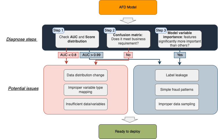
Check overall model performance: AUC and score distribution

More accurate prediction of future events is always the primary goal of a predictive model. The AUC returned by Amazon Fraud Detector is calculated on a properly sampled test set not used in training. In general, a model with an AUC greater than 0.9 is considered to be a good model.

If you observe a model with performance less than 0.8, it usually means the model has room for improvement (we discuss common issues for low model performance later in this post). Note that the definition of “good” performance highly depends on your business and the baseline model. You can still follow the steps in this post to improve your Amazon Fraud Detector model even though its AUC is greater than 0.8.

On the other hand, if the AUC is over 0.99, it means the model can almost perfectly separate the fraud and legitimate events on the test set. This is sometimes a “too good to be true” scenario (we discuss common issues for very high model performance later in this post).

Besides the overall AUC, the score distribution can also tell you how well the model is fitted. Ideally, you should see the bulk of legitimate and fraud located on the two ends of the scale, which indicates the model score can accurately rank the events on the test set.

In the following example, the score distribution has an AUC of 0.96.

If the legitimate and fraud distribution overlapped or concentrated in the center, it probably means the model doesn’t perform well on distinguishing fraud events from legitimate events, which might indicate historical data distribution changed or that you need more data or features.

The following is an example of score distribution with an AUC of 0.64.

If you can find a split point that can almost perfectly split fraud and legitimate events, there is a high chance that the model has a label leakage issue or the fraud patterns are too easy to detect, which should catch your attention.

In the following example, the score distribution has an AUC of 1.0.

Review business requirements: Confusion matrix and table

Although AUC is a convenient indicator of model performance, it may not directly translate to your business requirement. Amazon Fraud Detector also provides metrics such as fraud capture rate (true positive rate), percentage of legitimate events that are incorrectly predicted as fraud (false positive rate), and more, which are more commonly used as business requirements. After you train a model with a reasonably good AUC, you need to compare the model with your business requirement with those metrics.

The confusion matrix and table provide you with an interface to review the impact and check if it meets your business needs. Note that the numbers depend on the model threshold, where events with scores larger than then threshold are classified as fraud and events with scores lower than the threshold are classified as legit. You can choose which threshold to use depending on your business requirements.

For example, if your goal is to capture 73% of frauds, then (as shown in the example below) you can choose a threshold such as 855, which allows you to capture 73% of all fraud. However, the model will also mis-classify 3% legitimate events to be fraudulent. If this FPR is acceptable for your business, then the model is good for deployment. Otherwise, you need to improve the model performance.

Another example is if the cost for blocking or challenging a legitimate customer is extremely high, then you want a low FPR and high precision. In that case, you can choose a threshold of 950, as shown in the following example, which will miss-classify 1% of legitimate customers as fraud, and 80% of identified fraud will actually be fraudulent.

In addition, you can choose multiple thresholds and assign different outcomes, such as block, investigate, pass. If you can’t find proper thresholds and rules that satisfy all your business requirements, you should consider training your model with more data and attributes.

Check model variable importance

The Model variable importance pane displays how each variable contributes to your model. If one variable has a significantly higher importance value than the others, it might indicate label leakage or that the fraud patterns are too easy to detect. Note that the variable importance is aggregated back to your input variables. If you observe slightly higher importance of IP_ADDRESS, CARD_BIN, EMAIL_ADDRESS, PHONE_NUMBER, BILLING_ZIP, or SHIPPING_ZIP, it might because of the power of enrichment.

The following example shows model variable importance with a potential label leakage using investigation_status.

Model variable importance also gives you hints of what additional variables could potentially bring lift to the model. For example, if you observe low AUC and seller-related features show high importance, you might consider collecting more order features such as SELLER_CATEGORY, SELLER_ADDRESS, and SELLER_ACTIVE_YEARS, and add those variables to your model.

Common issues for low model performance

In this section, we discuss common issues you may encounter regarding low model performance.

Historical data distribution changed

Historical data distribution drift happens when you have a big business change or a data collection issue. For example, if you recently launched your product in a new market, the IP_ADDRESS, EMAIL, and ADDRESS related features could be completely different, and the fraud modus operandi could also change. Amazon Fraud Detector uses EVENT_TIMESTAMP to split data and evaluate your model on the appropriate subset of events in your dataset. If your historical data distribution changes significantly, the evaluation set could be very different from the training data, and the reported model performance could be low.

You can check the potential data distribution change issue by exploring your historical data:

  1. Use the Amazon Fraud Detector Data Profiler tool to check if the fraud rate and the missing rate of the label changed over time.
  2. Check if the variable distribution over time changed significantly, especially for features with high variable importance.
  3. Check the variable distribution over time by target variables. If you observe significantly more fraud events from one category in recent data, you might want to check if the change is reasonable using your business judgments.

If you find the missing rate of the label is very high or the fraud rate consistently dropped during the most recent dates, it might be an indicator of labels not fully matured. You should exclude the most recent data or wait longer to collect the accurate labels, and then retrain your model.

If you observe a sharp spike of fraud rate and variables on specific dates, you might want to double-check if it is an outlier or data collection issue. In that case, you should delete those events and retrain the model.

If you find the outdated data can’t represent your current and future business, you should exclude the old period of data from training. If you’re using stored events in Amazon Fraud Detector, you can simply retrain a new version and select the proper date range while configuring the training job. That may also indicate that the fraud modus operandi in your business changes relatively quickly over time. After model deployment, you may need to re-train your model frequently.

Improper variable type mapping

Amazon Fraud Detector enriches and transforms the data based on the variable types. It’s important that you map your variables to the correct type so that Amazon Fraud Detector model can take the maximum value of your data. For example, if you map IP to the CATEGORICAL type instead of IP_ADDRESS, you don’t get the IP-related enrichments in the backend.

In general, Amazon Fraud Detector suggests the following actions:

  1. Map your variables to specific types, such as IP_ADDRESS, EMAIL_ADDRESS, CARD_BIN, and PHONE_NUMBER, so that Amazon Fraud Detector can extract and enrich additional information.
  2. If you can’t find the specific variable type, map it to one of the three generic types: NUMERIC, CATEGORICAL, or FREE_FORM_TEXT.
  3. If a variable is in text form and has high cardinality, such as a customer review or product description, you should map it to the FREE_FORM_TEXT variable type so that Amazon Fraud Detector extracts text features and embeddings on the backend for you. For example, if you map url_string to FREE_FORM_TEXT, it’s able to tokenize the URL and extract information to feed into the downstream model, which will help it learn more hidden patterns from the URL.

If you find any of your variable types are mapped incorrectly in variable configuration, you can change your variable type and then retrain the model.

Insufficient data or features

Amazon Fraud Detector requires at least 10,000 records to train an Online Fraud Insights (OFI) or Transaction Fraud Insights (TFI) model, with at least 400 of those records identified as fraudulent. TFI also requires that both fraudulent records and legitimate records come from at least 100 different entities each to ensure the diversity of the dataset. Additionally, Amazon Fraud Detector requires the modeling data to have at least two variables. Those are the minimum data requirements to build a useful Amazon Fraud Detector model. However, using more records and variables usually helps the ML models better learn the underlying patterns from your data. When you observe a low AUC or can’t find thresholds that meet your business requirement, you should consider retraining your model with more data or add new features to your model. Usually, we find EMAIL_ADDRESS, IP, PAYMENT_TYPE, BILLING_ADDRESS, SHIPPING_ADDRESS, and DEVICE related variables are important in fraud detection.

Another possible cause is that some of your variables contain too many missing values. To see if that is happening, check the model training messages and refer to Troubleshoot training data issues for suggestions.

Common issues for very high model performance

In this section, we discuss common issues related to very high model performance.

Label leakage

Label leakage occurs when the training datasets use information that would not be expected to be available at prediction time. It overestimates the model’s utility when run in a production environment.

High AUC (close to 1), perfectly separated score distribution, and significantly higher variable importance of one variable could be indicators of potential label leakage issues. You can also check the correlation between the features and the label using the Data Profiler. The Feature and label correlation plot shows the correlation between each feature and the label. If one feature has over 0.99 correlation with the label, you should check if the feature is used properly based on business judgments. For example, to build a risk model to approve or decline a loan application, you shouldn’t use the features like AMOUNT_PAID, because the payments happen after the underwriting process. If a variable isn’t available at the time you make prediction, you should remove that variable from model configuration and retrain a new model.

The following example shows the correlation between each variable and label. investigation_status has a high correlation (close to 1) with the label, so you should double-check if there is a label leakage issue.

Simple fraud patterns

When the fraud patterns in your data are simple, you might also observe very high model performance. For example, suppose all the fraud events in the modeling data come through the same Internal Service Provider; it’s straightforward for the model to pick the IP-related variables and return a “perfect” model with high importance of IP.

Simple fraud patterns don’t always indicate a data issue. It could be true that the fraud modus operandi in your business is easy to capture. However, before making a conclusion, you need to make sure the labels used in model training are accurate, and the modeling data covers as many fraud patterns as possible. For example, if you label your fraud events based on rules, such as labeling all applications from a specific BILLING_ZIP plus PRODUCT_CATEGORY as fraud, the model can easily catch those frauds by simulating the rules and achieving a high AUC.

You can check the label distribution across different categories or bins of each feature using the Data Profiler. For example, if you observe that most fraud events come from one or a few product categories, it might be an indicator of simple fraud patterns, and you need to confirm that it’s not a data collection or process mistake. If the feature is like CUSTOMER_ID, you should exclude the feature in model training.

The following example shows label distribution across different categories of product_category. All fraud comes from two product categories.

Improper data sampling

Improper data sampling may happen when you sampled and only sent part of your data to Amazon Fraud Detector. If the data isn’t sampled properly and isn’t representative of the traffic in production, the reported model performance will be inaccurate and the model could be useless for production prediction. For example, if all fraud events in the modeling data are sampled from Asia and all legit events are sampled from the US, the model might learn to separate fraud and legit based on BILLING_COUNTRY. In that case, the model is not generic to be applied to other populations.

Usually, we suggest sending all the latest events without sampling. Based on the data size and fraud rate, Amazon Fraud Detector does sampling before model training for you. If your data is too large (over 100 GB) and you decide to sample and send only a subset, you should randomly sample your data and make sure the sample is representative of the entire population. For TFI, you should sample your data by entity, which means if one entity is sampled, you should include all its history so that the entity level aggregates are calculated correctly. Note that if you only send a subset of data to Amazon Fraud Detector, the real-time aggregates during inference might be inaccurate if the previous events of the entities aren’t sent.

Another improper data sampling could be only using a short period of data, like one day’s data, to build the model. The data might be biased, especially if your business or fraud attacks have seasonality. We usually recommend including at least two cycles’ (such as 2 weeks or 2 months) worth of data in the modeling to ensure the diversity of fraud types.

Conclusion

After diagnosing and resolving all the potential issues, you should get a useful Amazon Fraud Detector model and be confident about its performance. For the next step, you can create a detector with the model and your business rules, and be ready to deploy it to production for a shadow mode evaluation.

Appendix

How to exclude variables for model training

After the deep dive, you might identify a variable leak target information, and want to exclude it from model training. You can retrain a model version excluding the variables you don’t want by completing the following steps:

  1. On the Amazon Fraud Detector console, in the navigation pane, choose Models.
  2. On the Models page, choose the model you want to retrain.
  3. On the Actions menu, choose Train new version.
  4. Select the date range you want to use and choose Next.
  5. On the Configure training page, deselect the variable you don’t want to use in model training.
  6. Specify your fraud labels and legitimate labels and how you want Amazon Fraud Detector to use unlabeled events, then choose Next.
  7. Review the model configuration and choose Create and train model.

How to change event variable type

Variables represent data elements used in fraud prevention. In Amazon Fraud Detector, all variables are global and are shared across all events and models, which means one variable could be used in multiple events. For example, IP could be associated with sign-in events, and it could also be associated with transaction events. Naturally, Amazon Fraud Detector locked the variable type and data type once a variable is created. To delete an existing variable, you need to first delete all associated event types and models. You can check the resources associated with the specific variable by navigating to Amazon Fraud Detector, choosing Variables in the navigation pane, and choosing the variable name and Associated resources.

Delete the variable and all associated event types

To delete the variable, complete the following steps:

  1. On the Amazon Fraud Detector console, in the navigation pane, choose Variables.
  2. Choose the variable you want to delete.
  3. Choose Associated resources to view a list of all the event types used this variable.
    You need to delete those associated event types before deleting the variable.
  4. Choose the event types in the list to go to the associated event type page.
  5. Choose Stored events to check if any data is stored under this event type.
  6. If there are events stored in Amazon Fraud Detector, choose Delete stored events to delete the stored events.
    When the delete job is complete, the message “The stored events for this event type were successfully deleted” appears.
  7. Choose Associated resources.
    If detectors and models are associated with this event type, you need to delete those resources first.
  8. If detectors are associated, complete the following steps to delete all associated detectors:
    1. Choose the detector to go to the Detector details page.
    2. In the Model versions pane, choose the detector’s version.
    3. On the detector version page, choose Actions.
    4. If the detector version is active, choose Deactivate, choose Deactivate this detector version without replacing it with a different version, and choose Deactivate detector version.
    5. After the detector version is deactivated, choose Actions and then Delete.
    6. Repeat these steps to delete all detector versions.
    7. On the Detector details page, choose Associated rules.
    8. Choose the rule to delete.
    9. Choose Actions and Delete rule version.
    10. Enter the rule name to confirm and choose Delete version.
    11. Repeat these steps to delete all associated rules.
    12. After all detector versions and associated rules are deleted, go to the Detector details page, choose Actions, and choose Delete detector.
    13. Enter the detector’s name and choose Delete detector.
    14. Repeat these steps to delete the next detector.
  9. If any models are associated with the event type, complete the following steps to delete them:
    1. Choose the name of the model.
    2. In the Model versions pane, choose the version.
    3. If the model status is Active, choose Actions and Undeploy model version.
    4. Enter undeploy to confirm and choose Undeploy model version.
      The status changes to Undeploying. The process takes a few minutes to complete.
    5. After the status becomes Ready to deploy, choose Actions and Delete.
    6. Repeat these steps to delete all model versions.
    7. On the Model details page, choose Actions and Delete model.
    8. Enter the name of the model and choose Delete model.
    9. Repeat these steps to delete the next model.
  10. After all associated detectors and models are deleted, choose Actions and Delete event type on the Event details page.
  11. Enter the name of the event type and choose Delete event type.
  12. In the navigation pane, choose Variables, and choose the variable you want to delete.
  13. Repeat the earlier steps to delete all event types associated with the variable.
  14. On the Variable details page, choose Actions and Delete.
  15. Enter the name of the variable and choose Delete variable.

Create a new variable with the correct variable type

After you have deleted the variable and all associated event types, stored events, models, and detectors from Amazon Fraud Detector, you can create a new variable of the same name and map it to the correct variable type.

  1. On the Amazon Fraud Detector console, in the navigation pane, choose Variables.
  2. Choose Create.
  3. Enter the variable name you want to modify (the one you deleted earlier).
  4. Select the correct variable type you want to change to.
  5. Choose Create variable.

Upload data and retrain the model

After you update the variable type, you can upload the data again and train a new model. For instructions, refer to Detect online transaction fraud with new Amazon Fraud Detector features.

How to add new variables to an existing event type

To add new variables to the existing event type, complete the following steps:

  1. Add the new variables to the previous training CVS file.
  2. Upload the new training data file to an S3 bucket. Note the Amazon S3 location of your training file (for example, s3://bucketname/path/to/some/object.csv) and your role name.
  3. On the Amazon Fraud Detector console, in the navigation pane, choose Events.
  4. On the Event types page, choose the name of the event type you want to add variables.
  5. On the Event type details page, choose Actions, then Add variables.
  6. Under Choose how to define this event’s variables, choose Select variables from a training dataset.
  7. For IAM role, select an existing IAM role or create a new role to access data in Amazon S3.
  8. For Data location, enter the S3 location of the new training file and choose Upload.
    The new variables not present in the existing event type should show up in the list.
  9. Choose Add variables.

Now, the new variables have been added to the existing event type. If you’re using stored events in Amazon Fraud Detector, the new variables of the stored events are still missing. You need to import the training data with the new variables to Amazon Fraud Detector and then retrain a new model version. When uploading the new training data with the same EVENT_ID and EVENT_TIMESTAMP, the new event variables overwrite the previous event variables stored in Amazon Fraud Detector.


About the Authors

Julia Xu is a Research Scientist with Amazon Fraud Detector. She is passionate about solving customer challenges using Machine Learning techniques. In her free time, she enjoys hiking, painting, and exploring new coffee shops.

Hao Zhou is a Research Scientist with Amazon Fraud Detector. He holds a PhD in electrical engineering from Northwestern University, USA. He is passionate about applying machine learning techniques to combat fraud and abuse.

Abhishek Ravi is a Senior Product Manager with Amazon Fraud Detector. He is passionate about leveraging technical capabilities to build products that delight customers.

Read More

Reducing gender-based harms in AI with Sunipa Dev

Natural language processing (NLP) is a form of artificial intelligence that teaches computer programs how to take in, interpret, and produce language from large data sets. For example, grammar checkers use NLP to come up with grammar suggestions that help people write grammatically correct phrases. But as Google’s AI Principles note, it’s sometimes necessary to have human intervention to identify risks of unfair bias.

Sunipa Dev is a research scientist at Google who focuses on Responsible AI. Some of her work focuses specifically on ways to evaluate unfair bias in NLP outcomes, reducing harms for people with queer and non-binary identities. Sunipa’s work was recently featured at a workshop at the ACM Fairness, Accountability, and Transparency (FAcct) conference in Seoul, Korea.

In our interview, she emphasizes that her work is achievable only through forging collaborative partnerships between researchers, engineers, and AI practitioners with everyday users and communities.

What inspired you to take on this career path?

While working on my PhD at the University of Utah, I explored research questions such as, “How do we evaluate NLP tech if they contain biases?” As language models evolved, our questions about potential harms did, too. During my postdoc work at UCLA, we ran a study to evaluate challenges in various language models by surveying respondents who identified as non-binary and had some experience with AI. With a focus on gender bias, our respondents helped us understand that experiences with language technologies cannot be understood in isolation. Rather, we must consider how these technologies intersect with systemic discrimination, erasure, and marginalization. For example, the harm of misgendering by a language technology can be compounded for trans, non-binary, and gender-diverse individuals who are already fighting against society to defend their identities. And when it’s in your personal space, like on your devices while emailing or texting, these small jabs can build up to larger psychological damage.

What is your current role at Google?

I am currently a Research Scientist at the Responsible AI – Human Centered Technology team. In my current role, I am working to build a better understanding of how to avoid unfair bias in AI language models across different cultures and geographies, aligned with Google’s AI Principles.

This is a challenge because language changes, and so do cultures and regional laws as we move from one place to another. This can all impact how people express themselves, what identities they choose and how they experience discrimination on a daily basis. Gender bias can manifest in entirely different ways in different parts of the world. In some of my ongoing work that focuses on a non-Western point of view, we are working with social scientists and NGOs in India while engaging with local communities. We are using the voices of many people who are living in a specific region and asking, “What are the biases prevalent in their society?”

What is gender bias in NLP?

Written text and training data for language technologies can lack representation or misrepresent different gender identities; this can reflect social biases. As a result, some NLP technologies can reinforce gender stereotypes and slurs, erase people’s gender identities, or have reduced quality of service for marginalized communities. What drives me in my work is my goal to make language technologies more inclusive and usable.

Why does this matter for AI?

Gender can be such an integral part of someone’s identity, and having that wrongly assumed by an AI system can be triggering, unfair, and harmful. We need to work towards systems and societies that do not encode unfair biases and harmful stereotypes in order to break out of the cycle of perpetuating harms of stereotyping, misgendering, and erasure.

How can people who are not researchers, engineers or AI practitioners engage in this work?

A very direct way is for people to report potential harms as bugs within products they use. People can also participate in open discussions in workshops, panels and town halls. These are all helpful ways to build inclusive AI.

I want to emphasize, however, that the onus can’t only be on the user. It’s also on the side of the researcher, engineer and AI practitioner. The goal is to create a continuous feedback loop between humans and machines, with real people stepping in to ensure the creation of more responsible AI. As AI practitioners, we need to work with the people we’re trying to serve and have users collaborate with us to tell us what we need to do better.

Read More