Addressing and mitigating the effects of climate change requires a collective effort, bringing our strengths to bear across industry, government, academia, and civil society. As we continue to explore the role of technology to advance the art of the possible, we are launching the Microsoft Climate Research Initiative (MCRI). This community of multi-disciplinary researchers is working together to accelerate cutting-edge research and transformative innovation in climate science and technology.
MCRI enables us to bring Microsoft’s research skills and compute capacities to deep and continuous collaboration with domain experts. For the kickoff of this initiative, we are focusing on three critical areas in climate research where computational advances can drive key scientific transformations: Overcoming constraints to decarbonization, reducing uncertainties in carbon accounting, and assessing climate risks in more detail.
Through these collaborative research projects, we hope to develop and sustain a highly engaged research ecosystem comprising a diversity of perspectives. Researchers will offer transdisciplinary and diverse expertise, particularly in areas beyond traditional computer science, such as environmental science, chemistry, and a variety of engineering disciplines. All results of this initiative are expected to be made public and freely available to spark even broader research and progress on these important climate issues.
“As researchers, we’re excited to work together on projects specifically selected for their potential impact on global climate challenges. With Microsoft’s computational capabilities and the domain expertise from our collaborators, our complementary strengths can accelerate progress in incredible ways.”
– Karin Strauss, Microsoft
Microsoft researchers will be working with collaborators globally to co-investigate priority climate-related topics and bring innovative, world-class research to influential journals and venues.
Phase one collaborations
Carbon accounting
Real-time Monitoring of Carbon Control Progress from CO2 and Air Pollutant Observations with a Physically informed Transformer-based Neural Network
Understanding the change in CO2 emissions from the measurement of CO2 concentrations such as that done by satellites is very useful in tracking the real-time progress of carbon reduction actions. Current CO2 observations are relatively limited: numerical model-based methods have very low calculation efficiency. The proposed study aims to develop a novel method that combines atmospheric numerical modeling and machine learning to infer the CO2 emissions from satellite observations and ground monitor sensor data.
AI based Near-real-time Global Carbon Budget (ANGCB)
Zhu Liu, Tsinghua University; Biqing Zhu and Philippe Ciais, LSCE; Steven J. Davis, UC Irvine; Wei Cao, and Jiang Bian , Microsoft
Mitigation of climate change will depend upon a carbon emission trajectory that successfully achieves carbon neutrality by 2050. To that end, a global carbon budget assessment is essential. The AI-based, near-real-time Global Carbon Budget (ANGCB) project aims to provide the world’s first global carbon budget assessment based on Artificial Intelligence (AI) and other data science technologies.
Carbon reduction and removal
Computational Discovery of Novel Metal–Organic Frameworks for Carbon Capture
Removing CO2 from the environment is expected to be an integral component of keeping temperature rise below 1.5°C. However, today this is an inefficient and expensive undertaking. This project will apply generative machine learning to the design of new metal–organic frameworks (MOFs) to optimize for low-cost removal of CO2 from air and other dilute gas streams.
An Assessment of Liquid Metal Catalyzed CO2 Reduction
The CO2 reduction process can be used to convert captured carbon into a storable form as well as to manufacture sustainable fuels and materials with lower environmental impacts. This project will evaluate liquid metal-based reduction processes, identifying advantages, pinch-points, and opportunities for improvement needed to reach industrial-relevant scales. It will lay the foundation for improving catalysts and address scaling bottlenecks.
Computational Design and Characterization of Organic Electrolytes for Flow Battery and Carbon Capture Applications
Energy storage is essential to enable 100% zero-carbon electricity generation. This work will use generative machine learning models and quantum mechanical modeling to drive the discovery and optimization of a new class of organic molecules for energy-efficient electrochemical energy storage and carbon capture.
Despite encouraging progress in recycling, many plastic polymers often end up being one-time-use materials. The plastics that compose printed circuit boards (PCBs), ubiquitous in every modern device, are amongst those most difficult to recycle. Vitrimers, a new class of polymers that can be recycled multiple times without significant changes in material properties, present a promising alternative. This project will leverage advances in machine learning to select vitrimer formulations that withstand the requirements imposed by their use in PCBs.
The concrete industry is a major contributor to greenhouse gas emissions, the majority of which can be attributed to cement. The discovery of alternative cements is a promising avenue for decreasing the environmental impacts of the industry. This project will employ machine learning methods to accelerate mechanical property optimization of “green” cements that meet application quality constraints while minimizing carbon footprint.
Environmental resilience
Causal Inference to Understand the Impact of Humanitarian Interventions on Food Security in Africa
The Causal4Africa project will investigate the problem of food security in Africa from a novel causal inference standpoint. The project will illustrate the usefulness of causal discovery and estimation of effects from observational data by intervention analysis. Ambitiously, it will improve the usefulness of causal ML approaches for climate risk assessment by enabling the interpretation and evaluation of the likelihood and potential consequences of specific interventions.
Improving Subseasonal Forecasting with Machine Learning
Water and fire managers rely on subseasonal forecasts two to six weeks in advance to allocate water, manage wildfires, and prepare for droughts and other weather extremes. However, skillful forecasts for the subseasonal regime are lacking due to a complex dependence on local weather, global climate variables, and the chaotic nature of weather. To address this need, this project will use machine learning to adaptively correct the biases in traditional physics-based forecasts and adaptively combine the forecasts of disparate models.
Editor’s note: This post is part of our weekly In the NVIDIA Studio series, which celebrates featured artists, offers creative tips and tricks, and demonstrates how NVIDIA Studio technology accelerates creative workflows.
The June NVIDIA Studio Driver is available for download today, optimizing the latest creative app updates, all with the stability and reliability that users count on.
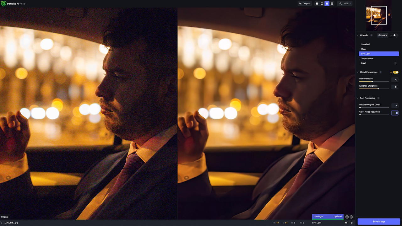
Creators with NVIDIA RTX GPUs will benefit from faster performance and new features within Blender version 3.2, BorisFX Sapphire release 2022.5 and Topaz Denoise AI 3.7.0.
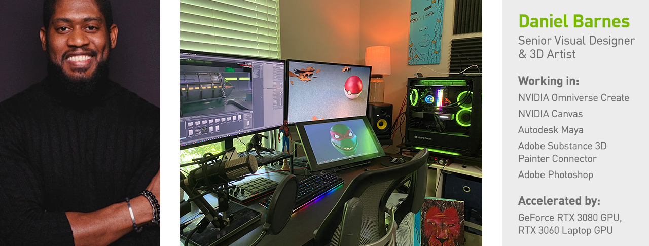
And this week, NVIDIA Senior Designer Daniel Barnes showcases inspirational artwork In the NVIDIA Studio. Specializing in visual design and 3D content, Barnes covers his creative workflow in designing the galactic 3D scene Journey.
June Boon: Studio Driver Release Supports Blender, Sapphire and Denoise AI Updates
OpenVDB offers a near-infinite 3D index space, allowing massive Universal Scene Description (USD) files to move in and out of Omniverse while keeping these volumes intact. 3D artists can iterate with larger files, speeding up creative workflows without the need to reduce or convert files and sizes.
Light sources from the interior, pool, benches and greater world combine for a breathtaking visual built in the Blender compositor without added re-render work.
Blender 3.2 also added a Light Group feature, enabling artists to modify the color and intensity of light sources in the compositor without re-rendering. New Shadow Caustics supports selective rendering of caustics in shadows of refractive objects for further realism. Check out a complete overview of the Blender 3.2 update.
BorisFX Sapphire 2022.5 now supports multi-GPU systems applying GPU-accelerated visual-effect plugins in Blackmagic’s DaVinci Resolve — scaling GPU power with rendering speeds up to 6x faster.
Topaz Denoise AI accelerated by the NVIDIA TensorRT framework provides more consistent color while reducing blotchiness in highlights and shadows.
Topaz Denoise AI 3.7.0 added support for the NVIDIA TensorRT framework, which means RTX GPU owners will benefit from significantly faster inference speeds. When using RAW model denoising features, inference runs up to 6x faster.
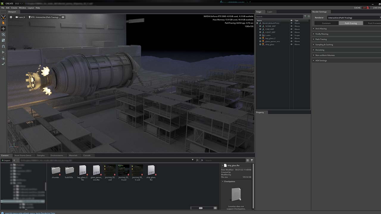
This week’s In the NVIDIA Studio artist spotlight sees NVIDIA’s Daniel Barnes share his creative process for the 3D sci-fi scene, Journey.
Barnes’ artwork draws inspiration from various movies and anime, usually a combination of visual revelations. Journey is an extension of Barnes’ latest obsession, the isekai genre in anime, where the protagonist awakens in another world and has to navigate their new and unknown situation.
“This reincarnation narrative can be pretty refreshing, as it almost always is something you can connect with living life and having firsts, or wishing you could redo a particular moment differently with the advantage of 20/20 hindsight,” Barnes noted.
Barnes first visualized ‘Journey’ in Adobe Photoshop.
Barnes sketches when inspiration strikes — often at his local coffee shop — which is where he got started with Journey using Adobe Photoshop.
With his GeForce RTX 3060-powered laptop, Barnes benefited from speedy GPU-accelerated features such as Scrubby Zoom, to quickly zoom and adjust fine details, and Flick Panning, to move around the canvas faster, with the freedom to create on the go.
Turning his attention to Autodesk Maya, Barnes built and blocked out foundational geometric shapes for the Journey scene, starting with elements he could reuse from an existing scene. “Absolutely nothing wrong with working smart wherever possible,” Barnes mused. The GPU-accelerated viewport unlocks fast and interactive 3D modeling for Barnes, who was able to set up the building blocks quickly.
Barnes further detailed some 3D models in ZBrush by sculpting with custom brushes. He then ran the ZBrush Remesh feature, creating a new single mesh by combining several existing objects. This simplified applying textures and will make potentially animating Journey much easier.
Omniverse Create’s material presets and lighting allowed Barnes to work faster and more efficiently.
Barnes then used the Omniverse Create app to assemble his physically accurate, photorealistic 3D scene. Back at home with his RTX 3080-powered desktop system, he used the built-in RTX Renderer for interactive visualization within the viewport with virtually no slowdown. Even building at real-world scale, Create’s material presets and lighting allowed Barnes to quickly and efficiently apply realistic visuals with ease.
Barnes bounced back and forth between the handy Adobe Substance 3D Painter Connector and the Omniverse NVIDIA vMaterials library to discover, create and refine textures, applying his unique color scheme style in Create.
AI in the Studio suite of apps, Omniverse Create and NVIDIA Canvas played key roles in developing ‘Journey.’
With the piece in good shape, Barnes planned for the composite by exporting several versions with depth of field, extra light bloom and fog enabled.
Now, all Journey needed was a vibrant sky to complete the piece. Barnes harnessed the power of AI with the NVIDIA Canvas app, free for RTX GPU owners, turning simple brushstrokes into a realistic, stunning view. Barnes generated outer space in mere minutes, allowing for more concept exploration and saving the time required to search for backgrounds or create one from scratch.
The artist then returned to Adobe Photoshop to add color bleed and stylish details, drop in the Canvas background, and export final renders.
NVIDIA Senior Visual Designer and 3D artist Daniel Barnes.
Check out Barnes’ Instagram for more design inspiration.
Members of the public sector, private sector, and academia convened for the second AI Policy Forum Symposium last month to explore critical directions and questions posed by artificial intelligence in our economies and societies.
The virtual event, hosted by the AI Policy Forum (AIPF) — an undertaking by the MIT Schwarzman College of Computing to bridge high-level principles of AI policy with the practices and trade-offs of governing — brought together an array of distinguished panelists to delve into four cross-cutting topics: law, auditing, health care, and mobility.
In the last year there have been substantial changes in the regulatory and policy landscape around AI in several countries — most notably in Europe with the development of the European Union Artificial Intelligence Act, the first attempt by a major regulator to propose a law on artificial intelligence. In the United States, the National AI Initiative Act of 2020, which became law in January 2021, is providing a coordinated program across federal government to accelerate AI research and application for economic prosperity and security gains. Finally, China recently advanced several new regulations of its own.
Each of these developments represents a different approach to legislating AI, but what makes a good AI law? And when should AI legislation be based on binding rules with penalties versus establishing voluntary guidelines?
Jonathan Zittrain, professor of international law at Harvard Law School and director of the Berkman Klein Center for Internet and Society, says the self-regulatory approach taken during the expansion of the internet had its limitations with companies struggling to balance their interests with those of their industry and the public.
“One lesson might be that actually having representative government take an active role early on is a good idea,” he says. “It’s just that they’re challenged by the fact that there appears to be two phases in this environment of regulation. One, too early to tell, and two, too late to do anything about it. In AI I think a lot of people would say we’re still in the ‘too early to tell’ stage but given that there’s no middle zone before it’s too late, it might still call for some regulation.”
A theme that came up repeatedly throughout the first panel on AI laws — a conversation moderated by Dan Huttenlocher, dean of the MIT Schwarzman College of Computing and chair of the AI Policy Forum — was the notion of trust. “If you told me the truth consistently, I would say you are an honest person. If AI could provide something similar, something that I can say is consistent and is the same, then I would say it’s trusted AI,” says Bitange Ndemo, professor of entrepreneurship at the University of Nairobi and the former permanent secretary of Kenya’s Ministry of Information and Communication.
Eva Kaili, vice president of the European Parliament, adds that “In Europe, whenever you use something, like any medication, you know that it has been checked. You know you can trust it. You know the controls are there. We have to achieve the same with AI.” Kalli further stresses that building trust in AI systems will not only lead to people using more applications in a safe manner, but that AI itself will reap benefits as greater amounts of data will be generated as a result.
The rapidly increasing applicability of AI across fields has prompted the need to address both the opportunities and challenges of emerging technologies and the impact they have on social and ethical issues such as privacy, fairness, bias, transparency, and accountability. In health care, for example, new techniques in machine learning have shown enormous promise for improving quality and efficiency, but questions of equity, data access and privacy, safety and reliability, and immunology and global health surveillance remain at large.
MIT’s Marzyeh Ghassemi, an assistant professor in the Department of Electrical Engineering and Computer Science and the Institute for Medical Engineering and Science, and David Sontag, an associate professor of electrical engineering and computer science, collaborated with Ziad Obermeyer, an associate professor of health policy and management at the University of California Berkeley School of Public Health, to organize AIPF Health Wide Reach, a series of sessions to discuss issues of data sharing and privacy in clinical AI. The organizers assembled experts devoted to AI, policy, and health from around the world with the goal of understanding what can be done to decrease barriers to access to high-quality health data to advance more innovative, robust, and inclusive research results while being respectful of patient privacy.
Over the course of the series, members of the group presented on a topic of expertise and were tasked with proposing concrete policy approaches to the challenge discussed. Drawing on these wide-ranging conversations, participants unveiled their findings during the symposium, covering nonprofit and government success stories and limited access models; upside demonstrations; legal frameworks, regulation, and funding; technical approaches to privacy; and infrastructure and data sharing. The group then discussed some of their recommendations that are summarized in a report that will be released soon.
One of the findings calls for the need to make more data available for research use. Recommendations that stem from this finding include updating regulations to promote data sharing to enable easier access to safe harbors such as the Health Insurance Portability and Accountability Act (HIPAA) has for de-identification, as well as expanding funding for private health institutions to curate datasets, amongst others. Another finding, to remove barriers to data for researchers, supports a recommendation to decrease obstacles to research and development on federally created health data. “If this is data that should be accessible because it’s funded by some federal entity, we should easily establish the steps that are going to be part of gaining access to that so that it’s a more inclusive and equitable set of research opportunities for all,” says Ghassemi. The group also recommends taking a careful look at the ethical principles that govern data sharing. While there are already many principles proposed around this, Ghassemi says that “obviously you can’t satisfy all levers or buttons at once, but we think that this is a trade-off that’s very important to think through intelligently.”
In addition to law and health care, other facets of AI policy explored during the event included auditing and monitoring AI systems at scale, and the role AI plays in mobility and the range of technical, business, and policy challenges for autonomous vehicles in particular.
The AI Policy Forum Symposium was an effort to bring together communities of practice with the shared aim of designing the next chapter of AI. In his closing remarks, Aleksander Madry, the Cadence Designs Systems Professor of Computing at MIT and faculty co-lead of the AI Policy Forum, emphasized the importance of collaboration and the need for different communities to communicate with each other in order to truly make an impact in the AI policy space.
“The dream here is that we all can meet together — researchers, industry, policymakers, and other stakeholders — and really talk to each other, understand each other’s concerns, and think together about solutions,” Madry said. “This is the mission of the AI Policy Forum and this is what we want to enable.”
Amazon Polly is a leading cloud-based service that converts text into lifelike speech. Following the adoption of Neural Text-to-Speech (NTTS), we have continuously expanded our portfolio of available voices in order to provide a wide selection of distinct speakers in supported languages. Today, we are pleased to announce four new additions: Pedro speaking US Spanish, Daniel speaking German, Liam speaking Canadian French, and Arthur speaking British English. As with all the Neural voices in our portfolio, these voices offer fluent, native pronunciation in their target languages. However, what is unique about these four voices is that they are all based on the same voice persona.
Pedro, Daniel, Liam and Arthur were modeled on an existing US English Matthew voice. While customers continue to appreciate Matthew for his naturalness and professional-sounding quality, the voice has so far exclusively served English-speaking traffic. Now, using deep-learning methods, we decoupled language and speaker identity, which allowed us to preserve native-like fluency across many languages without having to obtain multilingual data from the same speaker. In practice, this means that we transferred the vocal characteristics of the US English Matthew voice to US Spanish, German, Canadian French, and British English, opening up new opportunities for Amazon Polly customers.
Having a similar-sounding voice available in five locales unlocks great potential for business growth. First of all, customers with a global footprint can create a consistent user experience across languages and regions. For example, an interactive voice response (IVR) system that supports multiple languages can now serve different customer segments without changing the feel of the brand. The same goes for all other TTS use cases, such as voicing news articles, education materials, or podcasts.
Secondly, the voices are a good fit for Amazon Polly customers who are looking for a native pronunciation of foreign phrases in any of the five supported languages.
Thirdly, releasing Pedro, Daniel, Liam, and Arthur serves our customers who like Amazon Polly NTTS in US Spanish, German, Canadian French, and British English but are looking for a high-quality masculine voice—they can use these voices to create audio for monolingual content and expect top quality that is on par with other NTTS voices in these languages.
Lastly, the technology we have developed to create the new male NTTS voices can also be used for Brand Voices. Thanks to this, Brand Voice customers can not only enjoy a unique NTTS voice that is tailored to their brand, but also keep a consistent experience while serving an international audience.
Example use case
Let’s explore an example use case to demonstrate what this means in practice. Amazon Polly customers familiar with Matthew can still use this voice in the usual way by choosing Matthew on the Amazon Polly console and entering any text they want to hear spoken in US English. In the following scenario, we generate audio samples for an IVR system (“For English, please press one”):
Thanks to this release, you can now expand the use case to deliver a consistent audio experience in different languages. All the new voices are natural-sounding and maintain a native-like accent.
To generate speech in British English, choose Arthur (“For English, please press one”):
To use a US Spanish speaker, choose Pedro (“Para español, por favor marque dos”):
Daniel offers support in German (“Für Deutsch drücken Sie bitte die Drei”):
You can synthesize text in Canadian French by choosing Liam (“Pour le français, veuillez appuyer sur le quatre”):
Note that apart from speaking with a different accent, the UK English Arthur voice will localize the input text differently than the US English Matthew voice. For example, “1/2/22” will be read by Arthur as “the 1st of February 2022,” whereas Matthew will read it as “January 2nd 2022.”
Now let’s combine these prompts:
Conclusion
Pedro, Daniel, Liam, and Arthur are available as Neural TTS voices only, so in order to enjoy them, you need to use the Neural engine in one of the AWS Regions supporting NTTS. These are high-quality monolingual voices in their target languages. The fact that their personas are consistent across languages is an additional benefit, which we hope will delight customers working with content in multiple languages. For more details, review our full list of Amazon Polly text-to-speech voices , Neural TTS pricing, service limits, and FAQs, and visit our pricing page.
About the Authors
Patryk Wainaina is a Language Engineer working on text-to-speech for English, German, and Spanish. With a background in speech and language processing, his interests lie in machine learning as applied to TTS front-end solutions, particularly in low-resource settings. In his free time, he enjoys listening to electronic music and learning new languages.
Marta Smolarek is a Senior Program Manager in the Amazon Text-to-Speech team, where she is focused on the Contact Center TTS use case. She defines Go-to-Market initiatives, uses customer feedback to build the product roadmap and coordinates TTS voice launches. Outside of work, she loves to go camping with her family.
Amazon SageMaker provides a suite of built-in algorithms, pre-trained models, and pre-built solution templates to help data scientists and machine learning (ML) practitioners get started on training and deploying ML models quickly. You can use these algorithms and models for both supervised and unsupervised learning. They can process various types of input data, including tabular, image, and text.
Starting today, SageMaker provides four new built-in tabular data modeling algorithms: LightGBM, CatBoost, AutoGluon-Tabular, and TabTransformer. You can use these popular, state-of-the-art algorithms for both tabular classification and regression tasks. They’re available through the built-in algorithms on the SageMaker console as well as through the Amazon SageMaker JumpStart UI inside Amazon SageMaker Studio.
The following is the list of the four new built-in algorithms, with links to their documentation, example notebooks, and source.
In the following sections, we provide a brief technical description of each algorithm, and examples of how to train a model via the SageMaker SDK or SageMaker Jumpstart.
LightGBM
LightGBM is a popular and efficient open-source implementation of the Gradient Boosting Decision Tree (GBDT) algorithm. GBDT is a supervised learning algorithm that attempts to accurately predict a target variable by combining an ensemble of estimates from a set of simpler and weaker models. LightGBM uses additional techniques to significantly improve the efficiency and scalability of conventional GBDT.
CatBoost
CatBoost is a popular and high-performance open-source implementation of the GBDT algorithm. Two critical algorithmic advances are introduced in CatBoost: the implementation of ordered boosting, a permutation-driven alternative to the classic algorithm, and an innovative algorithm for processing categorical features. Both techniques were created to fight a prediction shift caused by a special kind of target leakage present in all currently existing implementations of gradient boosting algorithms.
AutoGluon-Tabular
AutoGluon-Tabular is an open-source AutoML project developed and maintained by Amazon that performs advanced data processing, deep learning, and multi-layer stack ensembling. It automatically recognizes the data type in each column for robust data preprocessing, including special handling of text fields. AutoGluon fits various models ranging from off-the-shelf boosted trees to customized neural network models. These models are ensembled in a novel way: models are stacked in multiple layers and trained in a layer-wise manner that guarantees raw data can be translated into high-quality predictions within a given time constraint. Over-fitting is mitigated throughout this process by splitting the data in various ways with careful tracking of out-of-fold examples. AutoGluon is optimized for performance, and its out-of-the-box usage has achieved several top-3 and top-10 positions in data science competitions.
TabTransformer
TabTransformer is a novel deep tabular data modelling architecture for supervised learning. The TabTransformer is built upon self-attention based Transformers. The Transformer layers transform the embeddings of categorical features into robust contextual embeddings to achieve higher prediction accuracy. Furthermore, the contextual embeddings learned from TabTransformer are highly robust against both missing and noisy data features, and provide better interpretability. This model is the product of recent Amazon Science research (paper and official blog post here) and has been widely adopted by the ML community, with various third-party implementations (Keras, AutoGluon,) and social media features such as tweets, towardsdatascience, medium, and Kaggle.
Benefits of SageMaker built-in algorithms
When selecting an algorithm for your particular type of problem and data, using a SageMaker built-in algorithm is the easiest option, because doing so comes with the following major benefits:
The built-in algorithms require no coding to start running experiments. The only inputs you need to provide are the data, hyperparameters, and compute resources. This allows you to run experiments more quickly, with less overhead for tracking results and code changes.
The built-in algorithms come with parallelization across multiple compute instances and GPU support right out of the box for all applicable algorithms (some algorithms may not be included due to inherent limitations). If you have a lot of data with which to train your model, most built-in algorithms can easily scale to meet the demand. Even if you already have a pre-trained model, it may still be easier to use its corollary in SageMaker and input the hyperparameters you already know rather than port it over and write a training script yourself.
You are the owner of the resulting model artifacts. You can take that model and deploy it on SageMaker for several different inference patterns (check out all the available deployment types) and easy endpoint scaling and management, or you can deploy it wherever else you need it.
Let’s now see how to train one of these built-in algorithms.
Train a built-in algorithm using the SageMaker SDK
To train a selected model, we need to get that model’s URI, as well as that of the training script and the container image used for training. Thankfully, these three inputs depend solely on the model name, version (for a list of the available models, see JumpStart Available Model Table), and the type of instance you want to train on. This is demonstrated in the following code snippet:
from sagemaker import image_uris, model_uris, script_uris

train_model_id, train_model_version, train_scope = "lightgbm-classification-model", "*", "training"
training_instance_type = "ml.m5.xlarge"

# Retrieve the docker image
train_image_uri = image_uris.retrieve(
    region=None,
    framework=None,
    model_id=train_model_id,
    model_version=train_model_version,
    image_scope=train_scope,
    instance_type=training_instance_type
)
# Retrieve the training script
train_source_uri = script_uris.retrieve(
    model_id=train_model_id, model_version=train_model_version, script_scope=train_scope
)
# Retrieve the model artifact; in the tabular case, the model is not pre-trained
train_model_uri = model_uris.retrieve(
    model_id=train_model_id, model_version=train_model_version, model_scope=train_scope
)
The train_model_id changes to lightgbm-regression-model if we’re dealing with a regression problem. The IDs for all the other models introduced in this post are listed in the following table.
Model
Problem Type
Model ID
LightGBM
Classification
lightgbm-classification-model
.
Regression
lightgbm-regression-model
CatBoost
Classification
catboost-classification-model
.
Regression
catboost-regression-model
AutoGluon-Tabular
Classification
autogluon-classification-ensemble
.
Regression
autogluon-regression-ensemble
TabTransformer
Classification
pytorch-tabtransformerclassification-model
.
Regression
pytorch-tabtransformerregression-model
We then define where our input is on Amazon Simple Storage Service (Amazon S3). We’re using a public sample dataset for this example. We also define where we want our output to go, and retrieve the default list of hyperparameters needed to train the selected model. You can change their value to your liking.
import sagemaker
from sagemaker import hyperparameters

sess = sagemaker.Session()
region = sess.boto_session.region_name

# URI of sample training dataset
training_dataset_s3_path = f"s3:///jumpstart-cache-prod-{region}/training-datasets/tabular_multiclass/"

# URI for output artifacts
output_bucket = sess.default_bucket()
s3_output_location = f"s3://{output_bucket}/jumpstart-example-tabular-training/output"

# Retrieve the default hyper-parameters for training
hyperparameters = hyperparameters.retrieve_default(
    model_id=train_model_id, model_version=train_model_version
)

# [Optional] Override default hyperparameters with custom values
hyperparameters[
    "num_boost_round"
] = "500"  # The same hyperparameter is named as "iterations" for CatBoost
Finally, we instantiate a SageMaker Estimator with all the retrieved inputs and launch the training job with .fit, passing it our training dataset URI. The entry_point script provided is named transfer_learning.py (the same for other tasks and algorithms), and the input data channel passed to .fit must be named training.
from sagemaker.estimator import Estimator
from sagemaker.utils import name_from_base

# Unique training job name
training_job_name = name_from_base(f"built-in-example-{model_id}")

# Create SageMaker Estimator instance
tc_estimator = Estimator(
    role=aws_role,
    image_uri=train_image_uri,
    source_dir=train_source_uri,
    model_uri=train_model_uri,
    entry_point="transfer_learning.py",
    instance_count=1,
    instance_type=training_instance_type,
    max_run=360000,
    hyperparameters=hyperparameters,
    output_path=s3_output_location,
)

# Launch a SageMaker Training job by passing s3 path of the training data
tc_estimator.fit({"training": training_dataset_s3_path}, logs=True)
Note that you can train built-in algorithms with SageMaker automatic model tuning to select the optimal hyperparameters and further improve model performance.
Train a built-in algorithm using SageMaker JumpStart
You can also train any these built-in algorithms with a few clicks via the SageMaker JumpStart UI. JumpStart is a SageMaker feature that allows you to train and deploy built-in algorithms and pre-trained models from various ML frameworks and model hubs through a graphical interface. It also allows you to deploy fully fledged ML solutions that string together ML models and various other AWS services to solve a targeted use case.
In this post, we announced the launch of four powerful new built-in algorithms for ML on tabular datasets now available on SageMaker. We provided a technical description of what these algorithms are, as well as an example training job for LightGBM using the SageMaker SDK.
Bring your own dataset and try these new algorithms on SageMaker, and check out the sample notebooks to use built-in algorithms available on GitHub.
About the Authors
Dr. Xin Huang is an Applied Scientist for Amazon SageMaker JumpStart and Amazon SageMaker built-in algorithms. He focuses on developing scalable machine learning algorithms. His research interests are in the area of natural language processing, explainable deep learning on tabular data, and robust analysis of non-parametric space-time clustering. He has published many papers in ACL, ICDM, KDD conferences, and Royal Statistical Society: Series A journal.
Dr. Ashish Khetan is a Senior Applied Scientist with Amazon SageMaker JumpStart and Amazon SageMaker built-in algorithms and helps develop machine learning algorithms. He is an active researcher in machine learning and statistical inference and has published many papers in NeurIPS, ICML, ICLR, JMLR, ACL, and EMNLP conferences.
João Moura is an AI/ML Specialist Solutions Architect at Amazon Web Services. He is mostly focused on NLP use-cases and helping customers optimize Deep Learning model training and deployment. He is also an active proponent of low-code ML solutions and ML-specialized hardware.
In order to share the magic of DALL·E 2 with a broad audience, we needed to reduce the risks associated with powerful image generation models. To this end, we put various guardrails in place to prevent generated images from violating our content policy. This post focuses on pre-training mitigations, a subset of these guardrails which directly modify the data that DALL·E 2 learns from. In particular, DALL·E 2 is trained on hundreds of millions of captioned images from the internet, and we remove and reweight some of these images to change what the model learns.
This post is organized in three sections, each describing a different pre-training mitigation:
In the first section, we describe how we filtered out violent and sexual images from DALL·E 2’s training dataset. Without this mitigation, the model would learn to produce graphic or explicit images when prompted for them, and might even return such images unintentionally in response to seemingly innocuous prompts.
In the second section, we find that filtering training data can amplify biases, and describe our technique to mitigate this effect. For example, without this mitigation, we noticed that models trained on filtered data sometimes generated more images depicting men and fewer images depicting women compared to models trained on the original dataset.
In the final section, we turn to the issue of memorization, finding that models like DALL·E 2 can sometimes reproduce images they were trained on rather than creating novel images. In practice, we found that this image regurgitation is caused by images that are replicated many times in the dataset, and mitigate the issue by removing images that are visually similar to other images in the dataset.
Reducing Graphic and Explicit Training Data
Since training data shapes the capabilities of any learned model, data filtering is a powerful tool for limiting undesirable model capabilities. We applied this approach to two categories—images depicting graphic violence and sexual content—by using classifiers to filter images in these categories out of the dataset before training DALL·E 2. We trained these image classifiers in-house and are continuing to study the effects of dataset filtering on our trained model.
To train our image classifiers, we reused an approach that we had previously employed to filter training data for GLIDE. The basic steps to this approach are as follows: first, we create a specification for the image categories we would like to label; second, we gather a few hundred positive and negative examples for each category; third, we use an active learning procedure to gather more data and improve the precision/recall trade-off; and finally, we run the resulting classifier on the entire dataset with a conservative classification threshold to favor recall over precision. To set these thresholds, we prioritized filtering out all of the bad data over leaving in all of the good data. This is because we can always fine-tune our model with more data later to teach it new things, but it’s much harder to make the model forget something that it has already learned.
We start with a small dataset of labeled images (top of figure). We then train a classifier on this data. The active learning process then uses the current classifier to select a handful of unlabeled images that are likely to improve classifier performance. Finally, humans produce labels for these images, adding them to the labeled dataset. The process can be repeated to iteratively improve the classifier’s performance.
During the active learning phase, we iteratively improved our classifiers by gathering human labels for potentially difficult or misclassified images. Notably, we used two active learning techniques to choose images from our dataset (which contains hundreds of millions of unlabeled images) to present to humans for labeling. First, to reduce our classifier’s false positive rate (i.e., the frequency with which it misclassifies a benign image as violent or sexual), we assigned human labels to images that the current model classified as positive. For this step to work well, we tuned our classification threshold for nearly 100% recall but a high false-positive rate; this way, our labelers were mostly labeling truly negative cases. While this technique helps to reduce false positives and reduces the need for labelers to look at potentially harmful images, it does not help find more positive cases that the model is currently missing.
To reduce our classifier’s false negative rate, we employed a second active learning technique: nearest neighbor search. In particular, we ran many-fold cross-validation to find positive samples in our current labeled dataset which the model tended to misclassify as negative (to do this, we literally trained hundreds of versions of the classifier with different train-validation splits). We then scanned our large collection of unlabeled images for nearest neighbors of these samples in a perceptual feature space, and assigned human labels to the discovered images. Thanks to our compute infrastructure, it was trivial to scale up both classifier training and nearest neighbor search to many GPUs, allowing the active learning step to take place over a number of minutes rather than hours or days.
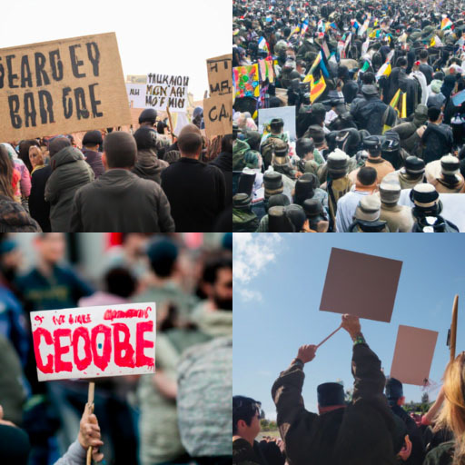
To verify the effectiveness of our data filters, we trained two GLIDE models with the same hyperparameters: one on unfiltered data, and one on the dataset after filtering. We refer to the former model as the unfiltered model, and the latter as the filtered model. As expected, we found that the unfiltered model generally produced less explicit or graphic content in response to requests for this kind of content. However, we also found an unexpected side-effect of data filtering: it created or amplified the model’s biases towards certain demographics.
Unfiltered
Filtered
Generations for the prompt “military protest” from our unfiltered model (left) and filtered model (right). Notably, the filtered model almost never produces images of guns.
Fixing Bias Introduced by Data Filters
Generative models attempt to match the distribution of their training data, including any biases therein. As a result, filtering the training data has the potential to create or amplify biases in downstream models. In general, fixing biases in the original dataset is a difficult sociotechnical task that we continue to study, and is beyond the scope of this post. The problem we address here is the amplification of biases caused specifically by data filtering itself. With our approach, we aim to prevent the filtered model from being more biased than the unfiltered model, essentially reducing the distribution shift caused by data filtering.
As a concrete example of bias amplification due to filtering, consider the prompt “a ceo”. When our unfiltered model generated images for this prompt, it tended to produce more images of men than women, and we expect that most of this bias is a reflection of our current training data. However, when we ran the same prompt through our filtered model, the bias appeared to be amplified; the generations were almost exclusively images of men.
We hypothesize that this particular case of bias amplification comes from two places: first, even if women and men have roughly equal representation in the original dataset, the dataset may be biased toward presenting women in more sexualized contexts; and second, our classifiers themselves may be biased either due to implementation or class definition, despite our efforts to ensure that this was not the case during the data collection and validation phases. Due to both of these effects, our filter may remove more images of women than men, which changes the gender ratio that the model observes in training.
To investigate filter-induced bias more thoroughly, we wanted a way to measure how much our data filters were affecting the bias towards various concepts. Notably, our violence and sexual content filters are purely image-based, but the multimodal nature of our dataset allows us to directly measure the effects of these filters on text. Since every image is accompanied by a text caption, we were able to look at the relative frequency of hand-selected keywords across the filtered and unfiltered dataset to estimate how much the filters were affecting any given concept.
To put this into practice, we used Apache Spark to compute the frequencies of a handful of keywords (e.g., “parent”, “woman”, “kid”) over all of the captions in both our filtered and unfiltered datasets. Even though our dataset contains hundreds of millions of text-image pairs, computing these keyword frequencies only took a few minutes using our compute cluster.
After computing keyword frequencies, we were able to confirm that our dataset filters had indeed skewed the frequencies of certain keywords more than others. For example, the filters reduced the frequency of the word “woman” by 14%, while the frequency of the word “man” was only reduced by 6%. This confirmed, on a large scale, what we had already observed anecdotally by sampling from GLIDE models trained on both datasets.
An illustration of dataset reweighting. We start with a balanced dataset (left). If our filter affects one category more than another, it can create a biased dataset (middle). Using reweighting, we effectively “repeat” some data more than others, allowing us to rebalance the bias caused by the filters (right).
Now that we had a proxy for measuring filter-induced bias, we needed a way to mitigate it. To tackle this problem, we aimed to re-weight the filtered dataset so that its distribution better matched the distribution of unfiltered images. As a toy example to illustrate this idea, suppose our dataset consists of 50% cat photos and 50% dog photos, but our data filters remove 75% of dogs but only 50% of cats. The final dataset would be ⅔ cats and ⅓ dogs, and a likelihood-based generative model trained on this dataset would likely generate more images of cats than dogs. We can fix this imbalance by multiplying the training loss of every image of a dog by 2, emulating the effect of repeating every dog image twice. It turns out that we can scale this approach to our real datasets and models in a way that is largely automatic–that is, we needn’t hand-select the features that we want to reweight.
We compute weights for images in the filtered dataset using probabilities from a special classifier, similar to the approach used by Choi et al. (2019). To train this classifier, we uniformly sample images from both datasets and predict which dataset the image came from. In particular, this model predicts P(unfiltered|image), given a prior P(unfiltered) = 0.5. In practice, we don’t want this model to be too powerful, or else it might learn the exact function implemented by our filters in the first place. Instead, we want the model to be smoother than our original data filters, capturing broad categories that are affected by the filters while still being unsure about whether a particular image would be filtered or not. To this end, we trained a linear probe on top of a small CLIP model.
Once we have a classifier which predicts the probability that an image is from the unfiltered dataset, we still need to convert this prediction into a weight for the image. For example, suppose that P(unfiltered|image) = 0.8. This means that the sample is 4 times more likely to be found in the unfiltered data than the filtered data, and a weight of 4 should correct the imbalance. More generally, we can use the weight P(unfiltered|image)/P(filtered|image).[1]
How well does this reweighting scheme actually mitigate the amplified bias? When we fine-tuned our previous filtered model with the new weighting scheme, the fine-tuned model’s behavior much more closely matched the unfiltered model on the biased examples we had previously found. While this was encouraging, we also wanted to evaluate this mitigation more thoroughly using our keyword-based bias heuristic. To measure keyword frequencies while taking our new weighting scheme into account, we can simply weight every instance of a keyword in the filtered dataset by the weight of the sample that contains it. Doing this, we get a new set of keyword frequencies that reflect the sample weights in the filtered dataset.
Across most of the keywords we checked, the reweighting scheme reduced the frequency change induced by filtering. For our previous examples of “man” and “woman”, the relative frequency reductions became 1% and –1%, whereas their previous values were 14% and 6%, respectively. While this metric is just a proxy for actual filtering bias, it is reassuring that our image-based reweighting scheme actually improves a text-based metric so significantly.
We are continuing to investigate remaining biases in DALL·E 2, in part through larger evaluations of the model’s behavior and investigations of how filtering impacted bias and capability development.
Preventing Image Regurgitation
We observed that our internal predecessors to DALL·E 2 would sometimes reproduce training images verbatim. This behavior was undesirable, since we would like DALL·E 2 to create original, unique images by default and not just “stitch together” pieces of existing images. Additionally, reproducing training images verbatim can raise legal questions around copyright infringement, ownership, and privacy (if people’s photos were present in training data).
To better understand the issue of image regurgitation, we collected a dataset of prompts that frequently resulted in duplicated images. To do this, we used a trained model to sample images for 50,000 prompts from our training dataset, and sorted the samples by perceptual similarity to the corresponding training image. Finally, we inspected the top matches by hand, finding only a few hundred true duplicate pairs out of the 50k total prompts. Even though the regurgitation rate appeared to be less than 1%, we felt it was necessary to push the rate down to 0 for the reasons stated above.
When we studied our dataset of regurgitated images, we noticed two patterns. First, the images were almost all simple vector graphics, which were likely easy to memorize due to their low information content. Second, and more importantly, the images all had many near-duplicates in the training dataset. For example, there might be a vector graphic which looks like a clock showing the time 1 o’clock—but then we would discover a training sample containing the same clock showing 2 o’clock, and then 3 o’clock, etc. Once we realized this, we used a distributed nearest neighbor search to verify that, indeed, all of the regurgitated images had perceptually similar duplicates in the dataset. Otherworks have observed a similar phenomenon in large language models, finding that data duplication is strongly linked to memorization.
The above finding suggested that, if we deduplicated our dataset, we might solve the regurgitation problem. To achieve this, we planned to use a neural network to identify groups of images that looked similar, and then remove all but one image from each group.[2] However, this would require checking, for each image, whether it is a duplicate of every other image in the dataset. Since our whole dataset contains hundreds of millions of images, we would naively need to check hundreds of quadrillions of image pairs to find all the duplicates. While this is technically within reach, especially on a large compute cluster, we found a much more efficient alternative that works almost as well at a small fraction of the cost.
Consider what happens if we cluster our dataset before performing deduplication. Since nearby samples often fall into the same cluster, most of the duplicate pairs would not cross cluster decision boundaries. We could then deduplicate samples within each cluster without checking for duplicates outside of the cluster, while only missing a small fraction of all duplicate pairs. This is much faster than the naive approach, since we no longer have to check every single pair of images.[3] When we tested this approach empirically on a small subset of our data, it found 85% of all duplicate pairs when using K=1024 clusters.
To improve the success rate of the above algorithm, we leveraged one key observation: when you cluster different random subsets of a dataset, the resulting cluster decision boundaries are often quite different. Therefore, if a duplicate pair crosses a cluster boundary for one clustering of the data, the same pair might fall inside a single cluster in a different clustering. The more clusterings you try, the more likely you are to discover a given duplicate pair. In practice, we settled on using five clusterings, which means that we search for duplicates of each image in the union of five different clusters. In practice, this found 97% of all duplicate pairs on a subset of our data.
Surprisingly, almost a quarter of our dataset was removed by deduplication. When we looked at the near-duplicate pairs that were found, many of them included meaningful changes. Recall the clock example from above: the dataset might include many images of the same clock at different times of day. While these images are likely to make the model memorize this particular clock’s appearance, they might also help the model learn to distinguish between times of day on a clock. Given how much data was removed, we were worried that removing images like this might have hurt the model’s performance.
To test the effect of deduplication on our models, we trained two models with identical hyperparameters: one on the full dataset, and one on the deduplicated version of the dataset. To compare the models, we used the same human evaluations we used to evaluate our original GLIDE model. Surprisingly, we found that human evaluators slightly preferred the model trained on deduplicated data, suggesting that the large amount of redundant images in the dataset was actually hurting performance.
Once we had a model trained on deduplicated data, we reran the regurgitation search we had previously done over 50k prompts from the training dataset. We found that the new model never regurgitated a training image when given the exact prompt for the image from the training dataset. To take this test another step further, we also performed a nearest neighbor search over the entire training dataset for each of the 50k generated images. This way, we thought we might catch the model regurgitating a different image than the one associated with a given prompt. Even with this more thorough check, we never found a case of image regurgitation.
Next Steps
While all of the mitigations discussed above represent significant progress towards our goal of reducing the risks associated with DALL·E 2, each mitigation still has room to improve:
Better pre-training filters could allow us to train DALL·E 2 on more data and potentially further reduce bias in the model. Our current filters are tuned for a low miss-rate at the cost of many false positives. As a result, we filtered out roughly 5% of our entire dataset even though most of these filtered images do not violate our content policy at all. Improving our filters could allow us to reclaim some of this training data.
Bias is introduced and potentially amplified at many stages of system development and deployment. Evaluating and mitigating the bias in systems like DALL·E 2 and the harm induced by this bias is an important interdisciplinary problem that we continue to study at OpenAI as part of our broader mission. Our work on this includes building evaluations to better understand the problem, curating new datasets, and applying techniques like human feedback and fine-tuning to build more robust and representative technologies.
It is also crucial that we continue to study memorization and generalization in deep learning systems. While deduplication is a good first step towards preventing memorization, it does not tell us everything there is to learn about why or how models like DALL·E 2 memorize training data.
Enterprises now have a new option for quickly getting started with NVIDIA AI software: the HPE GreenLake edge-to-cloud platform.
The NVIDIA AI Enterprise software suite is an end-to-end, cloud-native suite of AI and data analytics software. It’s optimized to enable any organization to use AI, and doesn’t require deep AI expertise.
Fully supported by NVIDIA, the software can be deployed anywhere, from the data center to the cloud. And developers can use the cloud-native platform of AI tools and frameworks to streamline development and deployment and quickly build high-performing AI solutions.
With NVIDIA AI Enterprise now available through HPE GreenLake in select countries, IT is relieved from the burden of building the infrastructure to run AI workloads. Organizations can access the NVIDIA AI Enterprise software suite as an on-prem cloud service from HPE, reducing the risk, duration, effort and cost for IT staff to build, deploy and operate an enterprise AI platform.
NVIDIA AI Enterprise is deployed on NVIDIA-Certified HPE ProLiant DL380 and DL385 servers running VMware vSphere with Tanzu. HPE GreenLake enables customers to acquire NVIDIA AI Enterprise on a pay-per-use basis, with the flexibility to scale up or down, and tailor to their needs. The software is fully supported by NVIDIA, ensuring robust operations for enterprise AI deployments.
HPE ProLiant DL380 and DL385 servers are optimized and certified with NVIDIA AI Enterprise software, VMware vSphere with Tanzu and NVIDIA A100 and A30 Tensor Core GPUs to deliver performance that is on par with bare metal for AI training and inference workloads.
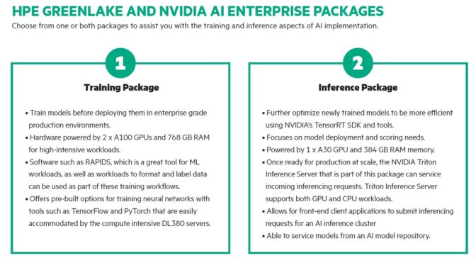
Customers can select from predefined packages for training or inference workloads. Packages include NVIDIA AI Enterprise software, NVIDIA Ampere architecture GPUs, VMware vSphere with Tanzu, as well as all setup, installation and configuration, including:
VMware ESXi and VMware vCenter installation
NVIDIA License System installation and configuration
NVIDIA AI Enterprise host software installation
NVIDIA AI Enterprise virtual machine creation and configuration
Data science and AI software installation
Validation
With HPE management services to monitor and manage infrastructure and public clouds, IT can free up resources for more strategic projects. Customers can also take advantage of HPE’s optional AI advisory and solutioning workshops, including AI use case design, implementation, testing and deployment.
The HPE GreenLake platform provides enterprises with centralized control and insights to manage resources, costs and capacity across their on-premises and cloud deployments with a secure, self-service provisioning and management via a common control pane.
Get immediate, short-term, remote access to try NVIDIA AI Enterprise now with NVIDIA LaunchPad. The program gives AI practitioners, data scientists and IT admins immediate access to NVIDIA AI with free hands-on labs featuring AI-powered chatbots, image classification and more.
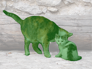
In computer vision, semantic segmentation is the task of classifying every pixel in an image with a class from a known set of labels such that pixels with the same label share certain characteristics. It generates a segmentation mask of the input images. For example, the following images show a segmentation mask of the cat label.
In November 2018, Amazon SageMaker announced the launch of the SageMaker semantic segmentation algorithm. With this algorithm, you can train your models with a public dataset or your own dataset. Popular image segmentation datasets include the Common Objects in Context (COCO) dataset and PASCAL Visual Object Classes (PASCAL VOC), but the classes of their labels are limited and you may want to train a model on target objects that aren’t included in the public datasets. In this case, you can use Amazon SageMaker Ground Truth to label your own dataset.
In this post, I demonstrate the following solutions:
Using Ground Truth to label a semantic segmentation dataset
Transforming the results from Ground Truth to the required input format for the SageMaker built-in semantic segmentation algorithm
Using the semantic segmentation algorithm to train a model and perform inference
Semantic segmentation data labeling
To build a machine learning model for semantic segmentation, we need to label a dataset at the pixel level. Ground Truth gives you the option to use human annotators through Amazon Mechanical Turk, third-party vendors, or your own private workforce. To learn more about workforces, refer to Create and Manage Workforces. If you don’t want to manage the labeling workforce on your own, Amazon SageMaker Ground Truth Plus is another great option as a new turnkey data labeling service that enables you to create high-quality training datasets quickly and reduces costs by up to 40%. For this post, I show you how to manually label the dataset with the Ground Truth auto-segment feature and crowdsource labeling with a Mechanical Turk workforce.
Manual labeling with Ground Truth
In December 2019, Ground Truth added an auto-segment feature to the semantic segmentation labeling user interface to increase labeling throughput and improve accuracy. For more information, refer to Auto-segmenting objects when performing semantic segmentation labeling with Amazon SageMaker Ground Truth. With this new feature, you can accelerate your labeling process on segmentation tasks. Instead of drawing a tightly fitting polygon or using the brush tool to capture an object in an image, you only draw four points: at the top-most, bottom-most, left-most, and right-most points of the object. Ground Truth takes these four points as input and uses the Deep Extreme Cut (DEXTR) algorithm to produce a tightly fitting mask around the object. For a tutorial using Ground Truth for image semantic segmentation labeling, refer to Image Semantic Segmentation. The following is an example of how the auto-segmentation tool generates a segmentation mask automatically after you choose the four extreme points of an object.
Crowdsourcing labeling with a Mechanical Turk workforce
If you have a large dataset and you don’t want to manually label hundreds or thousands of images yourself, you can use Mechanical Turk, which provides an on-demand, scalable, human workforce to complete jobs that humans can do better than computers. Mechanical Turk software formalizes job offers to the thousands of workers willing to do piecemeal work at their convenience. The software also retrieves the work performed and compiles it for you, the requester, who pays the workers for satisfactory work (only). To get started with Mechanical Turk, refer to Introduction to Amazon Mechanical Turk.
Create a labeling job
The following is an example of a Mechanical Turk labeling job for a sea turtle dataset. The sea turtle dataset is from the Kaggle competition Sea Turtle Face Detection, and I selected 300 images of the dataset for demonstration purposes. Sea turtle isn’t a common class in public datasets so it can represent a situation that requires labeling a massive dataset.
On the SageMaker console, choose Labeling jobs in the navigation pane.
Choose Create labeling job.
Enter a name for your job.
For Input data setup, select Automated data setup. This generates a manifest of input data.
For S3 location for input datasets, enter the path for the dataset.
For Task category, choose Image.
For Task selection, select Semantic segmentation.
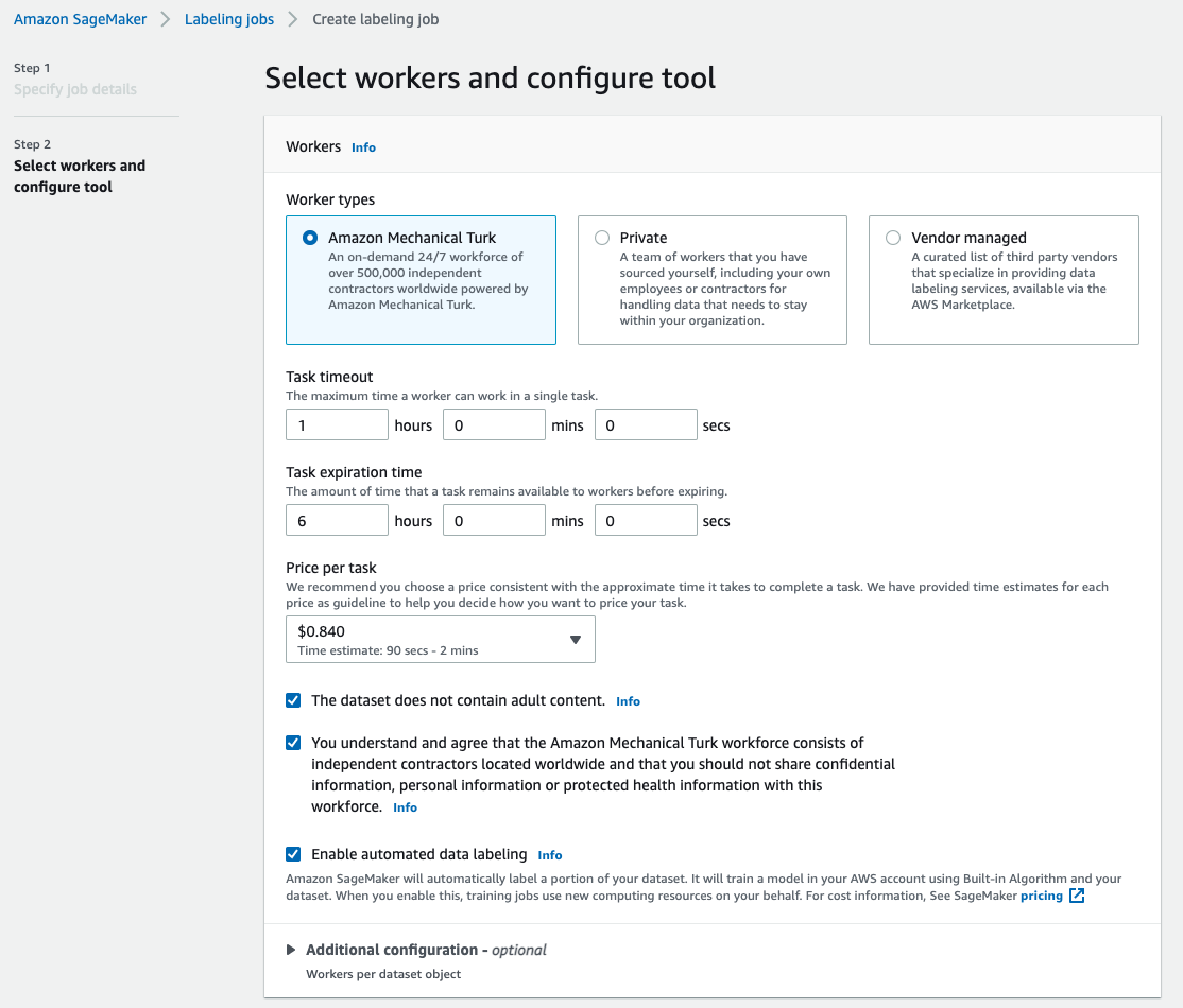
For Worker types, select Amazon Mechanical Turk.
Configure your settings for task timeout, task expiration time, and price per task.
Add a label (for this post, sea turtle), and provide labeling instructions.
Choose Create.
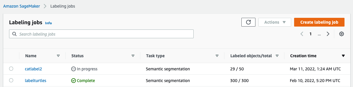
After you set up the labeling job, you can check the labeling progress on the SageMaker console. When it’s marked as complete, you can choose the job to check the results and use them for the next steps.
Dataset transformation
After you get the output from Ground Truth, you can use SageMaker built-in algorithms to train a model on this dataset. First, you need to prepare the labeled dataset as the requested input interface for the SageMaker semantic segmentation algorithm.
Requested input data channels
SageMaker semantic segmentation expects your training dataset to be stored on Amazon Simple Storage Service (Amazon S3). The dataset in Amazon S3 is expected to be presented in two channels, one for train and one for validation, using four directories, two for images and two for annotations. Annotations are expected to be uncompressed PNG images. The dataset might also have a label map that describes how the annotation mappings are established. If not, the algorithm uses a default. For inference, an endpoint accepts images with an image/jpeg content type. The following is the required structure of the data channels:
Every JPG image in the train and validation directories has a corresponding PNG label image with the same name in the train_annotation and validation_annotation directories. This naming convention helps the algorithm associate a label with its corresponding image during training. The train, train_annotation, validation, and validation_annotation channels are mandatory. The annotations are single-channel PNG images. The format works as long as the metadata (modes) in the image helps the algorithm read the annotation images into a single-channel 8-bit unsigned integer.
Output from the Ground Truth labeling job
The outputs generated from the Ground Truth labeling job have the following folder structure:
The segmentation masks are saved in s3://turtle2022/labelturtles/annotations/consolidated-annotation/output. Each annotation image is a .png file named after the index of the source image and the time when this image labeling was completed. For example, the following are the source image (Image_1.jpg) and its segmentation mask generated by the Mechanical Turk workforce (0_2022-02-10T17:41:04.724225.png). Notice that the index of the mask is different than the number in the source image name.
The output manifest from the labeling job is in the /manifests/output/output.manifest file. It’s a JSON file, and each line records a mapping between the source image and its label and other metadata. The following JSON line records a mapping between the shown source image and its annotation:
The source image is called Image_1.jpg, and the annotation’s name is 0_2022-02-10T17:41: 04.724225.png. To prepare the data as the required data channel formats of the SageMaker semantic segmentation algorithm, we need to change the annotation name so that it has the same name as the source JPG images. And we also need to split the dataset into train and validation directories for source images and the annotations.
Transform the output from a Ground Truth labeling job to the requested input format
To transform the output, complete the following steps:
Download all the files from the labeling job from Amazon S3 to a local directory:
Read the manifest file and change the names of the annotation to the same names as the source images:
import os
import re

label_job='labelturtles'
manifest_path=dir_name+'/'+label_job+'/'+'manifests/output/output.manifest'

file = open(manifest_path, "r")
txt=file.readlines()
output_path=dir_name+'/'+label_job+'/'+'annotations/consolidated-annotation/output'
S3_name='turtle2022/'
im_list=[]
for i in range(len(txt)):
    string = txt[i]
    try:
        im_name = re.search(S3_name+'(.+)'+'.jpg', string).group(1)
        print(im_name)
        im_png=im_name+'.png'
        im_list.append(im_name)
        annotation_name = re.search('output/(.+?)"', string).group(1)
        os.rename(annotation_name, im_png)
    except AttributeError:
        pass
Split the train and validation datasets:
import numpy as np
from random import sample

# Prints list of random items of given length
train_num=len(im_list)*0.8
test_num=len(im_list)*0.2
train_name=sample(im_list,int(train_num))
test_name = list(set(im_list) - set(train_name))
Make a directory in the required format for the semantic segmentation algorithm data channels:
Move the train and validation images and their annotations to the created directories.
For images, use the following code:
for i in range(len(train_name)):
    train_im=train_name[i]+'.jpg'
    train_im_path=dir_name+'/'+train_im
    train_new_path='train/'+train_im
    shutil.move(train_im_path,train_new_path)

    train_annotation=train_name[i]+'.png'
    train_annotation_path=dir_name+'/labelturtles/annotations/consolidated-annotation/output/'+train_annotation
    train_annotation_new_path='train_annotation/'+train_annotation
    shutil.move(train_annotation_path,train_annotation_new_path)
For annotations, use the following code:
for i in range(len(test_name)):
    val_im=test_name[i]+'.jpg'
    val_im_path=dir_name+'/'+val_im
    val_new_path='validation/'+val_im
    shutil.move(val_im_path,val_new_path)

    val_annotation=test_name[i]+'.png'
    val_annotation_path=dir_name+'/labelturtles/annotations/consolidated-annotation/output/'+val_annotation
    val_annotation_new_path='validation_annotationT/'+val_annotation
    shutil.move(val_annotation_path,val_annotation_new_path)
Upload the train and validation datasets and their annotation datasets to Amazon S3:
In this section, we walk through the steps to train your semantic segmentation model.
Follow the sample notebook and set up data channels
You can follow the instructions in Semantic Segmentation algorithm is now available in Amazon SageMaker to implement the semantic segmentation algorithm to your labeled dataset. This sample notebook shows an end-to-end example introducing the algorithm. In the notebook, you learn how to train and host a semantic segmentation model using the fully convolutional network (FCN) algorithm using the Pascal VOC dataset for training. Because I don’t plan to train a model from the Pascal VOC dataset, I skipped Step 3 (data preparation) in this notebook. Instead, I directly created train_channel, train_annotation_channe, validation_channel, and validation_annotation_channel using the S3 locations where I stored my images and annotations:
Adjust hyperparameters for your own dataset in SageMaker estimator
I followed the notebook and created a SageMaker estimator object (ss_estimator) to train my segmentation algorithm. One thing we need to customize for the new dataset is in ss_estimator.set_hyperparameters: we need to change num_classes=21 to num_classes=2 (turtle and background), and I also changed epochs=10 to epochs=30 because 10 is only for demo purposes. Then I used the p3.2xlarge instance for model training by setting instance_type="ml.p3.2xlarge". The training completed in 8 minutes. The best MIoU (Mean Intersection over Union) of 0.846 is achieved at epoch 11 with a pix_acc (the percent of pixels in your image that are classified correctly) of 0.925, which is a pretty good result for this small dataset.
Model inference results
I hosted the model on a low-cost ml.c5.xlarge instance:
Finally, I prepared a test set of 10 turtle images to see the inference result of the trained segmentation model:
import os

path = "testturtle/"
img_path_list=[]
files = os.listdir(path)

for file in files:

    if file.endswith(('.jpg', '.png', 'jpeg')):
        img_path = path + file
        img_path_list.append(img_path)

colnum=5
fig, axs = plt.subplots(2, colnum, figsize=(20, 10))

for i in range(len(img_path_list)):
    print(img_path_list[i])
    img = mpimg.imread(img_path_list[i])
    with open(img_path_list[i], "rb") as imfile:
        imbytes = imfile.read()
    cls_mask = ss_predictor.predict(imbytes)
    axs[int(i/colnum),i%colnum].imshow(img, cmap='gray')
    axs[int(i/colnum),i%colnum].imshow(np.ma.masked_equal(cls_mask,0), cmap='jet', alpha=0.8)

plt.show()
The following images show the results.
The segmentation masks of the sea turtles look accurate and I’m happy with this result trained on a 300-image dataset labeled by Mechanical Turk workers. You can also explore other available networks such as pyramid-scene-parsing network (PSP) or DeepLab-V3 in the sample notebook with your dataset.
Clean up
Delete the endpoint when you’re finished with it to avoid incurring continued costs:
ss_predictor.delete_endpoint()
Conclusion
In this post, I showed how to customize semantic segmentation data labeling and model training using SageMaker. First, you can set up a labeling job with the auto-segmentation tool or use a Mechanical Turk workforce (as well as other options). If you have more than 5,000 objects, you can also use automated data labeling. Then you transform the outputs from your Ground Truth labeling job to the required input formats for SageMaker built-in semantic segmentation training. After that, you can use an accelerated computing instance (such as p2 or p3) to train a semantic segmentation model with the following notebook and deploy the model to a more cost-effective instance (such as ml.c5.xlarge). Lastly, you can review the inference results on your test dataset with a few lines of code.
Get started with SageMaker semantic segmentation data labeling and model training with your favorite dataset!
About the Author
Kara Yang is a Data Scientist in AWS Professional Services. She is passionate about helping customers achieve their business goals with AWS cloud services. She has helped organizations build ML solutions across multiple industries such as manufacturing, automotive, environmental sustainability and aerospace.