How Computational Graphs are Executed in PyTorch

Welcome to the last entry into understanding the autograd engine of PyTorch series!
If you haven’t read parts 1 & 2 check them now to understand how PyTorch creates the computational graph for the backward pass!

This post is based on PyTorch v1.11, so some highlighted parts may differ across versions.

PyTorch autograd graph execution

The last post showed how PyTorch constructs the graph to calculate the outputs’ derivatives w.r.t. the inputs when executing the forward pass. Now we will see how the execution of the backward pass is coordinated and done by looking at the whole process, starting from Python down to the lower C++ level internals.

What Happens when Calling backward()/grad() from Python

Using variable.backward()

After doing all our calculations with an input set to require the gradient, we call .backward() on the result to initiate the backward pass execution.

>>> x = torch.tensor([0.5, 0.75], requires_grad=True)
>>> y = torch.exp(x).sum()
>>> y.backward()

Calling .backward() on a tensor results in a call to torch.autograd.backward().

# torch/_tensor.py

def backward(self, gradient=None, retain_graph=None, create_graph=False, inputs=None):
    
    torch.autograd.backward(self, gradient, retain_graph, create_graph, inputs=inputs)

torch.autograd.backward() checks the arguments and calls the autograd engine in the C++ layer.

def backward(
    tensors: _TensorOrTensors,
    grad_tensors: Optional[_TensorOrTensors] = None,
    retain_graph: Optional[bool] = None,
    create_graph: bool = False,
    grad_variables: Optional[_TensorOrTensors] = None,
    inputs: Optional[_TensorOrTensors] = None,
) -> None:
    

    if inputs is not None and len(inputs) == 0:
        raise RuntimeError("'inputs' argument to backward() cannot be empty.")

    tensors = (tensors,) if isinstance(tensors, torch.Tensor) else tuple(tensors)
    inputs = (inputs,) if isinstance(inputs, torch.Tensor) else 
        tuple(inputs) if inputs is not None else tuple()

    grad_tensors_ = _tensor_or_tensors_to_tuple(grad_tensors, len(tensors))
    grad_tensors_ = _make_grads(tensors, grad_tensors_)
    if retain_graph is None:
        retain_graph = create_graph

    Variable._execution_engine.run_backward(
        tensors, grad_tensors_, retain_graph, create_graph, inputs,
        allow_unreachable=True, accumulate_grad=True)  # allow_unreachable flag

First, whether the grad_tensors argument was specified or not, there is a call to the _make_grads function. This is used to check the provided grad_tensors or to specify the default value for them by looking at the tensors argument values’ shapes. Check the first blog post for details on the default value for the grad_tensors of the backward pass. This function just provides the vector of the vector jacobian product if it was not initially specified.

In the above code, Variable has an _execution_engine attribute that is defined in torch.autograd.variable to be of type ImperativeEngine; the C++ engine exported to python and declared in torch/csrc/autograd/python_engine.cpp. In the following sections, we explain in detail how this object executes the backward pass.

Note that the torch.autograd.backward function has an inputs optional argument. This argument is used when we want to calculate the .grad field of only a subset of input tensors in the forward pass.

>>> x = torch.tensor([0.5, 0.75], requires_grad=True)
>>> y = torch.tensor([0.1, 0.90], requires_grad=True)
>>> z = torch.exp(x * y).sum()
>>> torch.autograd.backward([z], inputs=[x])
>>> x.grad
tensor([0.1051, 1.7676])
>>> y.grad  # None
>>>

Using torch.autograd.grad

An alternative to backward() is to use torch.autograd.grad(). The main difference to backward() is that grad() returns a tuple of tensors with the gradients of the outputs w.r.t. the inputs kwargs instead of storing them in the .grad field of the tensors. As you can see, the grad() code shown below is very similar to backward.

def grad(
    outputs: _TensorOrTensors,
    inputs: _TensorOrTensors,
    grad_outputs: Optional[_TensorOrTensors] = None,
    retain_graph: Optional[bool] = None,
    create_graph: bool = False,
    only_inputs: bool = True,
    allow_unused: bool = False,
   is_grads_batched: bool = False
) -> Tuple[torch.Tensor, ...]:
   
    outputs = (outputs,) if isinstance(outputs, torch.Tensor) else tuple(outputs)
    inputs = (inputs,) if isinstance(inputs, torch.Tensor) else tuple(inputs)
    overridable_args = outputs + inputs
    if has_torch_function(overridable_args):
        return handle_torch_function(
            grad,
            overridable_args,
            outputs,
            inputs,
            grad_outputs=grad_outputs,
            retain_graph=retain_graph,
            create_graph=create_graph,
            only_inputs=only_inputs,
            allow_unused=allow_unused,
        )

    grad_outputs_ = _tensor_or_tensors_to_tuple(grad_outputs, len(outputs))
    grad_outputs_ = _make_grads(outputs, grad_outputs_)

    if retain_graph is None:
        retain_graph = create_graph

    if is_grads_batched:
        # …. It will not be covered here
    else:
        return Variable._execution_engine.run_backward(
            outputs, grad_outputs_, retain_graph, create_graph, inputs,
            allow_unused, accumulate_grad=False)  # Calls into the C++ engine to run the backward pass

Figure 1 shows the computational graph with the backward() and grad() arguments highlighted in red and blue, respectively:

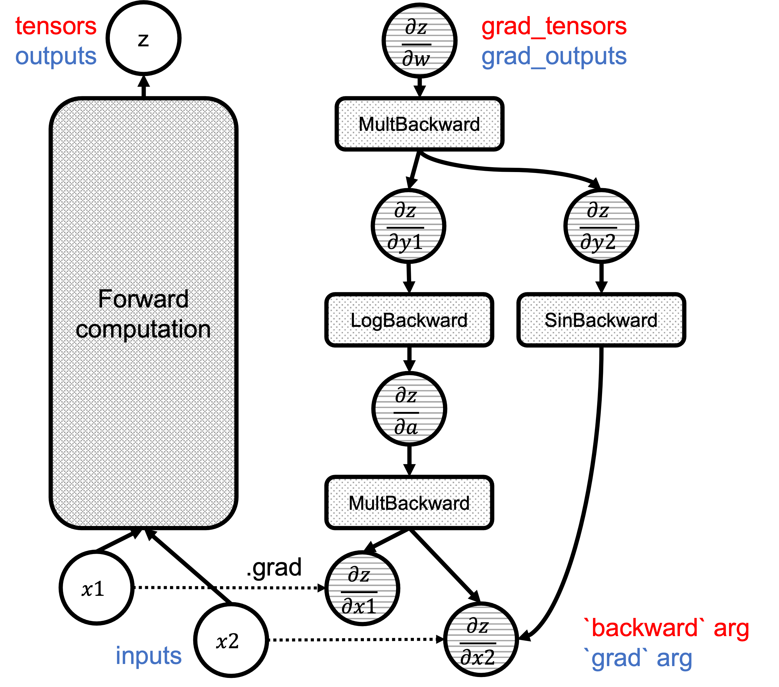
Fgiure 1: Correspondence of `backward`/`grad` arguments in the graphs.

Going Inside the Autograd Engine

Refreshing Concepts: Nodes and Edges

As we saw in 2
The computational graph comprises Node and Edge objects. Please read that post if you haven’t done it yet.

Nodes

Node objects are defined in torch/csrc/autograd/function.h, and they provide an overload of operator() for the associated function and a list of edges to do the graph traversal. Note that Node is a base class that autograd functions inherit from and override the apply method to execute the backward function.

struct TORCH_API Node : std::enable_shared_from_this<Node> {
 ...
 /// Evaluates the function on the given inputs and returns the result of the
  /// function call.
  variable_list operator()(variable_list&& inputs) {
  ...
  }

protected:
  /// Performs the `Node`'s actual operation.
  virtual variable_list apply(variable_list&& inputs) = 0;
  
  edge_list next_edges_;
  uint64_t topological_nr_ = 0;
  

There is an attribute called topological_nr_ in every node object. This number is used to optimize the graph execution as it allows to discard of graph branches under certain conditions. The topological number is the longest distance between this node and any leaf node and it is shown in Figure 2. Its main property is that for any pair of nodes x, y in a directed graph topo_nr(x) < topo_nr(y) means that there is no path from x to y. So this allows for reducing the number of paths in the graph in need of traversal. Check the topological_nr
) method comment for further details.

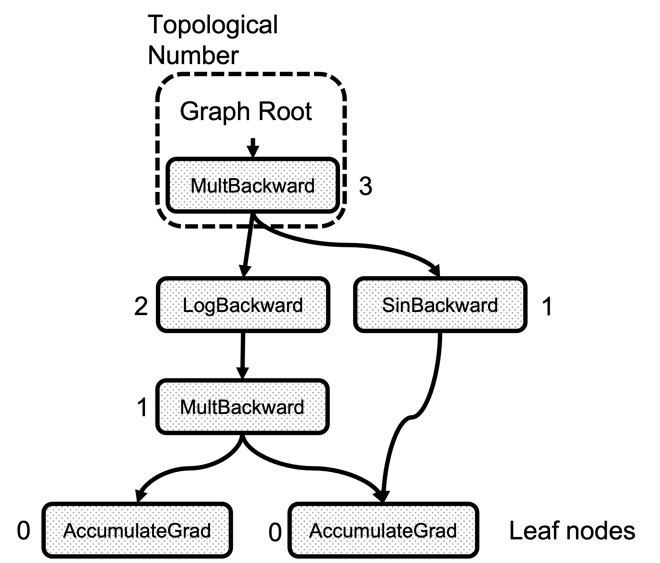
Figure 2: Example of the Topological Number calculation

Edges

The Edge object links Nodes together, and its implementation is straightforward.

struct Edge {
  ...
  /// The function this `Edge` points to.
  std::shared_ptr<Node> function;
  /// The identifier of a particular input to the function.
  uint32_t input_nr;
};

It only requires a function pointer to the Node and an input number that is the index of the output from the forward function this edge points to. When preparing the set of gradients before calling “function”, we know that what is flowing from this edge should be accumulated in the “input_nr”th argument. Note that the input/output name is flipped here and this is the input to the backward function.
Edge objects are constructed using the gradient_edge function method.

 Edge gradient_edge(const Variable& self) {
    if (const auto& gradient = self.grad_fn()) {
      return Edge(gradient, self.output_nr());
    } else {
      return Edge(grad_accumulator(self), 0);
    }
  }

Entering the C++ Realm

Once that torch.autograd.backward() has been invoked, the
THPEngine_run_backward routine starts the graph traversal. Following is a schema of the function body:

PyObject *THPEngine_run_backward(PyObject *self, PyObject *args, PyObject *kwargs)
{
  HANDLE_TH_ERRORS
  PyObject *tensors = nullptr;
  PyObject *grad_tensors = nullptr;
  unsigned char keep_graph = 0;
  unsigned char create_graph = 0;
  PyObject *inputs = nullptr;
  
  // Convert the python arguments to C++ objects
  const char *accepted_kwargs[] = { // NOLINT
      "tensors", "grad_tensors", "keep_graph", "create_graph", "inputs",
      "allow_unreachable", "accumulate_grad", nullptr
  };
  if (!PyArg_ParseTupleAndKeywords(args, kwargs, "OObb|Obb", (char**)accepted_kwargs,
        &tensors, &grad_tensors, &keep_graph, &create_graph, &inputs, &allow_unreachable, &accumulate_grad))

 // Prepare arguments
 for(const auto i : c10::irange(num_tensors)) {
   // Check that the tensors require gradients
  }

  std::vector<Edge> output_edges;
  if (inputs != nullptr) {
     // Prepare outputs
  }

  {
      // Calls the actual autograd engine
    pybind11::gil_scoped_release no_gil;
    outputs = engine.execute(roots, grads, keep_graph, create_graph, accumulate_grad, output_edges);
  }
    // Clean up and finish
}

First, we prepare the input arguments after converting the PyObject arguments to actual C++ objects. The tensors list contains the tensors from which we start the backward pass. These tensors are converted to edges using torch::autograd::impl::gradient_edge and added to a list called roots where the graph traversal starts.

 edge_list roots;
  roots.reserve(num_tensors);
  variable_list grads;
  grads.reserve(num_tensors);
  for(const auto i : c10::irange(num_tensors)) {
    PyObject *_tensor = PyTuple_GET_ITEM(tensors, i);
       const auto& variable = THPVariable_Unpack(_tensor);
       auto gradient_edge = torch::autograd::impl::gradient_edge(variable);
     roots.push_back(std::move(gradient_edge));

    PyObject *grad = PyTuple_GET_ITEM(grad_tensors, i);
    if (THPVariable_Check(grad)) {
      const Variable& grad_var = THPVariable_Unpack(grad);
      grads.push_back(grad_var);
    } 
  }

Now, if the inputs argument was specified in backward or we used the torch.autograd.grad api, the following code creates a list of edges to accumulate the gradients in the specified tensors at the end of the computation. The engine uses this later to optimize the execution as it doesn’t add the gradients in all the leaf nodes, just the specified ones.

  std::vector<Edge> output_edges;
  if (inputs != nullptr) {
    int num_inputs = PyTuple_GET_SIZE(inputs);
    output_edges.reserve(num_inputs);
    for (const auto i : c10::irange(num_inputs)) {
      PyObject *input = PyTuple_GET_ITEM(inputs, i);
      const auto& tensor = THPVariable_Unpack(input);
      const auto output_nr = tensor.output_nr();
      auto grad_fn = tensor.grad_fn();
      if (!grad_fn) {
        grad_fn = torch::autograd::impl::try_get_grad_accumulator(tensor);
      }
      if (accumulate_grad) {
        tensor.retain_grad();
      }
      if (!grad_fn) {
        output_edges.emplace_back(std::make_shared<Identity>(), 0);
      } else {
        output_edges.emplace_back(grad_fn, output_nr);
      }
    }
  }

The next step is the actual graph traversal and node function execution, and finally, the cleanup and return.

  {
    // Calls the actual autograd engine
    pybind11::gil_scoped_release no_gil;
    auto& engine = python::PythonEngine::get_python_engine();
    outputs = engine.execute(roots, grads, keep_graph, create_graph, accumulate_grad, output_edges);
  }
  // Clean up and finish
}

Starting the Real Execution

engine.executeis present in torch/csrc/autograd/engine.cpp

There are two differentiated steps here:

Analyze the graph to find dependencies between functions
Create worker threads that traverse the graph

Data Structures Used for the Execution

GraphTask

All the execution metadata is managed by the GraphTask class in torch/csrc/autograd/engine.h

struct GraphTask: std::enable_shared_from_this<GraphTask> {
  std::atomic<uint64_t> outstanding_tasks_{0};
  //  … 
  std::unordered_map<Node*, InputBuffer> not_ready_;
  std::unordered_map<Node*, int> dependencies_;

  struct ExecInfo {
     // …
  };
  std::unordered_map<Node*, ExecInfo> exec_info_;
  std::vector<Variable> captured_vars_;
  // …
  std::shared_ptr<ReadyQueue> cpu_ready_queue_;
};

Here we see a series of variables dedicated to maintaining the execution state.
outstanding_tasks_ tracks the number of tasks left to be executed for the backward pass to complete. not_ready_ holds the input arguments for the Nodes that are not ready to be executed. dependencies_ track the number of predecessors that a Node has. As the count reaches 0, the Node is ready for execution; it is placed in a ready queue to be retrieved and executed later.

exec_info_ and the associated ExecInfo struct are used only when the inputs argument is specified or it is a call to autograd.grad(). They allow filter paths on the graph that are not needeed since only the gradients are calculated only for the variables in the inputs list.

captured_vars_ is where the results of the graph execution are temporarily stored if we used the torch.autograd.grad() api instead of torch.autograd.backward() since grad() returns the gradients as tensors instead of just filling the .grad field of the inputs.

NodeTask

The NodeTask struct is a basic class that holds an fn_ pointer to the node to execute, and an inputs_ buffer to store the input arguments to this function. Note that the functions executed by the backward pass are the derivatives specified in the derivatives.yaml file. or the user provided backward function when using custom functions as described in the second blog post.

The inputs_ buffer is also where the output gradients of the previously executed functions are aggregated, and it is defined as a std::vector<Variable> container with facilities to accumulate values at a given position.

struct NodeTask {
  std::weak_ptr<GraphTask> base_;
  std::shared_ptr<Node> fn_;
  // This buffer serves as an implicit "addition" node for all of the
  // gradients flowing here.  Once all the dependencies are finished, we
  // use the contents of this buffer to run the function.
  InputBuffer inputs_;
};

GraphRoot

The GraphRoot is a special function used to hold multiple input variables in a single place. The code is pretty simple as it only acts as a container of variables.

struct TORCH_API GraphRoot : public Node {
  GraphRoot(edge_list functions, variable_list inputs)
      : Node(std::move(functions)),
      outputs(std::move(inputs)) {
    for (const auto& t : outputs) {
      add_input_metadata(t);
    }
  }

  variable_list apply(variable_list&& inputs) override {
    return outputs;
  }

AccumulateGrad

This function is set during the graph creation in gradient_edge when the Variable object doesn’t have a grad_fn. This is, it is a leaf node.

    if (const auto& gradient = self.grad_fn()) {
      // …
    } else {
      return Edge(grad_accumulator(self), 0);
    }

The function body is defined in torch/csrc/autograd/functions/accumulate_grad.cpp and it essentially accumulates the input grads in the object’s .grad attribute.

auto AccumulateGrad::apply(variable_list&& grads) -> variable_list {
  check_input_variables("AccumulateGrad", grads, 1, 0);
  

  at::Tensor new_grad = callHooks(variable, std::move(grads[0]));
  std::lock_guard<std::mutex> lock(mutex_);

  at::Tensor& grad = variable.mutable_grad();
  accumulateGrad(
      variable,
      grad,
      new_grad,
      1 + !post_hooks().empty() /* num_expected_refs */,
      [&grad](at::Tensor&& grad_update) { grad = std::move(grad_update); });
  return variable_list();
}
}} // namespace torch::autograd


accumulateGrad
does several checks on the tensors format and eventually performs the variable_grad += new_grad; accumulation.

Preparing the graph for execution

Now, let’s walk through Engine::execute. The first thing to do besides arguments consistency checks is to create the actual GraphTask object we described above. This object keeps all the metadata of the graph execution.

auto Engine::execute(const edge_list& roots,
                     const variable_list& inputs,
                     bool keep_graph,
                     bool create_graph,
                     bool accumulate_grad,
                     const edge_list& outputs) -> variable_list {

  validate_outputs(roots, const_cast<variable_list&>(inputs), [](const std::string& msg) {
    return msg;
  });

  // Checks

  auto graph_task = std::make_shared<GraphTask>(
      /* keep_graph */ keep_graph,
      /* create_graph */ create_graph,
      /* depth */ not_reentrant_backward_call ? 0 : total_depth + 1,
      /* cpu_ready_queue */ local_ready_queue);

  // If we receive a single root, skip creating extra root node
  // …
  // Prepare graph by computing dependencies
  // …
  // Queue the root 
  // …
  // launch execution
  // …
}

After creating the GraphTask, we use its associated function if we only have one root node. If we have multiple root nodes, we create a special GraphRoot object as described before.

  bool skip_dummy_node = roots.size() == 1;
  auto graph_root = skip_dummy_node ?
    roots.at(0).function :
    std::make_shared<GraphRoot>(roots, inputs);

The next step is to fill the dependencies_ map in the GraphTask object since the engine must know when it can execute a task. The outputs here is the inputs argument passed to the torch.autograd.backward() call in Python. But here, we have reversed the names since the gradients w.r.t. the inputs of the forward pass are now the outputs of the backward pass. And from now on, there is no concept of forward/backward, but only graph traversal and execution.

  auto min_topo_nr = compute_min_topological_nr(outputs);
  // Now compute the dependencies for all executable functions
  compute_dependencies(graph_root.get(), *graph_task, min_topo_nr);

  if (!outputs.empty()) {
    graph_task->init_to_execute(*graph_root, outputs, accumulate_grad, min_topo_nr);
  }

Here we preprocess the graph for the execution of the nodes. First, compute_min_topological_nr is called to to obtain the minimum topological number of the tensors specified in outputs (0 if no inputs kwarg was supplied to .backward or input for .grad). This computation prunes paths in the graph that lead to input variables of which we don’t want/need to calculate the grads.

Second, is the compute_dependencies call. This function is a very simple graph traversal that starts with the root Node, and for each of the edges in node.next_edges() it increments the counter in dependencies_. Figure 3 shows the result of the dependencies calculation for the example graph. Note that the number of dependencies of any node is just the number of edges arriving at it.

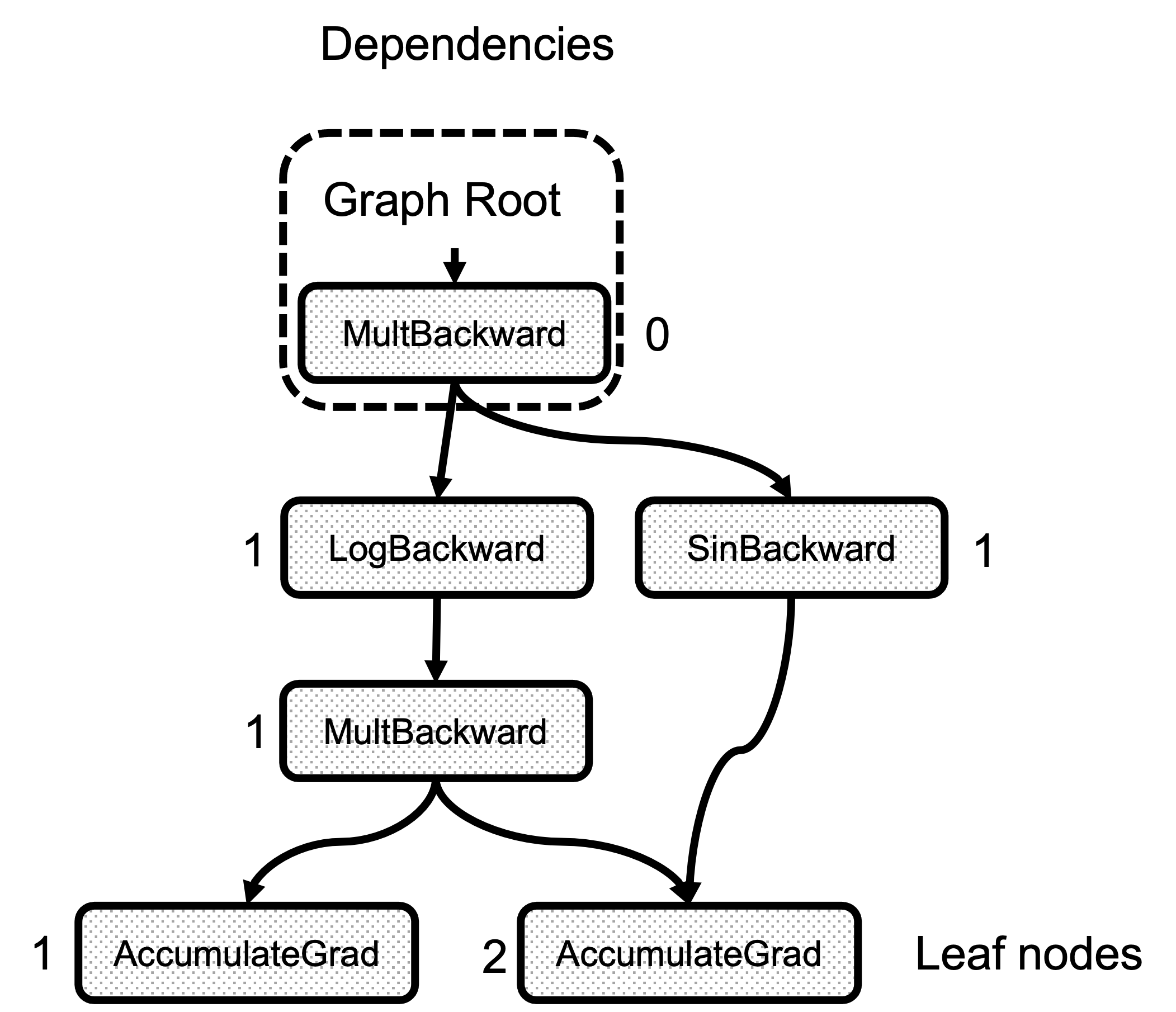
Figure 3: Number of dependencies for each node

Finally, the init_to_execute call, this is the one that populates the GraphTask::exec_info_ map in case that inputs were specified in the python backward call. It iterates the graph again, starting from the root, and records in the exec_info_ map the intermediate nodes needed to calculate only the given inputs gradients.

  // Queue the root
  if (skip_dummy_node) {
    InputBuffer input_buffer(roots.at(0).function->num_inputs());
    auto input = inputs.at(0);


    input_buffer.add(roots.at(0).input_nr,
                      std::move(input),
                      input_stream,
                      opt_next_stream);

    execute_with_graph_task(graph_task, graph_root, std::move(input_buffer));
  } else {
    execute_with_graph_task(graph_task, graph_root, InputBuffer(variable_list()));
  }
  // Avoid a refcount bump for the Future, since we check for refcount in
  // DistEngine (see TORCH_INTERNAL_ASSERT(futureGrads.use_count() == 1)
  // in dist_engine.cpp).
  auto& fut = graph_task->future_result_;
  fut->wait();
  return fut->value().toTensorVector();
}

And now, we are ready to start the actual execution by creating the InputBuffer. In case we only have one root variable, we begin by copying the value of the inputs tensor (this is the gradients passed to python backward) in position 0 of the input_buffer. This is a small optimization that avoids running the RootNode for no reason. Also, if the rest of the graph is not on the cpu, we directly start on that worker while the RootNode is always placed on the cpu ready queue. Details of the workers and ready queues are explained in the section below.

On the other hand, if we have multiple roots, the GraphRoot object also holds the inputs, so it is enough to pass it an empty InputBuffer.

Graph Traversal and Node Execution

Devices, Threads and Queues

Before diving into the actual execution, we need to see how the engine is structured.

First of all, the engine is multithreaded with one thread per device. For example, the caller thread is associated with the CPU while additional threads are created and associated with each GPU or other devices available in the system. Each thread tracks its device using thread-local storage in the worker_device variable. In addition, the threads have a queue of tasks to be executed also located in thread-local storage, the local_ready_queue. This is where work is queued for this thread to execute in the thread_main function that is explained later.
You will wonder how the device where a task should be executed is decided. The InputBuffer class has a device() function that returns the first non-cpu device of all its tensors.
This function is used together with Engine::ready_queue to select the queue to queue a task.

auto Engine::ready_queue(std::shared_ptr<ReadyQueue> cpu_ready_queue, at::Device device) -> std::shared_ptr<ReadyQueue>{
  if (device.type() == at::kCPU || device.type() == at::DeviceType::Meta) {
    return cpu_ready_queue;
  } else {
    // See Note [Allocating GPUs to autograd threads]
    return device_ready_queues_.at(device.index());
  }
}

The ReadyQueue object is defined in torch/csrc/autograd/engine.h and it is a simple wrapper over std::priority_queue that allows a thread to wait for a task if it’s empty. One interesting property of the ReadyQueue is that it increases the GraphTask::outstanding_tasks_ value used to determine if the execution has completed or not.

auto ReadyQueue::push(NodeTask item, bool incrementOutstandingTasks) -> void {
  {
    std::lock_guard<std::mutex> lock(mutex_);
    if (incrementOutstandingTasks) {
      std::shared_ptr<GraphTask> graph_task = item.base_.lock();
      ++graph_task->outstanding_tasks_;
    }
    heap_.push(std::move(item));
  }
  not_empty_.notify_one();
}

auto ReadyQueue::pop() -> NodeTask {
  std::unique_lock<std::mutex> lock(mutex_);
  not_empty_.wait(lock, [this]{ return !heap_.empty(); });
  auto task = std::move(const_cast<NodeTask&>(heap_.top())); heap_.pop();
  return task;
}

Reentrant Backward

A reentrant backward happens when one of the tasks in a backward pass calls again backward. It is not a very common case, but it can be used to reduce memory utilization as it could potentially avoid saving intermediate results. For more information, check this PyTorch forum post.

class ReentrantBackward(torch.autograd.Function):
    @staticmethod
    def forward(ctx, input):
        return input.sum()

    @staticmethod
    def backward(ctx, input):
        # Let's compute the backward by using autograd
        input = input.detach().requires_grad_()
        with torch.enable_grad():
            out = input.sum()
        out.backward()  # REENTRANT CALL!!
        return out.detach()

Here, we call backward() inside backward() for a user custom-defined autograd function.
This situation can lead to deadlocks because the first backward needs to wait for the second one to complete. But some internal implementation details can prevent the second backward from completing as it is explained in the dedicated subsection.

Thread Initialization

execute_with_graph_task is in charge of initializing the threads taking care of the computation and placing the root node in the queue of the device that produced it.

c10::intrusive_ptr<at::ivalue::Future> Engine::execute_with_graph_task(
    const std::shared_ptr<GraphTask>& graph_task,
    std::shared_ptr<Node> graph_root,
    InputBuffer&& input_buffer) {

  initialize_device_threads_pool();
  // Lock mutex for GraphTask.
  std::unique_lock<std::mutex> lock(graph_task->mutex_);

  auto queue = ready_queue(graph_task->cpu_ready_queue_, input_buffer.device());

  if (worker_device == NO_DEVICE) {
    set_device(CPU_DEVICE);
    graph_task->owner_ = worker_device;
    queue->push(NodeTask(graph_task, std::move(graph_root), std::move(input_buffer)));
    lock.unlock();
    thread_main(graph_task);
    worker_device = NO_DEVICE;
  } else {
     // This deals with reentrant backwards, we will see it later.
  }
  return graph_task->future_result_;
}

First, this function initializes several threads (one per device) calling initialize_device_threads_pool() where several things happen:
One ReadyQueue per device is created.
One thread per non-cpu device is created.
A thread local worker_device variable is set to track the current device associated with the thread.
thread_main function is called, and threads wait for tasks to be put in their queues.

Then it retrieves the queue to place the root node based on the device that holds the tensors present in the input_buffer using the ready_queue function. Now, the main thread (the one also executing the Python interpreter) has its worker_device set to NO_DEVICE, and it is in charge of executing functions with all its tensors living in the cpu. If worker_device is set to any other value, the graph execution is already started, and .backward() was called inside a running Node, creating a reentrant backward call. This is explained later. For now,
the main thread places the task in the queue and call thread_main.

Where the Magic Happens

It’s been a long way, but finally, we are ready to traverse the graph and execute the nodes. Each of the spawned threads, and the main thread call thread_main.

auto Engine::thread_main(const std::shared_ptr<GraphTask>& graph_task) -> void {

  while (graph_task == nullptr || !graph_task->future_result_->completed()) {
    std::shared_ptr<GraphTask> local_graph_task;
    {
      NodeTask task = local_ready_queue->pop();

      if (task.isShutdownTask_) {
        break;
      }

      if (!(local_graph_task = task.base_.lock())) {
        // GraphTask for function is no longer valid, skipping further
        // execution.
        continue;
      }

      if (task.fn_ && !local_graph_task->has_error_.load()) {
        at::ThreadLocalStateGuard tls_guard(local_graph_task->thread_locals_);

        try {
          GraphTaskGuard guard(local_graph_task);
          NodeGuard ndguard(task.fn_);
          {
            evaluate_function(
                local_graph_task,
                task.fn_.get(),
                task.inputs_,
                local_graph_task->cpu_ready_queue_);
          }
        } catch (std::exception& e) {
          thread_on_exception(local_graph_task, task.fn_, e);
        }
      }
    }

    // Decrement the outstanding tasks.
    --local_graph_task->outstanding_tasks_;

    // Check if we've completed execution.
    if (local_graph_task->completed()) {
      local_graph_task->mark_as_completed_and_run_post_processing();
      auto base_owner = local_graph_task->owner_;
      if (worker_device != base_owner) {
        std::atomic_thread_fence(std::memory_order_release);
        ready_queue_by_index(local_graph_task->cpu_ready_queue_, base_owner)
            ->push(NodeTask(local_graph_task, nullptr, InputBuffer(0)));
      }
    }
  }
}

The code here is simple, given the local_ready_queue assigned to each thread in thread-local storage. The threads loop until there are no tasks left to execute in the graph. Note that for device-associated threads, the passed graph_task argument is nullptr, and they block in local_ready_queue->pop() until a task is pushed in their queue. After some consistency checks (the task type is shutdown, or the graph is still valid). We get to the actual function invocation in evaluate_function.

        try {
          GraphTaskGuard guard(local_graph_task);
          NodeGuard ndguard(task.fn_);
          {
            evaluate_function(
                local_graph_task,
                task.fn_.get(),
                task.inputs_,
                local_graph_task->cpu_ready_queue_);
          }
        } catch (std::exception& e) {
          thread_on_exception(local_graph_task, task.fn_, e);
        }
      }

After calling evaluate_function, we check if the graph_task execution is complete by looking the outstanding_tasks_ number. This number increases when a task is pushed to a queue and is decreased in local_graph_task->completed() when a task is executed. When the execution is done, we return the results that are be in the captured_vars_ in case we called torch.autograd.grad() instead of torch.autograd.backward() as this function returns tensors instead of storing them in the .grad attribute of the inputs. Finally we wake up the main thread if it’s waiting by sending a dummy task.

   // Decrement the outstanding tasks.
    --local_graph_task->outstanding_tasks_;

    // Check if we've completed execution.
    if (local_graph_task->completed()) {
      local_graph_task->mark_as_completed_and_run_post_processing();
      auto base_owner = local_graph_task->owner_;
      if (worker_device != base_owner) {
        std::atomic_thread_fence(std::memory_order_release);
        ready_queue_by_index(local_graph_task->cpu_ready_queue_, base_owner)
            ->push(NodeTask(local_graph_task, nullptr, InputBuffer(0)));
      }
    }

Calling the Function and Unlocking New Tasks

evaluate_function serves three purposes:

Run the function.
Accumulate its results in the next node InputBuffers.
Decrease the dependencies counter of the next nodes and enqueues the tasks reaching 0 to be executed.

void Engine::evaluate_function(
    std::shared_ptr<GraphTask>& graph_task,
    Node* func,
    InputBuffer& inputs,
    const std::shared_ptr<ReadyQueue>& cpu_ready_queue) {

  // If exec_info_ is not empty, we have to instrument the execution
  auto& exec_info_ = graph_task->exec_info_;
  if (!exec_info_.empty()) {
    // Checks if the function needs to be executed 
    if (!fn_info.needed_) {
      // Skip execution if we don't need to execute the function.
      return;
    }
  }

  auto outputs = call_function(graph_task, func, inputs);

  auto& fn = *func;
  if (!graph_task->keep_graph_) {
    fn.release_variables();
  }

Initially, we check the exec_info_ map of the GraphTask structure to determine if the current node needs to be executed. Remember that if this map is empty, all the nodes are executed because we are calculating the grads for all the inputs of the forward pass.

After this check, the function is executed by running call_function. Its implementation is very straightforward and calls the actual derivative function and registered hooks if any.

  int num_outputs = outputs.size();
  if (num_outputs == 0) {
    // Records leaf stream (if applicable)
    return;
  }

  if (AnomalyMode::is_enabled()) {
    // check for nan values in result
  }

Next, we check the outputs of the function after call_function is done. If the number of outputs is 0, there are no following nodes to be executed so we can safely return. This is the case of the AccumulateGrad node associated with the leaf nodes.

Also, the check for NaN values in the gradients is done here if requested.


  std::lock_guard<std::mutex> lock(graph_task->mutex_);
  for (const auto i : c10::irange(num_outputs)) {
    auto& output = outputs[i];
    const auto& next = fn.next_edge(i);

    if (!next.is_valid()) continue;


We have now executed a grad_fn that has returned one gradient per each of the associated forward pass function inputs. As we saw in the previous blog post, we have an Edge object per each of these input tensors, and the grad_fn of the function producing them in the forward pass. Essentially, Output[0] of the node in the backward pass, corresponds to the first argument of the forward pass associated function. Figure 4 shows how the outputs of a backward function are related to the inputs of the forward function. See that the outputs of grad_fn C are the gradients of z w.r.t. the inputs of Function C

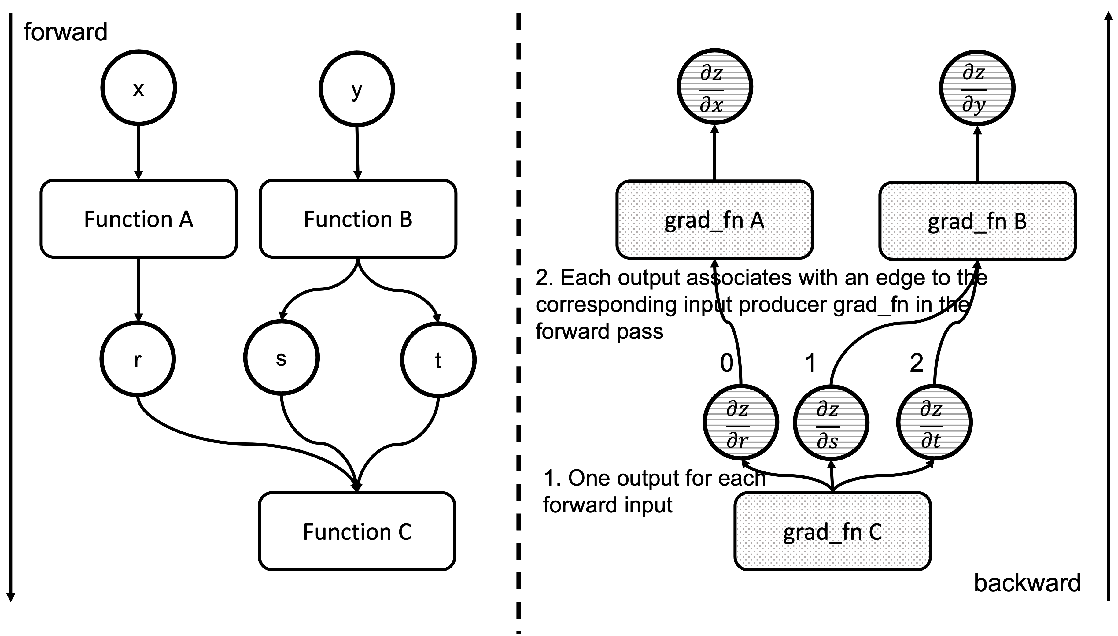
Figure 4: Correspondence between forward and backward functions inputs and outputs

We now iterate through these edges and check if the associated functions are ready to be executed.

 // Check if the next function is ready to be computed
    bool is_ready = false;
    auto& dependencies = graph_task->dependencies_;
    auto it = dependencies.find(next.function.get());

    if (it == dependencies.end()) {
      auto name = next.function->name();
      throw std::runtime_error(std::string("dependency not found for ") + name);
    } else if (--it->second == 0) {
      dependencies.erase(it);
      is_ready = true;
    }

    auto& not_ready = graph_task->not_ready_;
    auto not_ready_it = not_ready.find(next.function.get());

For this, we check the graph_task->dependencies_ map. We decrement the counter, and if it reaches 0, we mark the function pointed by the edge ready to be executed. Following, we prepare the input buffers of the tasks indicated by the next edges.

    if (not_ready_it == not_ready.end()) {
      if (!exec_info_.empty()) {
        // Skip functions that aren't supposed to be executed
      }

      // Creates an InputBuffer and moves the output to the corresponding input position
      InputBuffer input_buffer(next.function->num_inputs());
      input_buffer.add(next.input_nr,
                       std::move(output),
                       opt_parent_stream,
                       opt_next_stream);

      if (is_ready) {
        auto queue = ready_queue(cpu_ready_queue, input_buffer.device());
        queue->push(
            NodeTask(graph_task, next.function, std::move(input_buffer)));
      } else {
        not_ready.emplace(next.function.get(), std::move(input_buffer));
      }

Here, we look for the task in the graph_task->not_ready_ map. If it is not present, we create a new InputBuffer object and set the current output in the input_nr position of the buffer associated with the edge. If the task is ready to be executed, we enqueue it in the appropriate device ready_queue and complete the execution. However, if the task is not ready and we have seen it before, it is present in the not_ready_map_.

    } else {
      // The function already has a buffer
      auto &input_buffer = not_ready_it->second;
      // Accumulates into buffer
      input_buffer.add(next.input_nr,
                       std::move(output),
                       opt_parent_stream,
                       opt_next_stream);
      if (is_ready) {
        auto queue = ready_queue(cpu_ready_queue, input_buffer.device());
        queue->push(NodeTask(graph_task, next.function, std::move(input_buffer)));
        not_ready.erase(not_ready_it);
      }
    }
  }
}

In this case, we accumulate the output in the existing input_buffer instead of creating a new one. Once all the tasks are processed, the worker thread exits the loop and complete.
All this process is summarized in the animation in Figure 5. We see how a thread peeks at the tasks in the ready queue and decrements the next nodes’ dependencies, unlocking them for execution.

Figure 5: Animation of the execution of the computational graph

Flow with Reentrant Backward

As we saw above, the reentrant backward problem is when the currently executed function does a nested call to backward. When this happens, the thread running this function goes all the way down to execute_with_graph_task as in the non-reentrant case, but here is when things are different.

c10::intrusive_ptr<at::ivalue::Future> Engine::execute_with_graph_task(
    const std::shared_ptr<GraphTask>& graph_task,
    std::shared_ptr<Node> graph_root,
    InputBuffer&& input_buffer) {

  initialize_device_threads_pool();
  // Lock mutex for GraphTask.
  std::unique_lock<std::mutex> lock(graph_task->mutex_);

  auto queue = ready_queue(graph_task->cpu_ready_queue_, input_buffer.device());

  if (worker_device == NO_DEVICE) {
    //Regular case
  } else {
    // If worker_device is any devices (i.e. CPU, CUDA): this is a re-entrant
    //    backward call from that device.
    graph_task->owner_ = worker_device;

    // Now that all the non-thread safe fields of the graph_task have been populated,
    // we can enqueue it.
    queue->push(NodeTask(graph_task, std::move(graph_root), std::move(input_buffer)));

    if (current_depth >= max_recursion_depth_) {
      // If reached the max depth, switch to a different thread
      add_thread_pool_task(graph_task);
    } else {
      ++total_depth;
      ++current_depth;
      lock.unlock();
      thread_main(graph_task);
      --current_depth;
      --total_depth;
    }
  }
  return graph_task->future_result_;
}

Here, execute_with_graph_task detects this as a reentrant call and then looks for the current number of nested calls. If it exceeds the limit, we create a new thread to take care of the execution of this graph, and if not, we execute this reentrant call regularly.
The limit of nested calls was originally set to avoid stack overflow due to reentrant calls creating very large call stacks. However, the number was further reduced when sanitizer tests were added because of the maximum amount of locks a thread can hold at a given moment. This can be seen in torch/csrc/autograd/engine.h.

When this maximum depth is exceeded, a new thread is created with the add_thread_pool_task function.

void Engine::add_thread_pool_task(const std::weak_ptr<GraphTask>& graph_task) {
  std::unique_lock<std::mutex> lck(thread_pool_shared_->mutex_);
  // if we have pending graph_task objects to be processed, create a worker.
   bool create_thread = (thread_pool_shared_->num_workers_ <= thread_pool_shared_->graphtasks_queue_.size());
  thread_pool_shared_->graphtasks_queue_.push(graph_task);


  lck.unlock();
  if (create_thread) {
    std::thread t(&Engine::reentrant_thread_init, this);
    t.detach();
  }

  thread_pool_shared_->work_.notify_one();
}


Before going in-depth, let’s look at the thread_pool_shared_ object in the Engine which manages all the information related to the threads associated to the reentrant backward calls.

  struct ThreadPoolShared {
    unsigned int num_workers_;
    std::condition_variable work_;
    std::mutex mutex_;
    std::queue<std::weak_ptr<GraphTask>> graphtasks_queue_;

    // NOLINTNEXTLINE(cppcoreguidelines-pro-type-member-init)
    ThreadPoolShared() : num_workers_(0) {}
 };


ThreadPoolShared is a simple container holding a queue of GraphTask objects with synchronization mechanisms and the number of current workers.

Now it is easy to understand how add_thread_pool_task creates a thread when there are graph_task objects enqueued and insufficient workers to process them.

add_thread_pool_task initializes a thread by executing reentrant_thread_init

void Engine::reentrant_thread_init() {
  at::init_num_threads();
  auto tp_shared = thread_pool_shared_;
  while(true) {
    std::unique_lock<std::mutex> lk(tp_shared->mutex_);
    ++thread_pool_shared_->num_workers_;
    tp_shared->work_.wait(lk, [&tp_shared]{ return !tp_shared->graphtasks_queue_.empty();});
    --thread_pool_shared_->num_workers_;
    auto task = tp_shared->graphtasks_queue_.front();
    tp_shared->graphtasks_queue_.pop();
    lk.unlock();
    std::shared_ptr<GraphTask> graph_task;
    if (!(graph_task = task.lock())) {
      continue;
    }
    set_device(graph_task->owner_);
    // set the local_ready_queue to the ready queue on the graph_task->owner_ device
    local_ready_queue = ready_queue_by_index(graph_task->cpu_ready_queue_, graph_task->owner_);
    total_depth = graph_task->reentrant_depth_;
    thread_main(graph_task);
  }
}


The code is straightforward. The newly created thread waits on the thread_pool_shared->graphtasks_queue_ for reentrant backward graphs to be available and executes them. Notice that this thread uses the task-ready queue associated with the device of the thread that started this call by accessing the graph_task->owner_ field set in the execute_with_graph_task function.

Error Handling

Whenever an error happens in one of the worker threads. It will be propagated to the backward calling thread.

To achieve this, there is a try/catch block in the thread_main that catches any exception in the Node function call and sets it to the associated GraphTask object.

       try {
          
          GraphTaskGuard guard(local_graph_task);
          NodeGuard ndguard(task.fn_);
          {
            evaluate_function(
               
          }
        } catch (std::exception& e) {
          thread_on_exception(local_graph_task, task.fn_, e);
        }
      }
    }

thread_on_exception and the functions it calls end up setting the exception in the local_graph_task object.

void Engine::thread_on_exception(
    std::shared_ptr<GraphTask> graph_task,
    const std::shared_ptr<Node>& fn,
    std::exception& e) {
  graph_task->set_exception(std::current_exception(), fn);
}

void GraphTask::set_exception_without_signal(const std::shared_ptr<Node>& fn) {
  if (!has_error_.exchange(true)) {
    if (AnomalyMode::is_enabled() && fn) {
      fn->metadata()->print_stack(fn->name());
    }
  }
}

void GraphTask::set_exception(
    std::exception_ptr eptr,
    const std::shared_ptr<Node>& fn) {
  set_exception_without_signal(fn);
  if (!future_completed_.exchange(true)) {
    // NOLINTNEXTLINE(performance-move-const-arg)
    future_result_->setError(std::move(eptr));
  }
}

In set_exception it sets the has_error_ flag to true and it calls the setError
function of the future_result_ object. This will make the error to be re-thrown at the caller thread when future_result_->value() is accessed.

 IValue value() {
    std::unique_lock<std::mutex> lock(mutex_);
    AT_ASSERT(completed());
    if (eptr_) {
      std::rethrow_exception(eptr_);
    }
    return value_;
  }

Closing Remarks

This has been the last post of this series covering how PyTorch does the auto differentiation. We hope you enjoyed reading it and that now you are familiar enough with PyTorch internals to start contributing in PyTorch development!

Read More

Choose specific timeseries to forecast with Amazon Forecast

Today, we’re excited to announce that Amazon Forecast offers the ability to generate forecasts on a selected subset of items. This helps you to leverage the full value of your data, and apply it selectively on your choice of items reducing the time and effort to get forecasted results.

Generating a forecast on ‘all’ items of the dataset restricted you from the freedom to have fine-grained controls over specific items that you wanted to forecast. This meant increased cost for low/no priority forecasted items and additional overhead. Earlier, you would spend a lot of time generating multiple predictions on all of the items in your data. This was time consuming and operationally heavy to manage. Moreover, this approach doesn’t fully leverage the value of machine learning (ML): applying inferences across desired items. With the capability to choose a subset of items, you can now focus on training the model with all of your data, but apply the learnings to select few high yield items. This will contribute to overall optimization of forecast planning by increasing productivity (fewer items to manage) and reducing cost (reduction in price per forecasted item). This also makes explainability easier to manage.

With today’s launch, you can not only run all of the steps, but also have the choice to select a subset of items to forecast by uploading a csv during the ‘Create a Forecast’ step. You don’t need to onboard the entire target or related timeseries and item metadata which saves considerable effort for you. This will also help when reducing the overall infrastructure footprint for forecasted items resulting in cost savings and productivity. You can do this step using the ‘CreateForecast’ API, or follow the following console steps.

Forecast on select subset of items

Now we will walk through how to use the Forecast console to choose select items on the input dataset.

Step 1: Import Training Data

To import time-series data into Forecast, create a dataset group, choose a domain for your dataset group, specify the details of your data, and point Forecast to the Amazon Simple Storage Service (Amazon S3) location of your data. In this example, let’s assume that your dataset has 1000 items.

Note: This exercise assumes that you haven’t created any dataset groups. If you previously created a dataset group, then what you see will vary slightly from the following screenshots and instructions.

To import time-series data for forecasting

  1. Open the Forecast console here.
  2. On the Forecast home page, choose Create dataset group.
  3. On the Create dataset group page, add the details for your input dataset.
  4. Choose Next.
  5. The Dataset details panel should look similar to the following:
  6. After you’ve entered all of the necessary details on the dataset import page, the Dataset import details panel should look similar to the following:
  7. Choose Start.

Wait for Forecast to finish importing your time series data. The process can take several minutes or longer. When your dataset has been imported, the status transitions to Active and the banner at the top of the dashboard notifies you that you have successfully imported your data.

Now that your target time series dataset has been imported, you can create a predictor.

Step 2: Create a predictor

Next, you create a predictor, which you use to generate forecasts based on your time series data. Forecast applies the optimal combination of algorithms to each time series in your datasets.

To create a predictor with the Forecast console, you specify a predictor name, a forecast frequency, and define a forecast horizon. For more information about the additional fields that you can configure, see Training Predictors.

To create a predictor

  1. After your target time series dataset has finished importing, your dataset group’s Dashboard should look similar to the following:

    Under Train a predictor, choose Start. The Train predictor page is displayed.
  2. On the Train predictor page, for Predictor settings, provide the following information:
    • Predictor name
    • Forecast frequency
    • Forecast horizon
    • Forecast dimensions and Forecast quantiles (optional)

Now that your predictor has been trained on 1000 items, you can head to the next step of generating a Forecast.

Step 3: Create a Forecast

  1. Select Create Forecast.
  2. Write the Forecast name
  3. Select a predictor.
  4. Select quantiles – Enter up to five quantiles.
  5. If you want to generate the forecast for all 1000 items, then select “All Items”.
  6. Or else you can select “Selected Items”, which will let you choose specific items out of the 1000 items to forecast.
  7. Provide the location for the s3 file which contains the selected timeseries. Timeseries must include all item and dimension columns specified in the target time series.
  8. You must also define your schema for the input file containing the selected timeseries. The order of columns defined in the schema should match the order of columns in the input file.
  9. Hit Generate Forecast.
  10. Perform an export and the .csv file will show you only the selected items that you chose.

Conclusion

Forecast now provides you with the ability to select a subset of items from the input dataset. With this feature, you can train your model with all of the data available and then apply the learnings to select items that you want to forecast. This helps in saving time and focusing efforts on high priority items. You can achieve cost reduction and better align efforts to business outcomes. “Forecast select items” is available in all Regions where Forecast is publicly available.

To learn more about the forecasting of “selected items”, visit this notebook or read more on the Forecast developer guide.


About the Authors

Meetish Dave is a Sr Product Manager in the Amazon Forecast team. He is interested in all things data and application of those to generate new revenue streams. Outside work, he likes to cook Indian food and watch interesting shows.

Ridhim Rastogi is a Software Development Engineer in the Amazon Forecast team. He is passionate about building scalable distributed systems with a focus on solving real world problems through AI/ML. In his spare time, he likes to solve puzzles, read fiction and explore.

Read More

Improve ML developer productivity with Weights & Biases: A computer vision example on Amazon SageMaker

The content and opinions in this post are those of the third-party author and AWS is not responsible for the content or accuracy of this post.

As more organizations use deep learning techniques such as computer vision and natural language processing, the machine learning (ML) developer persona needs scalable tooling around experiment tracking, lineage, and collaboration. Experiment tracking includes metadata such as operating system, infrastructure used, library, and input and output datasets—often tracked on a spreadsheet manually. Lineage involves tracking the datasets, transformations, and algorithms used to create an ML model. Collaboration includes ML developers working on a single project and also ML developers sharing their results across teams and to business stakeholders—a process commonly done via email, screenshots, and PowerPoint presentations.

In this post, we train a model to identify objects for an autonomous vehicle use case using Weights & Biases (W&B) and Amazon SageMaker. We showcase how the joint solution reduces manual work for the ML developer, creates more transparency in the model development process, and enables teams to collaborate on projects.

We run this example on Amazon SageMaker Studio for you to try out for yourself.

Overview of Weights & Biases

Weights & Biases helps ML teams build better models faster. With just a few lines of code in your SageMaker notebook, you can instantly debug, compare, and reproduce your models—architecture, hyperparameters, git commits, model weights, GPU usage, datasets, and predictions—all while collaborating with your teammates.

W&B is trusted by more than 200,000 ML practitioners from some of the most innovative companies and research organizations in the world. To try it for free, sign up at Weights & Biases, or visit the W&B AWS Marketplace listing.

Getting started with SageMaker Studio

SageMaker Studio is the first fully integrated development environment (IDE) for ML. Studio provides a single web-based interface where ML practitioners and data scientists can build, train, and deploy models with a few clicks, all in one place.

To get started with Studio, you need an AWS account and an AWS Identity and Access Management (IAM) user or role with permissions to create a Studio domain. Refer to Onboard to Amazon SageMaker Domain to create a domain, and the Studio documentation for an overview on using Studio visual interface and notebooks.

Set up the environment

For this post, we’re interested in running our own code, so let’s import some notebooks from GitHub. We use the following GitHub repo as an example, so let’s load this notebook.

You can clone a repository either through the terminal or the Studio UI. To clone a repository through the terminal, open a system terminal (on the File menu, choose New and Terminal) and enter the following command:

git clone https://github.com/wandb/SageMakerStudioLab

To clone a repository from the Studio UI, see Clone a Git Repository in SageMaker Studio.

To get started, choose the 01_data_processing.ipynb notebook. You’re prompted with a kernel switcher prompt. This example uses PyTorch, so we can choose the pre-built PyTorch 1.10 Python 3.8 GPU optimized image to start our notebook. You can see the app starting, and when the kernel is ready, it shows the instance type and kernel on the top right of your notebook.

Our notebook needs some additional dependencies. This repository provides a requirements.txt with the additional dependencies. Run the first cell to install the required dependencies:

%pip install -r requirements.txt

You can also create a lifecycle configuration to automatically install the packages every time you start the PyTorch app. See Customize Amazon SageMaker Studio using Lifecycle Configurations for instructions and a sample implementation.

Use Weights & Biases in SageMaker Studio

Weights & Biases (wandb) is a standard Python library. Once installed, it’s as simple as adding a few lines of code to your training script and you’re ready to log experiments. We have already installed it through our requirements.txt file. You can also install it manually with the following code:

! pip install wandb

Case study: Autonomous vehicle semantic segmentation

Dataset

We use the Cambridge-driving Labeled Video Database (CamVid) for this example. It contains a collection of videos with object class semantic labels, complete with metadata. The database provides ground truth labels that associate each pixel with one of 32 semantic classes. We can version our dataset as a wandb.Artifact, that way we can reference it later. See the following code:

with wandb.init(project="sagemaker_camvid_demo", job_type="upload"):
   artifact = wandb.Artifact(
       name='camvid-dataset',
       type='dataset',
       metadata={
           "url": 'https://s3.amazonaws.com/fast-ai-imagelocal/camvid.tgz',
           "class_labels": class_labels
       },
       description="The Cambridge-driving Labeled Video Database (CamVid) is the first collection of videos with object class semantic labels, complete with metadata. The database provides ground truth labels that associate each pixel with one of 32 semantic classes."
   )
   artifact.add_dir(path)
   wandb.log_artifact(artifact)

You can follow along in the 01_data_processing.ipynb notebook.

We also log a table of the dataset. Tables are rich and powerful DataFrame-like entities that enable you to query and analyze tabular data. You can understand your datasets, visualize model predictions, and share insights in a central dashboard.

Weights & Biases tables support many rich media formats, like image, audio, and waveforms. For a full list of media formats, refer to Data Types.

The following screenshot shows a table with raw images with the ground truth segmentations. You can also view an interactive version of this table.

Train a model

We can now create a model and train it on our dataset. We use PyTorch and fastai to quickly prototype a baseline and then use wandb.Sweeps to optimize our hyperparameters. Follow along in the 02_semantic_segmentation.ipynb notebook. When prompted for a kernel on opening the notebook, choose the same kernel from our first notebook, PyTorch 1.10 Python 3.8 GPU optimized. Your packages are already installed because you’re using the same app.

The model is supposed to learn a per-pixel annotation of a scene captured from the point of view of the autonomous agent. The model needs to categorize or segment each pixel of a given scene into 32 relevant categories, such as road, pedestrian, sidewalk, or cars. You can choose any of the segmented images on the table and access this interactive interface for accessing the segmentation results and categories.

Because the fastai library has integration with wandb, you can simply pass the WandbCallback to the Learner:

from fastai.callback.wandb import WandbCallback

loss_func=FocalLossFlat(axis=1)
model = SegmentationModel(backbone, hidden_dim, num_classes=num_classes)
wandb_callback = WandbCallback(log_preds=True)
   learner = Learner(
        data_loader,
        model,
        loss_func=loss_func,
        metrics=metrics,
        cbs=[wandb_callback],
    )

learn.fit_one_cycle(TRAIN_EPOCHS, LEARNING_RATE)

For the baseline experiments, we decided to use a simple architecture inspired by the UNet paper with different backbones from timm. We trained our models with Focal Loss as criterion. With Weights & Biases, you can easily create dashboards with summaries of your experiments to quickly analyze training results, as shown in the following screenshot. You can also view this dashboard interactively.

Hyperparameter search with sweeps

To improve the performance of the baseline model, we need to select the best model and the best set of hyperparameters to train. W&B makes this easy for us using sweeps.

We perform a Bayesian hyperparameter search with the goal of maximizing the foreground accuracy of the model on the validation dataset. To perform the sweep, we define the configuration file sweep.yaml. Inside this file, we pass the desired method to use: bayes and the parameters and their corresponding values to search. In our case, we try different backbones, batch sizes, and loss functions. We also explore different optimization parameters like learning rate and weight decay. Because these are continuous values, we sample from a distribution. There are multiple configuration options available for sweeps.

program: train.py
project: sagemaker_camvid_demo
method: bayes
metric:
    name: foreground_acc
    goal: maximize
early_terminate:
    type: hyperband
    min_iter: 5
parameters:
    backbone:
        values: ["mobilenetv2_100","mobilenetv3_small_050","mobilenetv3_large_100","resnet18","resnet34","resnet50","vgg19"]
    batch_size: 
        values: [8, 16]
    image_resize_factor: 
        value: 4
    loss_function: 
        values: ["categorical_cross_entropy", "focal", "dice"]
    learning_rate: 
        distribution: uniform 
        min: 1e-5
        max: 1e-2
    weight_decay: 
        distribution: uniform
        min: 0.0 
        max: 0.05

Afterwards, in a terminal, you launch the sweep using the wandb command line:

$ wandb sweep sweep.yaml —-project="sagemaker_camvid_demo"

And then launch a sweep agent on this machine with the following code:

$ wandb agent <sweep_id>

When the sweep has finished, we can use a parallel coordinates plot to explore the performances of the models with various backbones and different sets of hyperparameters. Based on that, we can see which model performs the best.

The following screenshot shows the results of the sweeps, including a parallel coordinates chart and parameter correlation charts. You can also view this sweeps dashboard interactively.

We can derive the following key insights from the sweep:

  • Lower learning rate and lower weight decay results in better foreground accuracy and Dice scores.
  • Batch size has strong positive correlations with the metrics.
  • The VGG-based backbones might not be a good option to train our final model because they’re prone to resulting in a vanishing gradient. (They’re filtered out as the loss diverged.)
  • The ResNet backbones result in the best overall performance with respect to the metrics.
  • The ResNet34 or ResNet50 backbone should be chosen for the final model due to their strong performance in terms of metrics.

Data and model lineage

W&B artifacts were designed to make it effortless to version your datasets and models, regardless of whether you want to store your files with W&B or whether you already have a bucket you want W&B to track. After you track your datasets or model files, W&B automatically logs each modification, giving you a complete and auditable history of changes to your files.

In our case, the dataset, models, and different tables generated during training are logged to the workspace. You can quickly view and visualize this lineage by going to the Artifacts page.

Interpret model predictions

Weight & Biases is especially useful when assessing model performance by using the power of wandb.Tables to visualize where our model is doing badly. In this case, we’re particularly interested in detecting correctly vulnerable users like bicycles and pedestrians.

We logged the predicted masks along with the per-class Dice score coefficient into a table. We then filtered by rows containing the desired classes and sorted by ascending order on the Dice score.

In the following table, we first filter by choosing where the Dice score is positive (pedestrians are present in the image). Then we sort in ascending order to identify our worst-detected pedestrians. Keep in mind that a Dice score equaling 1 means correctly segmenting the pedestrian class. You can also view this table interactively.

We can repeat this analysis with other vulnerable classes, such as bicycles or traffic lights.

This feature is a very good way of identifying images that aren’t labeled correctly and tagging them to re-annotate.

Conclusion

This post showcased the Weights & Biases MLOps platform, how to set up W&B in SageMaker Studio, and how to run an introductory notebook on the joint solution. We then ran through an autonomous vehicle semantic segmentation use case and demonstrated tracking training runs with W&B experiments, hyperparameter optimization using W&B sweeps, and interpreting results with W&B tables.

If you’re interested in learning more, you can access the live W&B report. To try Weights & Biases for free, sign up at Weights & Biases, or visit the W&B AWS Marketplace listing.


About the Authors

Thomas Capelle is a Machine Learning Engineer at Weights and Biases. He is responsible for keeping the www.github.com/wandb/examples repository live and up to date. He also builds content on MLOPS, applications of W&B to industries, and fun deep learning in general. Previously he was using deep learning to solve short-term forecasting for solar energy. He has a background in Urban Planning, Combinatorial Optimization, Transportation Economics, and Applied Math.

Durga Sury is a ML Solutions Architect in the Amazon SageMaker Service SA team. She is passionate about making machine learning accessible to everyone. In her 3 years at AWS, she has helped set up AI/ML platforms for enterprise customers. When she isn’t working, she loves motorcycle rides, mystery novels, and hikes with her four-year old husky.

Karthik Bharathy is the product leader for Amazon SageMaker with over a decade of product management, product strategy, execution and launch experience.

Read More

How Cepsa used Amazon SageMaker and AWS Step Functions to industrialize their ML projects and operate their models at scale

This blog post is co-authored by Guillermo Ribeiro, Sr. Data Scientist at Cepsa.

Machine learning (ML) has rapidly evolved from being a fashionable trend emerging from academic environments and innovation departments to becoming a key means to deliver value across businesses in every industry. This transition from experiments in laboratories to solving real-world problems in production environments goes hand in hand with MLOps, or the adaptation of DevOps to the ML world.

MLOps helps streamline and automate the full lifecycle of an ML model, putting its focus on the source datasets, experiment reproducibility, ML algorithm code, and model quality.

At Cepsa, a global energy company, we use ML to tackle complex problems across our lines of businesses, from doing predictive maintenance for industrial equipment to monitoring and improving petrochemical processes at our refineries.

In this post, we discuss how we built our reference architecture for MLOps using the following key AWS services:

  • Amazon SageMaker, a service to build, train, and deploy ML models
  • AWS Step Functions, a serverless low-code visual workflow service used to orchestrate and automate processes
  • Amazon EventBridge, a serverless event bus
  • AWS Lambda, a serverless compute service that allows you to run code without provisioning or managing servers

We also explain how we applied this reference architecture to bootstrap new ML projects in our company.

The challenge

During the last 4 years, multiple lines of business across Cepsa kicked off ML projects, but soon certain issues and limitations started to arise.

We didn’t have a reference architecture for ML, so each project followed a different implementation path, performing ad hoc model training and deployment. Without a common method to handle project code and parameters and without an ML model registry or versioning system, we lost the traceability amongst datasets, code, and models.

We also detected room for improvement in the way we operated models in production, because we didn’t monitor deployed models and therefore didn’t have the means to track model performance. As a consequence, we usually retrained models based on time schedules, because we lacked the right metrics to make informed retraining decisions.

The solution

Starting from the challenges we had to overcome, we designed a general solution that aimed to decouple data preparation, model training, inference, and model monitoring, and featured a centralized model registry. This way, we simplified managing environments across multiple AWS accounts, while introducing centralized model traceability.

Our data scientists and developers use AWS Cloud9 (a cloud IDE for writing, running, and debugging code) for data wrangling and ML experimentation and GitHub as the Git code repository.

An automatic training workflow uses the code built by the data science team to train models on SageMaker and to register output models in the model registry.

A different workflow manages model deployment: it obtains the reference from the model registry and creates an inference endpoint using SageMaker model hosting features.

We implemented both model training and deployment workflows using Step Functions, because it provided a flexible framework that enables the creation of specific workflows for each project and orchestrates different AWS services and components in a straightforward way.

Data consumption model

In Cepsa, we use a series of data lakes to cover diverse business needs, and all these data lakes share a common data consumption model that makes it easier for data engineers and data scientists to find and consume the data they need.

To easily handle costs and responsibilities, data lake environments are completely separated from data producer and consumer applications, and deployed in different AWS accounts belonging to a common AWS Organization.

The data used to train ML models and the data used as an inference input for trained models is made available from the different data lakes through a set of well-defined APIs using Amazon API Gateway, a service to create, publish, maintain, monitor, and secure APIs at scale. The API backend uses Amazon Athena (an interactive query service to analyze data using standard SQL) to access data that is already stored in Amazon Simple Storage Service (Amazon S3) and cataloged in the AWS Glue Data Catalog.

The following diagram provides a general overview of Cepsa’s MLOps architecture.

Model training

The training process is independent for each model and handled by a Step Functions standard workflow, which gives us flexibility to model processes based on different project requirements. We have a defined a base template that we reuse on most projects, performing minor adjustments when required. For example, some project owners have decided to add manual gates to approve deployments of new production models, while other project owners have implemented their own error detection and retry mechanisms.

We also perform transformations on the input datasets used for model training. For this purpose, we use Lambda functions that are integrated in the training workflows. In some scenarios where more complex data transformations are required, we run our code in Amazon Elastic Container Service (Amazon ECS) on AWS Fargate, a serverless compute engine to run containers.

Our data science team uses custom algorithms frequently, so we take advantage of the ability to use custom containers in SageMaker model training, relying on Amazon Elastic Container Registry (Amazon ECR), a fully managed container registry that makes it easy to store, manage, share, and deploy container images.

Most of our ML projects are based on the Scikit-learn library, so we have extended the standard SageMaker Scikit-learn container to include the environment variables required for the project, such as the Git repository information and deployment options.

With this approach, our data scientists just need to focus on developing the training algorithm and to specify the libraries required by the project. When they push code changes to the Git repository, our CI/CD system (Jenkins hosted on AWS) builds the container with the training code and libraries. This container is pushed to Amazon ECR and finally passed as a parameter to the SageMaker training invocation.

When the training process is complete, the resulting model is stored in Amazon S3, a reference is added in the model registry, and all the collected information and metrics are saved in the experiments catalog. This assures full reproducibility because the algorithm code and libraries are linked to the trained model along with the data associated to the experiment.

The following diagram illustrates the model training and retraining process.

Model deployment

The architecture is flexible and allows both automatic and manual deployments of the trained models. The model deployer workflow is automatically invoked by means of an event that SageMaker training publishes in EventBridge after training has finished, but it can also be manually invoked if needed, passing the right model version from the model registry. For more information about automatic invocation, see Automating Amazon SageMaker with Amazon EventBridge.

The model deployer workflow retrieves the model information from the model registry and uses AWS CloudFormation, a managed infrastructure as code service, to either deploy the model to a real-time inference endpoint or perform batch inference with a stored input dataset, depending on the project requirements.

Whenever a model is successfully deployed in any environment, the model registry is updated with a new tag indicating on which environments the model is currently running. Any time an endpoint is removed, its tag is also deleted from the model registry.

The following diagram shows the workflow for model deployment and inference.

Experiments and model registry

Storing every experiment and model version in a single location and having a centralized code repository enables us to decouple model training and deployment and to use different AWS accounts for every project and environment.

All experiment entries store the commit ID of the training and inference code, so we have complete traceability of the whole experimentation process and are able to easily compare different experiments. This prevents us from performing duplicate work on the scientific exploration phase for algorithms and models, and enables us to deploy our models anywhere, independently from the account and environment where the model was trained. This also holds true for models trained in our AWS Cloud9 experimentation environment.

All in all, we have fully automated model training and deployment pipelines and have the flexibility to perform fast manual model deployments when something isn’t working properly or when a team needs a model deployed to a different environment for experimentation purposes.

A detailed use case: YET Dragon project

The YET Dragon project aims to improve the production performance of Cepsa’s petrochemical plant in Shanghai. To achieve this goal, we studied the production process thoroughly, looking for the less efficient steps. Our target was to increase the yield efficiency of the processes by keeping component concentration exactly below a threshold.

To simulate this process, we built four generalized additive models or GAM, linear models whose response depends on smooth functions of predictor variables, to predict the results of two oxidation processes, one concentration process, and the aforementioned yield. We also built an optimizer to process the results of the four GAM models and find the best optimizations that could be applied in the plant.

Although our models are trained with historical data, the plant can sometimes operate under circumstances that weren’t registered in the training dataset; we expect that our simulation models won’t work well under those scenarios so we also built two anomaly detection models using Isolation Forests algorithms, which determine how far are data points to the rest of the data to detect the anomalies. These models help us detect such situations to disable the automated optimization processes whenever this happens.

Industrial chemical processes are highly variable and the ML models need to be well aligned with the plant operation, so frequent retraining is required as well as traceability of the models deployed in each situation. YET Dragon was our first ML optimization project to feature a model registry, full reproducibility of the experiments, and a fully managed automated training process.

Now, the complete pipeline that brings a model into production (data transformation, model training, experiment tracking, model registry, and model deployment) is independent for each ML model. This enables us to improve models iteratively (for example adding new variables or testing new algorithms) and to connect the training and deployment stages to different triggers.

The results and future improvements

We are currently able to automatically train, deploy, and track the six ML models used in the YET Dragon project, and we have already deployed over 30 versions for each of the production models. This MLOps architecture has been extended to hundreds of ML models in other projects across the company.

We plan to keep launching new YET projects based on this architecture, which has decreased project mean duration by 25%, thanks to the reduction of bootstrapping time and the automation of ML pipelines. We have also estimated savings of around €300,000 per year thanks to the increase in yield and concentration that is a direct result of the YET Dragon project.

The short-term evolution of this MLOps architecture is towards model monitoring and automated testing. We plan to automatically test model efficiency against previously deployed models before a new model is deployed. We’re also working in the implementation of model monitoring and inference data drift monitoring with Amazon SageMaker Model Monitor, in order to automate model retraining.

Conclusion

Companies are facing the challenge of bringing their ML projects to production in an automated and efficient manner. Automating the full ML model lifecycle helps reduce project times and ensures better model quality and faster and more frequent deployments to production.

By developing a standardized MLOps architecture that has been adopted by different business across the company, we at Cepsa were able to speed up ML project bootstrapping and to improve ML model quality, providing a reliable and automated framework upon which our data science teams can innovate faster.

For more information about MLOps on SageMaker, visit Amazon SageMaker for MLOps and check out other customer use cases in the AWS Machine Learning Blog.


About the authors

Guillermo Ribeiro Jiménez is a Sr Data Scientist at Cepsa with a PhD. in Nuclear Physics. He has 6 years of experience with data science projects, mainly in the telco and energy industry. He is currently leading data scientist teams in Cepsa’s Digital Transformation department, with a focus on the scaling and productization of machine learning projects.

Guillermo Menéndez Corral is a Solutions Architect at AWS Energy and Utilities. He has over 15 years of experience designing and building SW applications, and currently provides architectural guidance to AWS customers in the energy industry, with a focus on analytics and machine learning.

Read More

Analyze and tag assets stored in Veeva Vault PromoMats using Amazon AppFlow and Amazon AI Services

In a previous post, we talked about analyzing and tagging assets stored in Veeva Vault PromoMats using Amazon AI services and the Veeva Vault Platform’s APIs. In this post, we explore how to use Amazon AppFlow, a fully managed integration service that enables you to securely transfer data from software as a service (SaaS) applications like Veeva Vault to AWS. The Amazon AppFlow Veeva connector allows you to connect your AWS environment to the Veeva ecosystem quickly, reliably, and cost-effectively in order to analyze the rich content stored in Veeva Vault at scale.

The Amazon AppFlow Veeva connector is the first Amazon AppFlow connector supporting automatic transfer of Veeva documents. It allows you to choose between the latest version (the Steady State version in Veeva terms) and all versions of documents. Moreover, you can import document metadata.

With a few clicks, you can easily set up a managed connection and choose the Veeva Vault documents and metadata to import. You can further adjust the import behavior by mapping source fields to destination fields. You can also add filters based on document type and subtype, classification, products, country, site, and more. Lastly, you can add validation and manage on-demand and scheduled flow triggers.

You can use the Amazon AppFlow Veeva connector for various use cases, ranging from Veeva Vault PromoMats to other Veeva Vault solutions such as QualityDocs, eTMF, or Regulatory Information Management (RIM). The following are some of the use cases where you can use the connector:

  • Data synchronization – You can use the connector in the process of establishing consistency and harmonization between data from a source Veeva Vault and any downstream systems over time. For example, you can share Veeva PromoMats marketing assets to Salesforce. You could also use the connector to share Veeva QualityDocs like Standard Operating Procedures (SOPs) or specifications to cached websites that are searchable from tablets present on the manufacturing floor.
  • Anomaly detection – You can share Veeva PromoMats documents to Amazon Lookout for Metrics for anomaly detection. You can also use the connector with Vault RIM in artwork, commercial labels, templates, or patient leaflets before importing them for printing into enterprise labeling solutions such as Loftware.
  • Data lake hydration – The connector can be an effective tool for replicating structured or unstructured data into data lakes, in order to support the creation and hydration of data lakes. For example, you can use the connector to extract standardized study information from protocols stored in Vault RIM and expose it downstream to medical analytics insight teams.
  • Translations – The connector can be useful in sending artwork, clinical documents, marketing materials, or study protocols for translation in native languages to departments such as packaging, clinical trials, or regulatory submissions.

This post focuses on how you can use Amazon AI services in combination with Amazon AppFlow to analyze content stored in Veeva Vault PromoMats, automatically extract tag information, and ultimately feed this information back into the Veeva Vault system. The post discusses the overall architecture, the steps to deploy a solution and dashboard, and a use case of asset metadata tagging. For more information about the proof of concept code base for this use case, see the GitHub repository.

Solution overview

The following diagram illustrates the updated solution architecture.

Solution architecture

Previously, in order to import assets from Veeva Vault, you had to write your own custom code logic using the Veeva Vault APIs to poll for changes and import the data into Amazon Simple Storage Service (Amazon S3). This could be a manual, time-consuming process, in which you had to account for API limitations, failures, and retries, as well as scalability to accommodate an unlimited amount of assets. The updated solution uses Amazon AppFlow to abstract away the complexity of maintaining a custom Veeva to Amazon S3 data import pipeline.

As mentioned in the introduction, Amazon AppFlow is an easy-to-use, no-code self-service tool that uses point-and-click configurations to move data easily and securely between various SaaS applications and AWS services. AppFlow allows you to pull data (objects and documents) from supported sources and write that data to various supported destinations. The source or destination could be a SaaS application or an AWS service such as Amazon S3, Amazon Redshift, or Lookout for Metrics. In addition to the no-code interface, Amazon AppFlow supports configuration via API, AWS CLI, and AWS CloudFormation interfaces.

A flow in Amazon AppFlow describes how data is to be moved, including source details, destination details, flow trigger conditions (on demand, on event, or scheduled), and data processing tasks such as checkpointing, field validation, or masking. When triggered, Amazon AppFlow runs a flow that fetches the source data (generally through the source application’s public APIs), runs data processing tasks, and transfers processed data to the destination.

In this example, you deploy a preconfigured flow using a CloudFormation template. The following screenshot shows the preconfigured veeva-aws-connector flow that is created automatically by the solution template on the Amazon AppFlow console.

Amazon AppFlow Flow Source Details

The flow uses Veeva as a source and is configured to import Veeva Vault component objects. Both the metadata and source files are necessary in order to keep track of the assets that have been processed and push tags back on the correct corresponding asset in the source system. In this situation, only the latest version is being imported, and renditions aren’t included.

Amazon AppFlow Flow destination details

The flow’s destination also needs to be configured. In the following screenshot, we define a file format and folder structure for the S3 bucket that was created as part of the CloudFormation template.

Amazon AppFlow flow trigger options

Finally, the flow is triggered on demand for demonstration purposes. This can be modified so that the flow runs on a schedule, with a maximum granularity of 1 minute. When triggered on a schedule, the transfer mode changes automatically from a full transfer to an incremental transfer mode. You specify a source timestamp field for tracking the changes. For the tagging use case, we have found that the Last Modified Date setting is the most suitable.

Amazon AppFlow flow trigger on schedule options

Amazon AppFlow is then integrated with Amazon EventBridge to publish events whenever a flow run is complete.

For better resiliency, the AVAIAppFlowListener AWS Lambda function is wired into EventBridge. When an Amazon AppFlow event is triggered, it verifies that the specific flow run has completed successfully, reads the metadata information of all imported assets from that specific flow run, and pushes individual document metadata into an Amazon Simple Queue Service (Amazon SQS) queue. Using Amazon SQS provides a loose coupling between the producer and processor sections of the architecture and also allows you to deploy changes to the processor section without stopping the incoming updates.

A second poller function (AVAIQueuePoller) reads the SQS queue at frequent intervals (every minute) and processes the incoming assets. For an even better reaction time from the Lambda function, you can replace the CloudWatch rule by configuring Amazon SQS as a trigger for the function.

Depending on the incoming message type, the solution uses various AWS AI services to derive insights from your data. Some examples include:

  • Text files – The function uses the DetectEntities operation of Amazon Comprehend Medical, a natural language processing (NLP) service that makes it easy to use ML to extract relevant medical information from unstructured text. This operation detects entities in categories like Anatomy, Medical_Condition, Medication, Protected_Health_Information, and Test_Treatment_Procedure. The resulting output is filtered for Protected_Health_Information, and the remaining information, along with confidence scores, is flattened and inserted into an Amazon DynamoDB table. This information is plotted on the OpenSearch Kibana cluster. In real-world applications, you can also use the Amazon Comprehend Medical ICD-10-CM or RxNorm feature to link the detected information to medical ontologies so downstream healthcare applications can use it for further analysis.
  • Images – The function uses the DetectLabels method of Amazon Rekognition to detect labels in the incoming image. These labels can act as tags to identify the rich information buried in your images, such as information about commercial artwork and clinical labels. If labels like Human or Person are detected with a confidence score of more than 80%, the code uses the DetectFaces method to look for key facial features such as eyes, nose, and mouth to detect faces in the input image. Amazon Rekognition delivers all this information with an associated confidence score, which is flattened and stored in the DynamoDB table.
  • Voice recordings – For audio assets, the code uses the StartTranscriptionJob asynchronous method of Amazon Transcribe to transcribe the incoming audio to text, passing in a unique identifier as the TranscriptionJobName. The code assumes the audio language to be English (US), but you can modify it to tie to the information coming from Veeva Vault. The code calls the GetTranscriptionJob method, passing in the same unique identifier as the TranscriptionJobName in a loop, until the job is complete. Amazon Transcribe delivers the output file on an S3 bucket, which is read by the code and deleted. The code calls the text processing workflow (as discussed earlier) to extract entities from transcribed audio.
  • Scanned documents (PDFs) – A large percentage of life sciences assets are represented in PDFs—these could be anything from scientific journals and research papers to drug labels. Amazon Textract is a service that automatically extracts text and data from scanned documents. The code uses the StartDocumentTextDetection method to start an asynchronous job to detect text in the document. The code uses the JobId returned in the response to call GetDocumentTextDetection in a loop, until the job is complete. The output JSON structure contains lines and words of detected text, along with confidence scores for each element it identifies, so you can make informed decisions about how to use the results. The code processes the JSON structure to recreate the text blurb and calls the text processing workflow to extract entities from the text.

A DynamoDB table stores all the processed data. The solution uses DynamoDB Streams and Lambda triggers (AVAIPopulateES) to populate data into an OpenSearch Kibana cluster. The AVAIPopulateES function runs for every update, insert, and delete operation that happens in the DynamoDB table, and inserts one corresponding record in the OpenSearch index. You can visualize these records using Kibana.

To close the feedback loop, the AVAICustomFieldPopulator Lambda function has been created. It’s triggered by events in the DynamoDB stream of the metadata DynamoDB table. For every DocumentID in the DynamoDB records, the function tries to upsert tag information into a predefined custom field property of the asset with the corresponding ID in Veeva, using the Veeva API. To avoid inserting noise into the custom field, the Lambda function filters any tags that have been identified with a confidence score lower than 0.9. Failed requests are forwarded to a dead-letter queue (DLQ) for manual inspection or automatic retry.

This solution offers a serverless, pay-as-you-go approach to process, tag, and enable comprehensive searches on your digital assets. Additionally, each managed component has high availability built in by automatic deployment across multiple Availability Zones. For Amazon OpenSearch Service (successor to Amazon Elasticsearch Service), you can choose the three-AZ option to provide better availability for your domains.

Prerequisites

For this walkthrough, you should have the following prerequisites:

  • An AWS account with appropriate AWS Identity and Access Management (IAM) permissions to launch the CloudFormation template
  • Appropriate access credentials for a Veeva Vault PromoMats domain (domain URL, user name, and password)
  • A custom content tag defined in Veeva for the digital assets that you want to be tagged (as an example, we created the AutoTags custom content tag)
  • Digital assets in the PromoMats Vault accessible to the preceding credentials

Deploy your solution

You use a CloudFormation stack to deploy the solution. The stack creates all the necessary resources, including:

  • An S3 bucket to store the incoming assets.
  • An Amazon AppFlow flow to automatically import assets into the S3 bucket.
  • An EventBridge rule and Lambda function to react to the events generated by Amazon AppFlow (AVAIAppFlowListener).
  • An SQS FIFO queue to act as a loose coupling between the listener function (AVAIAppFlowListener) and the poller function (AVAIQueuePoller).
  • A DynamoDB table to store the output of Amazon AI services.
  • An Amazon OpenSearch Kibana (ELK) cluster to visualize the analyzed tags.
  • A Lambda function to push back identified tags into Veeva (AVAICustomFieldPopulator), with a corresponding DLQ.
  • Required Lambda functions:
    • AVAIAppFlowListener – Triggered by events pushed by Amazon AppFlow to EventBridge. Used for flow run validation and pushing a message to the SQS queue.
    • AVAIQueuePoller – Triggered every 1 minute. Used for polling the SQS queue, processing the assets using Amazon AI services, and populating the DynamoDB table.
    • AVAIPopulateES – Triggered when there is an update, insert, or delete on the DynamoDB table. Used for capturing changes from DynamoDB and populating the ELK cluster.
    • AVAICustomFieldPopulator – Triggered when there is an update, insert, or delete on the DynamoDB table. Used for feeding back tag information into Veeva.
  • The Amazon CloudWatch Events rules that trigger the AVAIQueuePoller function. These triggers are in the DISABLED state by default.
  • Required IAM roles and policies for interacting with EventBridge and the AI services in a scoped-down manner.

To get started, complete the following steps:

  1. Sign in to the AWS Management Console with an account that has the prerequisite IAM permissions.
  2. Choose Launch Stack and open it on a new tab:
    Launch stack button
  3. On the Create stack page, choose Next.Create stack details
  4. On the Specify stack details page, enter a name for the stack.
  5. Enter values for the parameters.
  6. Choose Next.Stack parameters
  7. On the Configure stack options page, leave everything as the default and choose Next.Stack options
  8. On the Review page, in the Capabilities and transforms section, select the three check boxes.
  9. Choose Create stack.Configure stack capabilities
  10. Wait for the stack to complete. You can examine various events from the stack creation process on the Events tab.
  11. After the stack creation is complete, you can look on the Resources tab to see all the resources the CloudFormation template created.
  12. On the Outputs tab, copy the value of ESDomainAccessPrincipal.

This is the ARN of the IAM role that the AVAIPopulateES function assumes. You use it later to configure access to the Amazon OpenSearch Service domain.

Set up Amazon OpenSearch Service and Kibana

This section walks you through securing your Amazon OpenSearch Service cluster and installing a local proxy to access Kibana securely.

  1. On the Amazon OpenSearch Service console, select the domain that was created by the template.
  2. On the Actions menu, choose Modify access policy.OpenSearch modify access policy
  3. For Domain access policy, choose Custom access policy.OpenSearch custom access policy dialog
  4. In the Access policy will be cleared pop-up window, choose Clear and continue.OpenSearch access policy warning
  5. On the next page, configure the following statements to lock down access to the Amazon OpenSearch Service domain:
    1. Allow IPv4 address – Your IP address.
    2. Allow IAM ARN – The value of ESDomainAccessPrincipal you copied earlier.OpenSearch custom access policy details
  6. Choose Submit.

This creates an access policy that grants access to the AVAIPopulateES function and Kibana access from your IP address. For more information about scoping down your access policy, see Configuring access policies.

  1. Wait for the domain status to show as Active.
  2. On the Amazon EventBridge console, under Events, choose Rules. You can see two rules that the CloudFormation template created.
  3. Select the AVAIQueuePollerSchedule rule and enable it by clicking Enable.Enable poller

In 5–8 minutes, the data should start flowing in and entities are created in the Amazon OpenSearch Service cluster. You can now visualize these entities in Kibana. To do this, you use an open-source proxy called aws-es-kibana. To install the proxy on your computer, enter the following code:

aws-es-kibana your_OpenSearch_domain_endpoint

You can find the domain endpoint on the Outputs tab of the CloudFormation stack under ESDomainEndPoint. You should see the following output:

aws-es-kibana console output

Create visualizations and analyze tagged content

Please refer to the original blogpost.

Clean up

To avoid incurring future charges, delete the resources when not in use. You can easily delete all resources by deleting the associated CloudFormation stack. Note that you need to empty the created S3 buckets of content in order for the deletion of the stack to be successful.

Conclusion

In this post, we demonstrated how you can use Amazon AI services in combination with Amazon AppFlow to extend the functionality of Veeva Vault PromoMats and extract valuable information quickly and easily. The built-in loop back mechanism allows you to update the tags back into Veeva Vault and enable auto-tagging of your assets. This makes it easier for your team to find and locate assets quickly.

Although no ML output is perfect, it can come very close to human performance and help offset a substantial portion of your team’s efforts. You can use this additional capacity towards value-added tasks, while dedicating a small capacity to check the output of the ML solution. This solution can also help optimize costs, achieve tagging consistency, and enable quick discovery of existing assets.

Finally, you can maintain ownership of your data and choose which AWS services can process, store, and host the content. AWS doesn’t access or use your content for any purpose without your consent, and never uses customer data to derive information for marketing or advertising. For more information, see Data Privacy FAQ.

You can also extend the functionality of this solution further with additional enhancements. For example, in addition to the AI and ML services in this post, you can easily add any of your custom ML models built using Amazon SageMaker to the architecture.

If you’re interested in exploring additional use cases for Veeva and AWS, please reach out to your AWS account team.

Veeva Systems has reviewed and approved this content. For additional Veeva Vault-related questions, please contact Veeva support.


About the authors

Mayank Thakkar is Head of AI/ML Business Development, Global Healthcare and Life Sciences at AWS. He has more than 18 years of experience in varied industries like healthcare, life sciences, insurance, and retail, specializing in building serverless, artificial intelligence, and machine learning-based solutions to solve real-world industry problems. At AWS, he works closely with big pharma companies around the world to build cutting-edge solutions and help them along their cloud journey. Apart from work, Mayank, along with his wife, is busy raising two energetic and mischievous boys, Aaryan (6) and Kiaan (4), while trying to keep the house from burning down or getting flooded!

Anamaria Todor is a Senior Solutions Architect based in Copenhagen, Denmark. She saw her first computer when she was 4 years old and never let computer science and engineering go ever since. She has worked in various technical roles from full-stack developer, to data engineer, technical lead, and CTO at various Danish companies. Anamaria has a bachelor’s degree in Applied Engineering and Computer Science, a master’s degree in Computer Science, and over 10 years of hands-on AWS experience. At AWS, she works closely with healthcare and life sciences companies in the enterprise segment. When she’s not working or playing video games, she’s coaching girls and female professionals in understanding and finding their path through technology.

Read More

MLOps foundation roadmap for enterprises with Amazon SageMaker

As enterprise businesses embrace machine learning (ML) across their organizations, manual workflows for building, training, and deploying ML models tend to become bottlenecks to innovation. To overcome this, enterprises needs to shape a clear operating model defining how multiple personas, such as data scientists, data engineers, ML engineers, IT, and business stakeholders, should collaborate and interact; how to separate the concerns, responsibilities, and skills; and how to use AWS services optimally. This combination of ML and operations (MLOps) is helping companies streamline their end-to-end ML lifecycle and boost productivity of data scientists while maintaining high model accuracy and enhancing security and compliance.

ML Ops personas, operations and technology

In this post, you learn about the key phases of building an MLOps foundations, how multiple personas work together on this foundation, and the Amazon SageMaker purpose-built tools and built-in integrations with other AWS services that can accelerate the adoption of ML across an enterprise business.

MLOps maturity model

Building an MLOps foundation that can cover the operations, people, and technology needs of enterprise customers is challenging. Therefore, we define the following maturity model that defines the necessary capabilities of MLOps in four key phases.

MLOps maturity model with 4 stages

  1. Initial phase: During this phase, the data scientists are able to experiment and build, train, and deploy models on AWS using SageMaker services. The suggested development environment is Amazon SageMaker Studio, in which the data scientists are able to experiment and collaborate based on Studio notebooks.
  2. Repeatable phase – With the ability to experiment on AWS, the next step is to create automatic workflows to preprocess data and build and train models (ML pipelines). Data scientists collaborate with ML engineers in a separate environment to build robust and production-ready algorithms and source code, orchestrated using Amazon SageMaker Pipelines. The generated models are stored and benchmarked in the Amazon SageMaker model registry.
  3. Reliable phase – Even though the models have been generated via the ML pipelines, they need to be tested before they get promoted to production. Therefore, in this phase, the automatic testing methodology is introduced, for both the model and triggering infrastructure, in an isolated staging (pre-production) environment that simulates production. After a successful run of the test, the models are deployed to the isolated environment of production. To promote the models among the multiple environments, manual evaluation and approvals are required.
  4. Scalable phase – After the productionization of the first ML solution, scaling of the MLOps foundation to support multiple data science teams to collaborate and productionize tens or hundreds of ML use cases is necessary. In this phase, we introduce the templatization of the solutions, which brings speed to value by reducing the development time of new production solutions from weeks to days. Additionally, we automate the instantiation of secure MLOps environments to enable multiple teams to operate on their data reducing the dependency and overhead to IT.

In the following sections, we show how to build an MLOps foundation based on the preceding maturity model and the following tenets:

  • Flexibility – Data scientists are able to accommodate any framework (such as TensorFlow or PyTorch)
  • Reproducibility – Data scientists are able to recreate or observe past experiments (code, data, and results)
  • Reusability – Data scientists and ML engineers are able to reuse source code and ML pipelines, avoiding inconsistencies and cost
  • Scalability – Data scientists and ML engineers are able to scale resources and services on demand
  • Auditability – Data scientists, IT, and legal departments are able to audit logs, versions, and dependencies of artifacts and data
  • Consistency – Because MLOps consists of multiple environments, the foundation needs to eliminate variance between environments

Initial phase

In the initial phase, the goal is to create a secure experimentation environment where the data scientist receives snapshots of data and experiments using SageMaker notebooks to prove that ML can solve a specific business problem. To achieve this, a Studio environment with tailored access to services via VPC endpoints is recommended. The source code of the reference architecture is available in the examples provided by the SageMaker team on the Secure Data Science With Amazon SageMaker Studio Reference Architecture GitHub repo.

In addition to SageMaker services, data scientists can use other services to process the data, such as Amazon EMR, Amazon Athena, and AWS Glue, with notebooks stored and versioned in AWS CodeCommit repositories (see the following figure).

initial phase of MLOps account structure

Repeatable phase

After the data scientists have proven that ML can solve the business problem and are familiarized with SageMaker experimentation, training, and deployment of models, the next step is to start productionizing the ML solution. The following figure illustrates this architecture.

Repeatable phase account structure

At this stage, separation of concern is necessary. We split the environment into multiple AWS accounts:

  1. Data lake – Stores all the ingested data from on premises (or other systems) to the cloud. Data engineers are able to create extract, transform, and load (ETL) pipelines combining multiple data sources and prepare the necessary datasets for the ML use cases. The data is cataloged via the AWS Glue Data Catalog and shared with other users and accounts via AWS Lake Formation (the data governance layer). In the same account, Amazon SageMaker Feature Store can be hosted, but we don’t cover it this post. For more information, refer to Enable feature reuse across accounts and teams using Amazon SageMaker Feature Store.
  2. Experimentation – Enables data scientists to conduct their research. The only difference is that the origin of the data snapshots is the data lake. Data scientists have access only in specific datasets, which can be anonymized in case of GDPR or other data privacy constraints. Furthermore, the experimentation account may have access to the internet to enable data scientists to use new data science frameworks or third-party open-source libraries. Therefore, the experimentation account is considered as part of the non-production environment.
  3. Development (dev) – The first stage of the production environment. The data scientists move from notebooks to the world of automatic workflows and SageMaker Pipelines. They need to collaborate with ML engineers to abstract their code and ensure coverage of testing, error handling, and code quality. The goal is to develop ML pipelines, which are automatic workflows that preprocess, train, evaluate, and register models to the SageMaker model registry. The deployment of the ML pipelines is driven only via CI/CD pipelines, and the access to the AWS Management Console is restricted. Internet connection is not allowed because the ML pipeline has access to production data in the data lake (read-only).
  4. Tooling (or automation) – Hosts the CodeCommit repositories, AWS CodePipeline CI/CD pipelines, SageMaker model registry, and Amazon ECR to host custom containers. Because the data lake is the single point of truth for the data, the tooling account is for the code, containers, and produced artifacts.

Note that this account naming convention and multi-account strategy may vary depending on your business needs, but this structure is meant to show the recommended levels of isolation. For example, you could rename the development account to the model training or build account.

To achieve automatic deployment, it’s important to understand how to move from notebooks to ML pipelines and standardize the code repositories and data structure, which we discuss in the following sections.

From notebooks to ML pipelines

The goal of the development environment is to restructure, augment, improve, and scale the code in notebooks and move it to the ML pipelines. An ML pipeline is a set of steps that are responsible for preprocessing the data, training or using models, and postprocessing the results. Each step should perform one exactly task (a specific transformation) and be abstract enough (for example, pass column names as input parameters) to enable reusability. The following diagram illustrates an example pipeline.

Sample SageMaker Pipeline

To implement ML pipelines, data scientists (or ML engineers) use SageMaker Pipelines. A SageMaker pipeline is a series of interconnected steps (SageMaker processing jobs, training, HPO) that is defined by a JSON pipeline definition using a Python SDK. This pipeline definition encodes a pipeline using a Directed Acyclic Graph (DAG). This DAG gives information about the requirements for and relationships between each step of your ML pipeline.

Depending on the use case, you can separate the ML pipeline into two main types: training and batch inference.

The following figure illustrates the training ML pipeline flow.

ML Build pipeline

The preprocessing phase might consist of multiple steps. Common data science transformations are data splitting and sampling (train, validation, test set), one-hot encoding or vectorization, binning, and scaling. The model training step could be either one training job, if the data scientist is aware of the best model configuration, or a hyperparameter optimization (HPO) job, in which AWS defines the best hyperparameters for the model (Bayesian method) and produces the corresponding model artifact. In the evaluation step, the produced model artifact is used to perform inference to the validation dataset. Then the ML pipeline checks if the produced accuracy metrics (such as F1, precision, and gain deciles) pass the necessary thresholds. If this step is successful, the model artifacts and metadata are moved to the model registry for productionization. Note that the export baseline step exploits Amazon SageMaker Model Monitor functionality, producing a JSON object with the statistics that are used later for model drifting detection and can be hosted in the SageMaker model registry as model metadata.

In case of batch inference, the data scientists are able to create similar pipelines, as illustrated in the following figure.

ML Inference pipeline

The preprocessing step of batch inference is often the same as training by excluding data sampling and the column of ground truth. Batch inference is the step that sends data in batches for inference to the corresponding endpoint, and can be implemented by using batch transform. The postprocessing step produces additional statistics, such as result distribution, or joins the results with external IDs. Then, a model monitor step is able to compare the baseline statistics of the data used for training (model JSON metadata in the model registry) against the new incoming data for inference.

You can skip the preprocessing steps if the data scientists create pipeline models that can be stored in the SageMaker model registry. For more details, refer to Host models along with pre-processing logic as serial inference pipeline behind one endpoint.

Standardising repositories

To enable the collaboration between data scientists and ML engineers, the standardization of the code repository structure is necessary. In addition, standardization is beneficial for the CI/CD pipeline structure, enabling the incorporation of automatic validation, building (such as custom container building), and testing steps.

The following example illustrates the separation of the ML solutions into two repositories: a building and training repository for training (and optionally pipeline model), and deployment to promote the batch inference pipeline models or instantiate the real-time endpoints:

Building/Training Repository

# Building/Training Repository
algorithms/
    shared_libraries/
        test/
            input/ # (optional)
            output/ # (optional)
            test_<step>.py
        <help_functions1>.py
        <help_functions2>.py
        README.md
    preprocessing/ # 1 folder per pre-processing job, order is defined in the ml pipeline logic
        <preprocessing_job_name1> # e.g classic ml: one hot encoding
            test/
                input/ # (optional)
                output/ # (optional)
                test_<step>.py
            __main__.py
            dockerfile # (optional) define dockerfile in case of custom containers
            README.md
       <preprocessing_job_name2> # e.g classic ml: one hot encoding
        ...
    training/ # (optional) each one is a training job in SageMaker
        <training_job_name>/
            test/
                input/ # (optional)
                output/ # (optional)
                test_<step>.py
            __main__.py
            README.md
    inference/ # (optional) for batch inference
        <batch_inference_job_name>/ # one job per training job name if we're building multiple models
            __main__.py
            README.md
    postprocessing/ # each one is a processing job in SageMaker
        <postprocessing_job_name1>/
            test/
                input/ # (optional)
                output/ # (optional)
                test_<step>.py
           __main__.py
            README.md
        <postprocessing_job_name2>/
        ...
ml_pipelines/
    training/ # (note) Multiple training ML pipelines can be defined
        ml-pipeline-training.py # Define training ML pipelines using SageMaker Pipeline SDK
        input.json # (optinal - json or yaml) ML pipeline configuration to enable reusability
    README.md
notebooks/
    *.ipynb # the original notebooks as has been created by the data scientists
    README.md
build_spec.yml
README.md

Deployment Repository

# Deployment Repository
inference_config/
    staging/
        inference_config.json # Batch inference ML pipeline or real-time model endpoint configuration to enable reusability
    prod/
        inference_config.json # Batch inference ML pipeline or real-time model endpoint configuration to enable reusability
    README.md
app_infra/
    api_gateway/...
    lambda/...
    event_bridge/...
    batch_inference/ml-pipeline-inference.py # Define batch inference SageMaker Pipeline
tests/
    integration_test/
        test_<description>.py
        test_<description>.py
        # …
    stress_test/
        test_<description>.py
    other_test/
        test_<description>.py
    README.md
README.md

The building and training repository is divided into three main folders:

  • Algorithms – Data scientists develop the code for each step of the ML pipelines in the algorithms root folder. The steps can be grouped in preprocessing, training, batch inference, and postprocessing (evaluation). In each group, multiple steps can be defined in corresponding subfolders, which contain a folder for the unit tests (including optional inputs and outputs), the main functions, the readme, and a Docker file in case of a custom container need. In addition to main, multiple code files can be hosted in the same folder. Common helper libraries for all the steps can be hosted in a shared library folder. The data scientists are responsible for the development of the unit tests because they own the logic of the steps, and ML engineers are responsible for the error handling enhancement and test coverage recommendation. The CI/CD pipeline is responsible for running the tests, building the containers automatically (if necessary), and packaging the multiple source code files.
  • ML pipelines – After you develop the source code and tests of each step, the next step is to define the SageMaker pipelines in another root folder. Each ML pipeline definition is placed in subfolder that contains the .py file and a JSON or .yaml file for input parameters, such as hyperparameter ranges. A readme file to describe the ML pipelines is necessary.
  • Notebooks – This folder hosts the origin notebooks that the data scientist used during experimentation.

The deployment repository consists of three main parts:

  • Inference configuration – Contains the configuration of real-time endpoints or batch inference per development environment, such as instance types.
  • Application infrastructure – Hosts the source code of the infrastructure necessary to run the inference, if necessary. This might be a triggering mechanism via Amazon EventBridge, Amazon API Gateway, AWS Lambda functions, or SageMaker Pipelines.
  • Tests – Consists of multiple subfolders depending on the customer testing methodology. As the minimum set of tests, we suggest an integration test (end-to-end run of the inference including application infrastructure), stress test (examine edge cases), and ML tests (such as the distribution of confidence scores or probabilities).

By committing changes to the building and training repository, a CI/CD pipeline is responsible for validating the repository structure, performing the tests, and deploying and running the ML pipelines. A different CI/CD pipeline is responsible for promoting the models, which we examine in the following section.

Standardising repository branching and CI/CD

To ensure the robustness of the ML pipelines in the dev account, a multi-branching repository strategy is suggested, while the deployment is performed via CI/CD pipelines only. Data scientists should utilize a feature branch to develop their new functionality (source code). When they’re ready to deploy the corresponding ML pipelines, they can push this to the develop branch. An alternative to this approach is to allow the deployment of ML pipelines per feature branch. For more information, refer to Improve your data science workflow with a multi-branch training MLOps pipeline using AWS.

The following figure illustrates the branching strategy and the necessary CI/CD pipeline steps that we run in the dev environment for ML pipeline and model building.

versioning branch model

The code example of the multi-branch approach is available in Multi-Branch MLOps training pipeline. We can store the models produced by a feature branch-based ML pipeline in a separate feature model group and decommission them during a merge request with the main branch. The models in the main model group are the ones that are promoted to production.

Standardising data structure

Equally important to source code standardization is the structure standardization of the data, which allows data scientists and ML engineers to debug, audit, and monitor the origin and history of the models and ML pipelines. The following diagram illustrates such an example.

example file structure of an s3 bucket

For simplicity, let’s assume that the input historical data lands in a bucket of the development account under the input sub-key (normally this is located in the data lake). For each ML use case, a separate sub-key needs to be created. To trigger a new ML pipeline to run, the data scientist should perform a git commit and push, which triggers the CI/CD pipeline. Then the CI/CD pipeline creates a sub-key by copying the code artifacts (the code sub-key) and input data (the input sub-key) under a sub-partition of the build ID. As an example, the build ID can be a combination of date-time and git hash, or a SageMaker pipeline run ID. This structure enables the data scientist to audit and query past deployments and runs. After this, the CI/CD pipeline deploys and triggers the ML pipeline. While the ML pipeline is running, each step exports the intermediate results to ml-pipeline-outputs. It’s important to keep in mind that different feature branches deploy and run a new instance of the ML Pipeline and each need to export the intermediate results to different sub-folder with a new sub-key and/or a standardised prefix or suffix that includes the feature branch id.

This approach supports complete auditability of every experimentation. However, the multi-branching approach of the development strategy generates a large amount of data. Therefore, a data lifecycle strategy is necessary. We suggest deleting at least the data of each feature branch ML pipeline in every successful pull/merge request. But this depends on the operating model and audit granularity your business needs to support. You can use a similar approach in the batch inference ML pipelines

Reliable phase

After the initial separation of concerns among data scientists, ML engineers, and data engineers by using multiple accounts, the next step is to promote the produced models from the model registry to an isolated environment to perform inference. However, we need to ensure the robustness of the deployed models. Therefore, a simulation of the deployed model to a mirror environment of production is mandatory, namely pre-production (or staging).

The following figure illustrates this architecture.

Reliable phase account structure

The promotion of a model and endpoint deployment in the pre-production environment is performed using the model registry status update events (or git push on the deployment repository), which triggers a separate CI/CD pipeline by using EventBridge events. The first step of the CI/CD pipeline requests a manual approval by the lead data scientist (and optionally the product owner, business analyst, or other lead data scientists). The approver needs to validate the performance KPIs of the model and QA of the code in the deployment repository. After the approval, the CI/CD pipeline runs the test code to the deployment repository (integration test, stress test, ML test). In addition to the model endpoint, the CI/CD also tests the triggering infrastructure, such as EventBridge, Lambda functions, or API Gateway. The following diagram shows this updated architecture.

Reliable phase account setup with separate preprod and prod accounts

After the successful run of the tests, the CI/CD pipeline notifies the new (or same) approvers that a model is ready to be promoted to production. At this stage, the business analyst might want to perform some additional statistical hypothesis tests on the results of the model. After the approval, the models and the triggering infrastructure are deployed in production. Multiple deployment methods are supported by SageMaker, such as blue/green, Canary, and A/B testing (see more in Deployment guardrails). If the CI/CD pipeline fails, a rollback mechanism returns the system to the latest robust state.

The following diagram illustrates the main steps of the CI/CD pipeline to promote a model and the infrastructure to trigger the model endpoint, such as API Gateway, Lambda functions, and EventBridge.

Example of triggering mechanism for deployment CICD

Data lake and MLOps integration

At this point, it’s important to understand the data requirements per development stage or account, and the way to incorporate MLOps with a centralized data lake. The following diagram illustrates the MLOps and data lake layers.

Example interface of ml environment with data lake

In the data lake, the data engineers are responsible for joining multiple data sources and creating the corresponding datasets (for example, a single table of the structure data, or a single folder with PDF files or images) for the ML use cases by building ETL pipelines as defined by the data scientists (during the exploration data analysis phase). Those datasets can be split into historical data and data for inference and testing. All the data is cataloged (for example, with the AWS Glue Data Catalog), and can be shared with other accounts and users by using Lake Formation as a data governance layer (for structured data). As of this writing, Lake Formation is compatible only with Athena queries, AWS Glue jobs, and Amazon EMR.

On the other hand, the MLOps environment needs to irrigate the ML pipelines with specific datasets located in local buckets in dev, pre-prod, and prod. The dev environment is responsible for building and training the models on demand using SageMaker pipelines pulling data from the data lake. Therefore, we suggest as the first step of the pipeline to either have  an Athena step, where only data sampling and querying is required, or an Amazon EMR step, if more complex transformations are required. Alternatively, you could use an AWS Glue job via a callback step, but not as a native step as yet with SageMaker Pipelines.

Pre-prod and prod are responsible for either testing or conducting real-time and batch inference. In the case of real-time inference, sending data to the MLOps pre-prod and prod accounts isn’t necessary because the input for inference can piggy-back on the payload of the API Gateway request. In the case of batch inference (or large-size input data), the necessary datasets, either test data or data for inference, need to land in the local ML data buckets (pre-prod or prod). You have two options for moving data to pre-prod and prod: either by triggering Athena or Amazon EMR and pulling data from the data lake, or pushing data from the data lake to those MLOps accounts. The first option requires the development of additional mechanisms in the MLOps accounts, for example, creating scheduled EventBridge events (without knowledge if the data in the data lake has been updated) or on-data arrival in S3 EventBridge events in the data lake (for more details, see Simplifying cross-account access with Amazon EventBridge resource policies). After catching the event in the MLOps side, an Athena query or Amazon EMR can fetch data locally and trigger asynchronous inference or batch transform. This can be wrapped into a SageMaker pipeline for simplicity. The second option is to add in the last step of the ETL pipeline the functionality of pushing data to the MLOps buckets. However, this approach mixes the responsibilities (the data lake triggers inference) and requires Lake Formation to provide access to the data lake to write in the MLOps buckets.

The last step is to move the inference results back to the data lake. To catalog the data and make it available to other users, the data should return as a new data source back to the landing bucket.

Scalable Phase

After the development of the MLOps foundation and the end-to-end productionization of the first ML use case, the infrastructure of dev, pre-prod, prod, and the repository, CI/CD pipeline, and data structure have been tested and finalized. The next step is to onboard new ML use cases and teams to the platform. To ensure speed-to-value, SageMaker allows you to create custom SageMaker project templates, which you can use to instantiate template repositories and CI/CD pipelines automatically. With such SageMaker project templates, the lead data scientists are responsible for instantiating new projects and allocating a dedicated team per new ML use cases.

The following diagram illustrates this process.

Scalable phase account setup

The problem becomes more complex if different data scientist teams (or multiple business units that need to productionize ML) have access to different confidential data, and multiple product owners are responsible for paying a separate bill for the training, deployment, and running of the models. Therefore, a separate set of MLOps accounts (experimentation, dev, pre-prod, and prod) per team is necessary. To enable the easy creation of new MLOps accounts, we introduce another account, the advanced analytics governance account, which is accessible by IT members and allows them to catalog, instantiate, or decommission MLOps accounts on demand. Specifically, this account hosts repositories with the infrastructure code of the MLOps accounts (VPC, subnets, endpoints, buckets, AWS Identity and Access Management (IAM) roles and policies, AWS CloudFormation stacks), an AWS Service Catalog product to automatically deploy the CloudFormation stacks of the infrastructure to the multiple accounts with one click, and an Amazon DynamoDB table to catalog metadata, such as which team is responsible for each set of accounts. With this capability, the IT team instantiates MLOps accounts on demand and allocates the necessary users, data access per account, and consistent security constraints.

Based on this scenario, we separate the accounts to ephemeral and durable. Data lake and tooling are durable accounts and play the role of a single point of truth for the data and source code, respectively. MLOps accounts are mostly stateless and be instantiated or decommissioned on demand, making them ephemeral. Even if a set of MLOps accounts is decommissioned, the users or auditors are able to check past experiments and results because they’re stored in the durable environments.

If you want to use Studio UI for MLOps, the tooling account is part of the dev account, as per the following figure.

Scalable phase account setup with tooling account within the dev account

If the user wants to use Sagemaker Studio UI for MLOps, the tooling account is part of the dev
account as per the figure above. Example source code of this MLOPs foundation can be found in
Secure multi-account MLOps foundation based on CDK.

Note that Sagemaker provides the capability to replace CodeCommit and CodePipeline by other third party development tools, such as GitHub and Jenkins (more details can be found in Create Amazon SageMaker projects using third-party source control and Jenkins and Amazon SageMaker Projects MLOps Template with GitLab and GitLab Pipelines).

Personas, operations, and technology summary

With the MLOps maturity model, we can define a clear architecture design and delivery roadmap. However, each persona needs to have a clear view of the key AWS accounts and services to interact with and operations to conduct. The following diagram summarizes those categories.

Conclusion

A robust MLOps foundation, which clearly defines the interaction among multiple personas and technology, can increase speed-to-value and reduce cost, and enable data scientists to focus on innovations. In this post, we showed how to build such a foundation in phases, leading to a smooth MLOps maturity model for the business and the ability to support multiple data science teams and ML use cases in production. We defined an operating model consisting of multiple personas with multiple skills and responsibilities. Finally, we shared examples of how to standardize the code development (repositories and CI/CD pipelines), data storage and sharing, and MLOps secure infrastructure provisioning for enterprise environments. Many enterprise customers have adopted this approach and are able to productionize their ML solutions within days instead of months.

If you have any comments or questions, please leave them in the comments section.


About the Author

Dr. Sokratis Kartakis is a Senior Machine Learning Specialist Solutions Architect for Amazon Web Services. Sokratis focuses on enabling enterprise customers to industrialize their Machine Learning (ML) solutions by exploiting AWS services and shaping their operating model, i.e. MLOps foundation, and transformation roadmap leveraging best development practices. He has spent 15+ years on inventing, designing, leading, and implementing innovative end-to-end production-level ML and Internet of Things (IoT) solutions in the domains of energy, retail, health, finance/banking, motorsports etc. Sokratis likes to spend his spare time with family and friends, or riding motorbikes.

Georgios Schinas is a Specialist Solutions Architect for AI/ML in the EMEA region. He is based in London and works closely with customers in UK and Ireland. Georgios helps customers design and deploy machine learning applications in production on AWS with a particular interest in MLOps practices and enabling customers to perform machine learning at scale. In his spare time, he enjoys traveling, cooking and spending time with friends and family.

Giuseppe Angelo Porcelli is a Principal Machine Learning Specialist Solutions Architect for Amazon Web Services. With several years software engineering an ML background, he works with customers of any size to deeply understand their business and technical needs and design AI and Machine Learning solutions that make the best use of the AWS Cloud and the Amazon Machine Learning stack. He has worked on projects in different domains, including MLOps, Computer Vision, NLP, and involving a broad set of AWS services. In his free time, Giuseppe enjoys playing football.

Shelbee EigenbrodeShelbee Eigenbrode is a Principal AI and Machine Learning Specialist Solutions Architect at Amazon Web Services (AWS). She has been in technology for 24 years spanning multiple industries, technologies, and roles. She is currently focusing on combining her DevOps and ML background into the domain of MLOps to help customers deliver and manage ML workloads at scale. With over 35 patents granted across various technology domains, she has a passion for continuous innovation and using data to drive business outcomes. Shelbee is a co-creator and instructor of the Practical Data Science specialization on Coursera. She is also the Co-Director of Women In Big Data (WiBD), Denver chapter. In her spare time, she likes to spend time with her family, friends, and overactive dogs.

Read More

Introducing Amazon CodeWhisperer, the ML-powered coding companion

We are excited to announce Amazon CodeWhisperer, a machine learning (ML)-powered service that helps improve developer productivity by providing code recommendations based on developers’ natural comments and prior code. With CodeWhisperer, developers can simply write a comment that outlines a specific task in plain English, such as “upload a file to S3.” Based on this, CodeWhisperer automatically determines which cloud services and public libraries are best suited for the specified task, builds the specific code on the fly, and recommends the generated code snippets directly in the IDE.

Although the cloud has democratized application development by giving on-demand access to compute, storage, database, analytics, and ML, the traditional process of building software applications still requires developers to spend a lot of time writing boilerplate sections of code that aren’t directly related to the core problem that they’re trying to solve. Even the most experienced developers find it difficult to keep up with multiple programming languages, frameworks, and software libraries, while ensuring that they’re following the correct programming syntax and best coding practices. As a result, developers spend a significant amount of time searching and customizing code snippets from the web. With CodeWhisperer, developers can stay focused in the IDE and take advantage of real-time contextual recommendations, which are already customized and ready to use. Fewer distractions away from the IDE and ready-to-use, real-time recommendations help you finish your coding tasks faster and provide a productivity boost.

In this post, we discuss the benefits of CodeWhisperer and how to get started.

Bringing the power of ML to the developer’s fingertips

CodeWhisperer is available as part of the AWS Toolkit extension for major IDEs, including JetBrains, Visual Studio Code, and AWS Cloud9. On the AWS Lambda console, CodeWhisperer is available as a native code suggestion feature. At launch, you can use CodeWhisperer to generate code recommendations for Python, Java, and JavaScript. You can install the AWS Toolkit by going to the plugin or extension screen of your IDE and searching for AWS Toolkit.

After CodeWhisperer is enabled, you automatically start receiving code recommendations in your IDE as you start writing your code or comments. By meeting developers where you are, we’re making CodeWhisperer easy to use and experiment with. You can get started within a few minutes and start enjoying the productivity benefits right away.

Much more than traditional autocomplete

Traditional autocomplete tools provide single-word completions, for example, a list of properties or methods for an object. CodeWhisperer provides a much better productivity boost by generating entire functions and logical code blocks at a time. Also, CodeWhisperer understands the developer’s intent as expressed through plain English comments. The following example shows how CodeWhisperer generates the entire function to convert a JSON file into a CSV file, while considering the developer’s intent about using the keys in the JSON file as the headers of the CSV file.

Building applications on AWS just got easier

CodeWhisperer makes it easy for developers to use AWS services by providing code recommendations for AWS application programming interfaces (APIs) across the most popular services, including Amazon Elastic Compute Cloud (Amazon EC2), Lambda, and Amazon Simple Storage Service (Amazon S3). As you write code in your IDE, CodeWhisperer automatically analyzes the comment, assembles the code using the relevant cloud services and public software libraries for the desired functionality, and recommends code snippets and even entire functions directly in the IDE that meet best practices. The following example shows how CodeWhisperer can generate the entire function to upload a file to Amazon S3 using server-side encryption.

Harnessing the power of AI responsibly

We have trained the CodeWhisperer model on vast amounts of publicly available code to improve the accuracy of recommendations. Simply put, the accuracy of the model is directly proportional to the size of the training data. And while this has helped us on the accuracy front, these types of models can also learn some unwanted patterns. We believe while AI can undoubtedly boost productivity, we have to harness this power in a responsible manner. There are a few standout capabilities that make CodeWhisperer unique in this space.

At AWS, we like to say security is job zero. That’s why CodeWhisperer also provides the ability to run scans on your code (generated by CodeWhisperer as well as written by you) to detect security vulnerabilities. The following screenshot illustrates the security scanning functionality of CodeWhisperer. We have included a code snippet that may cause resource leak. When you choose Run Security Scan, CodeWhisperer detects this vulnerability and displays the issue.

Second, we’re providing a reference tracker that can detect when generated outputs may be similar to particular training data. Although the model has learned how to write code and generates completely new code based on the learning, in very rare cases, an independently generated code recommendation may resemble a unique code snippet in the training data. By notifying you when this happens, and providing you the repository and licensing information, CodeWhisperer makes it easier for you to decide whether to use the code in your project and make the relevant source code attributions as you see fit.

CodeWhisperer tells you in real time that the current code recommendation you’re seeing may be similar to a reference code by showing a notification in the recommendations pop-up. In the following screenshot, the generated code is found to be similar to a reference code that is under the MIT license. If the developer accepts the recommendation, CodeWhisperer logs the acceptance and corresponding licensing information. You can then view the reference log by choosing Open CodeWhisperer Reference Panel under the CodeWhisperer node.

Lastly, we’re implementing techniques to detect bias based on common stereotypes. We have implemented filters that detect obvious bias in the generated code and remove code recommendations that may be considered biased and unfair. For example, imagine a recruiting software that helps hiring managers by automatically short-listing candidates. In the event of a tie, the software depends on a tie-breaker logic. While generating a recommendation for this scenario, it’s possible that an AI model may generate code that favors candidates based on inappropriate parameters. CodeWhisperer can detect bias in its recommendations and filter it out before ever showing recommendations to the developer.

Unlocking productivity gains with CodeWhisperer

“Distractions are a constant challenge while coding, especially when it’s necessary to switch context to look up code samples and documentation on the web. Amazon CodeWhisperer keeps me focused on the code by automatically offering helpful suggestions right when I need them, so I never have to leave my editor.”

– Ryan Grove, Staff Software Engineer at SmugMug.

“We are excited to work with AWS on bringing Amazon CodeWhisperer to the IntelliJ Platform. At JetBrains, we aim to make software development a smooth and enjoyable experience. Availability of the plugin for our tools will help developers stay focused in their IDE and reduce the need to search and customize code snippets from the web. As of today, users of IntelliJ IDEA, PyCharm, and WebStorm can start working with Amazon CodeWhisperer right in their IDE, with more IDEs to be supported in the near future.”

– Max Shafirov, JetBrains CEO.

Getting Started

During the preview period, CodeWhisperer is available to all developers across the world for free. To access the service in preview, join the waitlist by signing up. For more information about the service, visit Amazon CodeWhisperer.


About the Authors

Ankur Desai is a Principal Product Manager within the AWS AI Services team.

Atul Deo is a Director of Product Management with the AWS AI Services team.

Read More

Finding NeMo: Sensory Taps NVIDIA AI for Voice and Vision Applications

You may not know of Todd Mozer, but it’s likely you have experienced his company: It has enabled voice and vision AI for billions of consumer electronics devices worldwide.

Sensory, started in 1994 from Silicon Valley, is a pioneer of compact models used in mobile devices from the industry’s giants. Today Sensory brings interactivity to all kinds of voice-enabled electronics. LG and Samsung have used Sensory not just in their mobile phones but also in refrigerators, remote controls and wearables.

“What if I want my talking microwave to get me any recipe on the internet, to walk me through the recipe? That’s where the hybrid computing approach can come in,” said Mozer, CEO and founder.

Hybrid computing is the dual approach of using cloud and on-premises computing resources.

The company’s latest efforts rely on NVIDIA NeMo — a toolkit to build state-of-the-art conversational AI models — and Triton Inference Server for its Sensory Cloud hybrid computing unit.

Making Electronic Devices Smarter

Devices are getting ever more powerful. While special-purpose inference accelerators are hitting the market, better models tend to be bigger and require even more memory, so edge-based processing is not always the best solution.

Cloud connections for devices can deliver improved performance to these compact models. Over-the-air deployments of updates can apply to wearable devices, mobile phones, cars and much more, said Mozer.

“Having a cloud connection offers updates for smaller, more accurate on-device models,” he said.

This offers a payoff for many improvements to features on devices. Sensory offers its customers speech-to-text, text-to-speech, wake word verification, natural language understanding, facial ID recognition, and speaker and sound identification.

Sensory is also working with NVIDIA Jetson edge AI modules to bring the power of its Sensory Cloud to the larger on-device implementations.

Tapping Triton for Inference

The company’s Sensory Cloud runs voice and vision models with NVIDIA Triton. Sensory’s custom cloud model management infrastructure built around Triton allows different customers to run different model versions, deploy custom models, enable automatic updates, and monitor usage and errors.

It’s deployable as a container by Sensory customers for on-premises or cloud-based implementations. It can also be used entirely privately, with no data going to Sensory.

Triton provides Sensory a special-purpose machine learning task library for all Triton communications and rapid deployment of new models with minimal coding. It also enables an asynchronous actor pipeline for ease of new pipeline assembly and scaling. Triton’s dynamic batching assists for higher GPU throughput and performance analysis for inference optimization.

Sensory is a member of NVIDIA Inception, a global program designed to support cutting-edge startups.

Enlisting NeMo for Hybrid Cloud Models  

Sensory has expanded on NVIDIA NeMo to deliver improvements in accuracy and functionality for all of its cloud technologies.

NeMo-enhanced functions include its proprietary feature extractor, audio streaming optimizations, customizable vocabularies, multilingual models and much more.

The company now has 17 languages supported by NeMo models. And with proprietary Sensory improvements, word error rates are consistently outperforming the best in speech-to-text, according to the company.

“Sensory is bringing about enhanced features and functionality with NVIDIA Triton hardware and NeMo software,” said Mozer. “This type of hybrid-cloud setup offers customers new AI-driven capabilities.”


Image credit: Sensory

The post Finding NeMo: Sensory Taps NVIDIA AI for Voice and Vision Applications appeared first on NVIDIA Blog.

Read More

Manage AutoML workflows with AWS Step Functions and AutoGluon on Amazon SageMaker

Running machine learning (ML) experiments in the cloud can span across many services and components. The ability to structure, automate, and track ML experiments is essential to enable rapid development of ML models. With the latest advancements in the field of automated machine learning (AutoML), namely the area of ML dedicated to the automation of ML processes, you can build accurate decision-making models without needing deep ML knowledge. In this post, we loo at AutoGluon, an open-source AutoML framework that allows you to build accurate ML models with just a few lines of Python.

AWS offers a wide range of services to manage and run ML workflows, allowing you to select a solution based on your skills and application. For example, if you already use AWS Step Functions to orchestrate the components of distributed applications, you can use the same service to build and automate your ML workflows. Other MLOps tools offered by AWS include Amazon SageMaker Pipelines, which enables you to build ML models in Amazon SageMaker Studio with MLOps capabilities (such as CI/CD compatibility, model monitoring, and model approvals). Open-source tools, such as Apache Airflow—available on AWS through Amazon Managed Workflows for Apache Airflow—and KubeFlow, as well as hybrid solutions, are also supported. For example, you can manage data ingestion and processing with Step Functions while training and deploying your ML models with SageMaker Pipelines.

In this post, we show how even developers without ML expertise can easily build and maintain state-of-the-art ML models using AutoGluon on Amazon SageMaker and Step Functions to orchestrate workflow components.

After an overview of the AutoGluon algorithm, we present the workflow definitions along with examples and a code tutorial that you can apply to your own data.

AutoGluon

AutoGluon is an open-source AutoML framework that accelerates the adoption of ML by training accurate ML models with just a few lines of Python code. Although this post focuses on tabular data, AutoGluon also allows you to train state-of-the-art models for image classification, object detection, and text classification. AutoGluon tabular creates and combines different models to find the optimal solution.

The AutoGluon team at AWS released a paper that presents the principles that structure the library:

  • Simplicity – You can create classification and regression models directly from raw data without having to analyze the data or perform feature engineering
  • Robustness – The overall training process should succeed even if some of the individual models fail
  • Predictable timing – You can get optimal results within the time that you want to invest for training
  • Fault tolerance – You can stop the training and resume it at any time, which optimizes the costs if the process runs on spot images in the cloud

For more details about the algorithm, refer to the paper released by the AutoGluon team at AWS.

After you install the AutoGluon package and its dependencies, training a model is as easy as writing three lines of code:

from autogluon.tabular import TabularDataset, TabularPredictor

train_data = TabularDataset('s3://my-bucket/datasets/my-csv.csv')
predictor = TabularPredictor(label="my-label", path="my-output-folder").fit(train_data)

The AutoGluon team proved the strength of the framework by reaching the top 10 leaderboard in multiple Kaggle competitions.

Solution overview

We use Step Functions to implement an ML workflow that covers training, evaluation, and deployment. The pipeline design enables fast and configurable experiments by modifying the input parameters that you feed into the pipeline at runtime.

You can configure the pipeline to implement different workflows, such as the following:

  • Train a new ML model and store it in the SageMaker model registry, if no deployment is needed at this point
  • Deploy a pre-trained ML model, either for online (SageMaker endpoint) or offline (SageMaker batch transform) inference
  • Run a complete pipeline to train, evaluate, and deploy an ML model from scratch

The solutions consist of a general state machine (see the following diagram) that orchestrates the set of actions to be run based on a set of input parameters.

The steps of the state machine are as follows:

  1. The first step IsTraining decides whether we’re using a pre-trained model or training a model from scratch. If using a pre-trained model, the state machine skips to Step 7.
  2. When a new ML model is required, TrainSteps triggers a second state machine that performs all the necessary actions and returns the result to the current state machine. We go into more detail of the training state machine in the next section.
  3. When training is finished, PassModelName stores the training job name in a specified location of the state machine context to be reused in the following states.
  4. If an evaluation phase is selected, IsEvaluation redirects the state machine towards the evaluation branch. Otherwise, it skips to Step 7.
  5. The evaluation phase is then implemented using an AWS Lambda function invoked by the ModelValidation step. The Lambda function retrieves model performances on a test set and compares it with a user-configurable threshold specified in the input parameters. The following code is an example of evaluation results:
    "Payload":{
       "IsValid":true,
       "Scores":{
          "accuracy":0.9187,
          "balanced_accuracy":0.7272,
          "mcc":0.5403,
          "roc_auc":0.9489,
          "f1":0.5714,
          "precision":0.706,
          "recall":0.4799
       }
    }

  6. If the model evaluation at EvaluationResults is successful, the state machine continues with eventual deployment steps. If the model is performing below a user-define criteria, the state machine stops and deployment is skipped.
  7. If deployment is selected, IsDeploy starts a third state machine through DeploySteps, which we describe later in this post. If deployment is not needed, the state machine stops here.

A set of input parameter samples is available on the GitHub repo.

Training state machine

The state machine for training a new ML model using AutoGluon is comprised of two steps, as illustrated in the following diagram. The first step is a SageMaker training job that creates the model. The second saves the entries in the SageMaker model registry.

You can run these steps either automatically as part of the main state machine, or as a standalone process.

Deployment state machine

Let’s now look at the state machine dedicated to the deployment phase (see the following diagram). As mentioned earlier, the architecture supports both online and offline deployment. The former consists of deploying a SageMaker endpoint, whereas the latter runs a SageMaker batch transform Job.

The implementation steps are as follows:

  1. ChoiceDeploymentMode looks into the input parameters to define which deployment mode is needed and directs the state machine towards the corresponding branch.
  2. If an endpoint is chosen, the EndpointConfig step defines its configuration, while CreateEndpoint starts the process of allocating the required computing resources. This allocation can take several minutes, so the state machine pauses at WaitForEndpoint and uses a Lambda function to poll the endpoint status.
  3. While the endpoint is being configured, ChoiceEndpointStatus returns to the WaitForEndpoint state, otherwise it continues to either DeploymentFailed or DeploymentSucceeded.
  4. If offline deployment is selected, the state machine runs a SageMaker batch transform job, after which the state machine stops.

Conclusion

This post presents an easy-to-use pipeline to orchestrate AutoML workflows and enable fast experiments in the cloud, allowing for accurate ML solutions without requiring advanced ML knowledge.

We provide a general pipeline as well as two modular ones that allow you to perform training and deployment separately if needed. Moreover, the solution is fully integrated with SageMaker, benefitting from its features and computational resources.

Get started now with this code tutorial to deploy the resources presented in this post into your AWS account and run your first AutoML experiments.


About the Authors

Federico Piccinini is a Deep Learning Architect for the Amazon Machine Learning Solutions Lab. He is passionate about machine learning, explainable AI, and MLOps. He focuses on designing ML pipelines for AWS customers. Outside of work, he enjoys sports and pizza.

Paolo Irrera is a Data Scientist at the Amazon Machine Learning Solutions Lab, where he helps customers address business problems with ML and cloud capabilities. He holds a PhD in Computer Vision from Telecom ParisTech, Paris.

Read More