Deep demand forecasting with Amazon SageMaker

Every business needs the ability to predict the future accurately in order to make better decisions and give the company a competitive advantage. With historical data, businesses can understand trends, make predictions of what might happen and when, and incorporate that information into their future plans, from product demand to inventory planning and staffing. If a forecast is too high, companies may over-invest in products and staff, which results in wasted investment. If the forecast is too low, companies may under-invest, which leads to a shortfall in raw materials and inventory, creating a poor customer experience.

Time series forecasting is a technique that predicts future time series data based on historical data. Time series forecasting is useful in multiple fields, including retail, finance, logistics, and healthcare. Demand forecasting uses historical time series data in order to make future estimations in relation to customer demand over a specific period and streamline the supply-demand decision-making process across businesses. Demand forecasting use cases include predicting ticket sales in the transportation industry, stock prices, number of hospital visits, number of customer representatives to hire for multiple locations in the next month, product sales across multiple regions in the next quarter, cloud server usage for the next day for a video streaming service, electricity consumption for multiple regions over the next week, number of IoT devices and sensors such as energy consumption, and more.

Time series data is categorized as univariate and multi-variate. For example, the total electricity consumption for a single household is a univariate time series over a period of time. When multiple univariate time series are stacked on each other, it’s called a multi-variate time series. For example, the total electricity consumption of 10 different (but correlated) households in a single neighborhood make up a multi-variate time series dataset.

The traditional approaches for time series forecasting include auto regressive integrated moving average (ARIMA) for univariate time series data and vector autoregression (VAR) for multi-variate time series data. These methods often require tedious data preprocessing and features generation prior to model training. These challenges are addressed by deep learning (DL) methods by automating the feature generation step prior to model training, such as incorporating various data normalization, lags, different time scales, some categorical data, dealing with missing values, and more, with better prediction power and fast GPU-enabled training and deployment.

In this post, we show you how to deploy a demand forecasting solution using Amazon SageMaker JumpStart. We walk you through an end-to-end solution for a demand forecasting task using three state-of-the-art time series algorithms: LSTNet, Prophet, and SageMaker DeepAR, which are available in GluonTS and Amazon SageMaker. The input data is a multi-variate time series that includes hourly electricity consumption of 321 users from 2012–2014. Next, each algorithm takes the historical multi-variate and correlated time series data to train and produce accurate predictions (multi-variate values) over a prediction interval. For each of the time series algorithms, we have two outputs: a trained model on the hourly electricity consumption data and a SageMaker endpoint that can predict the future (multi-variate) values given a prediction interval.

Alternatively, if you are looking for a fully managed service to deliver highly accurate forecasts, without writing code, we recommend checking out Amazon Forecast. Amazon Forecast is a time-series forecasting service based on machine learning (ML) and built for business metrics analysis. Based on the same technology used at Amazon.com, Amazon Forecast uses machine learning to combine time series data with additional variables to build forecasts.

Solution overview

The following diagram shows the architecture for the end-to-end training and deployment process.

The solution workflow is as follows:

  1. The input data for training is located in an Amazon Simple Storage Service (Amazon S3) bucket.
  2. The provided SageMaker notebook gets the input data and launches the following steps.
  3. For each of the LSTNet, Prophet, and SageMaker DeepAR algorithms, train a model and evaluate its results using SageMaker.
  4. Deploy the trained model and create a SageMaker endpoint, which is an HTTPS endpoint that is capable of producing predictions.
  5. Monitor the model training and deployment via Amazon CloudWatch.
  6. The input data for inferencing is located in an S3 bucket. From the SageMaker notebook, send the requests to the SageMaker endpoint and make predictions.

Prerequisites

To try out the solution in your own account, make sure that you have the following in place:

When the Studio instance is ready, you can launch Studio and access JumpStart. JumpStart features aren’t available in SageMaker notebook instances, and you can’t access them through SageMaker APIs or the AWS Command Line Interface (AWS CLI).

Launch the solution

To launch the solution, complete the following steps:

  1. Open JumpStart by using the JumpStart launcher in the Get Started section or by choosing the JumpStart icon in the left sidebar.
  2. In the Solutions section, choose Demand Forecasting to open the solution in another Studio tab.
  1. On the Demand Forecasting tab, choose Launch to deploy the solution resources.
  1. Another tab opens showing the deploy status and the generated artifacts. When the deployment is finished, an Open Notebook button appears. Choose Open Notebook to open the solution notebook in Studio.

In the following sections, we walk you through the steps of the deep demand forecasting solution.

Data preparation and visualization

The dataset we use here is the multi-variate time series electricity consumptions data taken from Dua, D. and Graff, C. (2019). UCI Machine Learning Repository, Irvine, CA: University of California, School of Information and Computer Science. We use a cleaned version of the data containing 321 time series with 1-hour frequency, starting from January 1, 2012 with 26,304 time-steps. We have also provided the exchange rate dataset in case you want to try with other datasets as well.

We have provided utilities for creating the dataframe from train and test data. The training data includes hourly electricity consumption values (for the 321 households) from 2012-01-01 00:00:00 to 2014-05-26 19:00:00, and the test data contains values from 2012-01-01 00:00:00 to 2014-06-02 19:00:00 (7 more days of hourly data compared to the training data). To train a time series forecasting model, the CONTEXT_LENGTH defines the length of each input time series, and PREDICTION_LENGTH defines the length of each output time series.

Because the CONTEXT_LENGTH and PREDICTION_LENGTH are set to 168 (7 days) and 24 (next 1 day), we plot the last 7 days of the training data and its subsequent 1 day of the testing data for demonstration purposes. The plotted training data and testing data are from 2014-05-19 20:00:00 to 2014-05-26 19:00:00, and from 2014-05-26 20:00:00 to 2014-05-27 02:00:00, respectively. For demonstration purposes, we only plot the 11 time series out of the 321 total, as shown in the following figure.

Train the models

This section demonstrates training an LSTNet model using GluonTS, a Prophet model using GluonTS, and a SageMaker DeepAR model with and without hyperparameter optimization (HPO). For each of these, we first trained the model without HPO, then we trained the model with HPO. We demonstrate how model performance increases with HPO by showing the comparison metrics, namely RRSE (Root Relative Squared Error), MAPE (Mean Absolute Percentage Error), and sMAPE (symmetric Mean Absolute Percentage Error). For HPO, we use the RRSE as the evaluation metric for all the three algorithms.

Train an optimal LSTNet model using GluonTS

LSTNet is a deep learning model that incorporates traditional auto-regressive linear models in parallel to the non-linear neural network part, which makes the non-linear deep learning model more robust for time series that violate scale changes. For information on the mathematics behind LSTNet, see Modeling Long- and Short-Term Temporal Patterns with Deep Neural Networks.

We first train a LSTNet model without HPO. With the hyperparameters defined, we can run the training job. We use GluonTS with MXNet as the backend deep learning framework to define and train our LSTNet model. SageMaker makes it do this with the framework estimators, which have the deep learning frameworks already set up. Here, we create a SageMaker MXNet estimator and pass in our model training script, hyperparameters, as well as the number and type of training instances we want.

Next, we train an optimal LSTNet model with HPO and further improve the model performance with SageMaker automatic model tuning. SageMaker automatic model tuning, also known as hyperparameter tuning, finds the best version of a model by running many training jobs on your dataset using the algorithm and ranges of hyperparameters that you specify. It then chooses the hyperparameter values that result in a model that performs the best, as measured by a metric that you choose. The best model and its corresponding hyperparameters are selected on the validation data from 2014-05-26 20:00:00 to 2014-06-01 19:00:00 (corresponding to 6 days). Next, we deploy the best model in an endpoint that we can query for prediction. Finally, the best model is evaluated on the holdout test data from 2014-06-01 20:00:00 to 2014-06-02 19:00:00 (corresponding to the next 1 day). The following table compares model performance.

Metrics LSTNet without HPO LSTNet with HPO
RRSE 0.555 0.506
MAPE 0.318 0.301
sMAPE 0.337 0.323
Training Time (minutes) 10.780 57.242
Inference Time (seconds) 5.202 5.340

Except for the training and inference time, for RRSE, MAPE, and sMAPE, smaller values indicate better predictive performance. Therefore, we can observe the performance of the model trained with HPO is significantly better than the one trained without HPO.

Train an optimal Prophet model using GluonTS with HPO

Prophet is an algorithm for forecasting time series data based on an additive model where non-linear trends are fit with yearly, weekly, and daily seasonality, plus holiday effects. It works best with time series that have strong seasonal effects and several seasons of historical data. Prophet is robust to missing data and shifts in the trend, and typically handles outliers well. For implementation of Prophet algorithm, we use the GluonTS version, which is a thin wrapper for calling the fbprophet package. First, we train a Prophet model without HPO using SageMaker Estimator. Next, we train an optimal Prophet model with with SageMaker Automatic Model Tuning (HPO) and further improve the model performance.

Metrics Prophet without HPO Prophet with HPO
RRSE 0.183 0.147
MAPE 0.288 0.278
sMAPE 0.278 0.289
Training Time (minutes) 45.633
Inference Time (seconds) 44.813 45.327

The metric values with HPO tuning are smaller than those without HPO tuning on the same test data. This indicates that HPO tuning further improves the model performance.

Train an optimal SageMaker DeepAR model with HPO

The SageMaker DeepAR forecasting algorithm is a supervised learning algorithm for forecasting scalar (one-dimensional) time series using recurrent neural networks (RNN). Classical forecasting methods, such as autoregressive integrated moving average (ARIMA) or exponential smoothing (ETS), fit a single model to each individual time series. They then use that model to extrapolate the time series into the future.

In many applications, however, you have many similar time series across a set of cross-sectional units. For example, you might have time series groupings for demand for different products, server loads, and requests for webpages. For this type of application, you can benefit from training a single model jointly over all of the time series. DeepAR takes this approach. When your dataset contains hundreds of related time series, DeepAR outperforms the standard ARIMA and ETS methods. You can also use the trained model to generate forecasts for new time series that are similar to the ones it has been trained on. For information on the mathematics behind DeepAR, see DeepAR: Probabilistic Forecasting with Autoregressive Recurrent Networks.

Similar to the settings in the previous models, we first train a DeepAR model without HPO. Next, we train an optimal DeepAR model with HPO. Then we deploy the best model in an endpoint that we can query for prediction. The following table compares model performance.

Metrics DeepAR without HPO DeepAR with HPO
RRSE 0.136 0.098
MAPE 0.087 0.099
sMAPE 0.104 0.116
Training Time (minutes) 24.048 210.530
Inference Time (seconds) 68.411 72.829

The metrics values with HPO tuning are smaller than those without HPO tuning on the same test data. This indicates that HPO tuning further improves the model performance.

Evaluate model performance of all three algorithms on the same holdout test data

In this section, we compare the model performance from the three models trained from HPO. Based on the input data, the comparisons could vary for different input datasets. The following table that compares the three algorithms for the sample electricity input data used in this post.

Metrics LSTNet with HPO Prophet with HPO DeepAR with HPO
RRSE 0.506 0.147 0.098
MAPE 0.302 0.278 0.099
sMAPE 0.323 0.289 0.116
Training Time (minutes) 57.242 45.633 210.530
Inference Time (seconds) 5.340 45.327 72.829

The following figures visualize these results.

The following figure is another way to visualize the results.

The training and test data (ground truth) are shown as the black solid line (separated by the red vertical line) in the plot. The predictions from different forecasting algorithms are shown as dash lines. The closer the dash line comes to the black solid line, the more accurate the predictions are.

Clean up

When you’re finished with this solution, make sure that you delete all unwanted AWS resources to avoid incurring unintended charges. The solution notebook provides cleanup code. On the solution tab, you can also choose Delete all resources in the Delete solution section.

Conclusion

In this post, we introduced an end-to-end solution for a demand forecasting task using three state-of-the-art time series algorithms: LSTNet, Prophet, and SageMaker DeepAR, which are available in GluonTS and SageMaker. We discussed three training approaches: training an optimal LSTNet model using GluonTS, training an optimal Prophet model using GluonTS, and training an optimal SageMaker DeepAR model with HPO. For each of these, we first trained the model without HPO, and then trained the model with HPO. We demonstrated how the model performance increases with HPO by comparing metrics, namely RRSE, MAPE, and sMAPE.

In this post, we used the electricity data as our input dataset. However, you can change the input and bring your own data to an S3 bucket. You can use that data to train the models and get different performance results and choose the best algorithm accordingly.

On the SageMaker console, open Studio and launch the solution in JumpStart to get started, or you can check out the solution’s GitHub repository to review the code and more information.


About the Authors

Alak Eswaradass is a Senior Solutions Architect at AWS based in Chicago, Illinois. She is passionate about helping customers design cloud architectures utilizing AWS services to solve business challenges. She has a Master’s degree in computer science engineering. Before joining AWS, she worked for different healthcare organizations, and she has in-depth experience architecting complex systems, technology innovation, and research. She hangs out with her daughters and explores the outdoors in her free time.

Dr. Xin Huang is an Applied Scientist for Amazon SageMaker JumpStart and Amazon SageMaker built-in algorithms. He focuses on developing scalable machine learning algorithms. His research interests are in the area of natural language processing, explainable deep learning on tabular data, and robust analysis of non-parametric space-time clustering.

Read More

Detect to Protect: Taiwan Hospital Deploys Real-Time AI Risk Prediction for Kidney Patients

Taiwan has nearly 85,000 kidney dialysis patients — the highest prevalence in the world based on population density. Taipei Veterans General Hospital (TVGH) is working to improve outcomes for these patients with an AI model that predicts heart failure risk in real time during dialysis procedures.

Cardiovascular disease is the leading cause of death for dialysis patients, a trend that TVGH hopes to mitigate with its AI risk assessment model, which achieves 90% accuracy.

The hospital’s AI tool displays key factors for risk prediction on a dashboard for clinicians, detects abnormal patterns in the streaming data from dialysis machines, and immediately alerts doctors and nursing staff to intervene.

NVIDIA AI technology, including the NVIDIA Jetson edge AI platform, enables TVGH to analyze patient data in real time, with the proposed model using a combination of dialysis machine data, patient medical records, test results and medication information.

“In this field, early detection and prompt decision-making can save lives,” said Professor Der-Cherng Tarng, chief of the department of medicine at TVGH. “By deploying NVIDIA Jetson next to each dialyzer to perform AI prediction during the procedure, we can achieve real-time insights in a way that’s affordable and effective, even for small-scale dialysis centers.”

The team plans to expand testing of its software to a dozen island-wide hospitals, and to seek approval from the Taiwan Food and Drug Administration for clinical use as a medical device.

Detection During Dialysis

Hemodialysis is a three- to four-hour procedure for patients with kidney failure, in which a machine filters toxins and waste products out of a patient’s blood, typically done two or three times a week. Patients can experience serious complications, including heart failure — which can be triggered if a metric known as dry weight isn’t set accurately during the procedure.

Dry weight refers to a person’s natural weight without any extra fluid in the body. Clinicians aim to return patients to their dry weight after each dialysis session. But estimating dry weight is subjective, since patients with advanced kidney disease typically have excess fluid in their bodies, meaning they start out with a weight higher than their dry weight.

Overestimating dry weight can cause hypertension, leading to complications including heart failure or other macrovascular complications. Underestimating it can remove too much fluid from the body, resulting in dehydration and a lower blood pressure.

This makes it critical that clinicians monitor multiple data points during dialysis, including blood flow rate, pressure in the arteries and veins, and ultrafiltration rate — a metric that represents the amount of fluid removed during the treatment.

TVGH’s risk assessment tool processes these values along with medical records, blood test results and medication information — assessing up to 200 sets of dynamic physiological and dialysis machine values. These key statistics are displayed on a dashboard for doctors and nurses, along with a metric that predicts heart failure risk for each patient.

This dashboard displays the health status of all dialysis patients, showing the patient’s severity and risk category in different colors. For each patient, it shows a real-time stream of dialysis machine data and the AI model’s assessment of whether or not the patient’s iron levels are normal.

The hospital’s tool was built to identify abnormal patterns in a patient’s data using multiple AI algorithms including decision trees, gradient boosting and convolutional neural networks. It was trained on a dataset of 3 million health records. The team recently added additional predictive indicators to the tool, including hemoglobin level and chest X-ray image analysis.

Adopting a convolutional neural network model improved the AI’s accuracy by 95%.

In addition to predicting heart failure risk, TVGH’s AI model has reduced the deviation rate in clinicians’ assessment of a patient’s dry weight by 80%, an accuracy boost that helps lessen the risk of complications.

AI, Edge Computing Power Real-Time Results

TVGH’s IT team adopted the SAS Viya analytics engine along with NVIDIA CUDA-X libraries to develop its AI model.

While the team’s electronic hemodialysis system could automatically record the data generated by dialyzers, their initial workflow still required healthcare staff to record physiological measurements every 30 minutes, sending the data to servers over a Bluetooth connection.

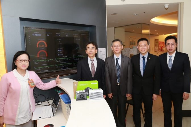
Taipei Veterans General Hospital team
The TVGH team (from L to R): Hsin-Ling Tai, nursing department; Der-Cherng Tarng, chief of the department of medicine; Chen-Tsung Kuo, director of the information department; Yuan-Chia Chu, senior software engineer; and Shuo-Ming Ou, visiting staff in the nephrology division.

“A half-hour window between data analysis still left gaps where a patient may begin experiencing complications that can lead to heart failure,” said Shou-Ming Ou, visiting staff in the nephrology division at TVGH. “So our team worked to find a real-time solution that could receive and compute data generated by dialysis machines within milliseconds.”

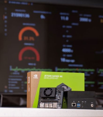
NVIDIA Jetson Xavier NXTo achieve real-time AI inference using streaming data over the course of a four-hour dialysis session, TVGH adopted the Aetina Edge AI Starter Package featuring NVIDIA Jetson Xavier NX, which packs the power to process up to 21 trillion operations per second in a compact module that consumes just 10 watts. The team used NVIDIA TensorRT software to optimize their AI prediction model for inference on the Jetson platform.

By shifting processing to the edge, NVIDIA Jetson also helps TVGH reduce the computation workload on their main servers, freeing up resources to support other AI teams training high-quality medical models.

In addition to the heart failure risk prediction model, the hospital is working on additional AI projects accelerated with the NVIDIA Parabricks genomics software, the NVIDIA FLARE federated learning workflow and the NeMo Megatron framework for natural language processing.

To learn more, hear the TVGH team share their work in a session from the latest NVIDIA GTC.

Subscribe to NVIDIA healthcare news.

The post Detect to Protect: Taiwan Hospital Deploys Real-Time AI Risk Prediction for Kidney Patients appeared first on NVIDIA Blog.

Read More

DALL·E 2 pre-training mitigations

In order to share the magic of DALL·E 2 with a broad audience, we needed to reduce the risks associated with powerful image generation models. To this end, we put various guardrails in place to prevent generated images from violating our content policy.OpenAI Blog

A BetterTransformer for Fast Transformer Inference

tl;dr Transformers achieve state-of-the-art performance for NLP, and are becoming popular for a myriad of other tasks. They are computationally expensive which has been a blocker to their widespread productionisation. Launching with PyTorch 1.12, BetterTransformer implements a backwards-compatible fast path of torch.nn.TransformerEncoder for Transformer Encoder Inference and does not require model authors to modify their models. BetterTransformer improvements can exceed 2x in speedup and throughput for many common execution scenarios. To use BetterTransformer, install PyTorch 1.12 and start using high-quality, high-performance Transformer models with the PyTorch API today.

Diagram of the Transformer Encoder Architecture (from “Attention Is All You Need“). During Inference, the entire module will execute as a single PyTorch-native function.

In this blog post, we share the following topics — Performance Improvements, Backwards compatibility, and Taking advantage of the FastPath. Learn more about these topics below.

Performance Improvements

BetterTransformer launches with accelerated native implementations of MultiHeadAttention and TransformerEncoderLayer for CPUs and GPUs. These fast paths are integrated in the standard PyTorch Transformer APIs, and will accelerate TransformerEncoder, TransformerEncoderLayer and MultiHeadAttention nn.modules. These new modules implement two types of optimizations: (1) fused kernels combine multiple individual operators normally used to implement Transformers to provide a more efficient implementation, and (2) take advantage of sparsity in the inputs to avoid performing unnecessary operations on padding tokens. Padding tokens frequently account for a large fraction of input batches in many Transformer models used for Natural Language Processing.

Backwards compatibility

Advantageously, no model changes are necessary to benefit from the performance boost offered by BetterTransformer. To benefit from fast path execution, inputs and operating conditions must satisfy some access conditions (see below). While the internal implementation of Transformer APIs has changed, PyTorch 1.12 maintains strict compatibility with Transformer modules shipped in previous versions, enabling PyTorch users to use models created and trained with previous PyTorch releases while benefiting from BetterTransformer improvements.

In addition to enabling the PyTorch nn.Modules, BetterTransformer provides improvements for PyTorch libraries. Performance benefits will become available through two different enablement paths:

  1. Transparent acceleration: Current users of PyTorch nn.Modules such as MultiHeadAttention as well as higher-level Transformer components will benefit from the improved performance of the new nn.Modules automatically. An example of this is the visual transformer (ViT) implementation used in the torchvision library (code link).

  2. Torchtext library acceleration: As part of this project, we have optimized Torchtext to build on the PyTorch core API to benefit from BetterTransformer enhancements while maintaining strict and transparent compatibility with previous library versions and models trained with previous Torchtext versions. Using PyTorch Transformers in Torchtext also ensures that Torchtext will benefit from expected future enhancements to the PyTorch Transformer implementation.

Taking advantage of the Fastpath

BetterTransformer is a fastpath for the PyTorch Transformer API. The fastpath is a native, specialized implementation of key Transformer functions for CPU and GPU that applies to common Transformer use cases.

To take advantage of input sparsity (i.e. padding) in accelerating your model (see Figure 2), set the keyword argument enable_nested_tensor=True when instantiating a TransformerEncoder and pass in the src_key_padding_mask argument (which denotes padding tokens) during inference. This requires the padding mask to be contiguous, which is the typical case.

Currently, the BetterTransformer speedup only applies to transformer encoder models used in inference. To benefit from fastpath execution, models must be composed of any of the following components: TransformerEncoder, TransformerEncoderLayer or MultiheadAttention (MHA). Fastpath execution is also subject to some criteria. Most importantly, the model must be executed in inference mode and operate on input tensors that do not collect gradient tape information (e.g., running with torch.no_grad). The full list of conditions can be found at these links for nn.MultiHeadAttention and nn.TransformerEncoder, respectively. If the criteria are not met, control flows to the legacy PyTorch 1.11 Transformer implementation which has the same API, but lacks the fastpath performance boost.

Other transformer models (such as decoder models) which use the PyTorch MultiheadAttention module will benefit from the BetterTransformer fastpath. Planned future work is to expand the end-to-end BetterTransformer fastpath to models based on TransformerDecoder to support popular seq2seq and decoder-only (e.g., OPT) model architectures, and to training.

Speedups

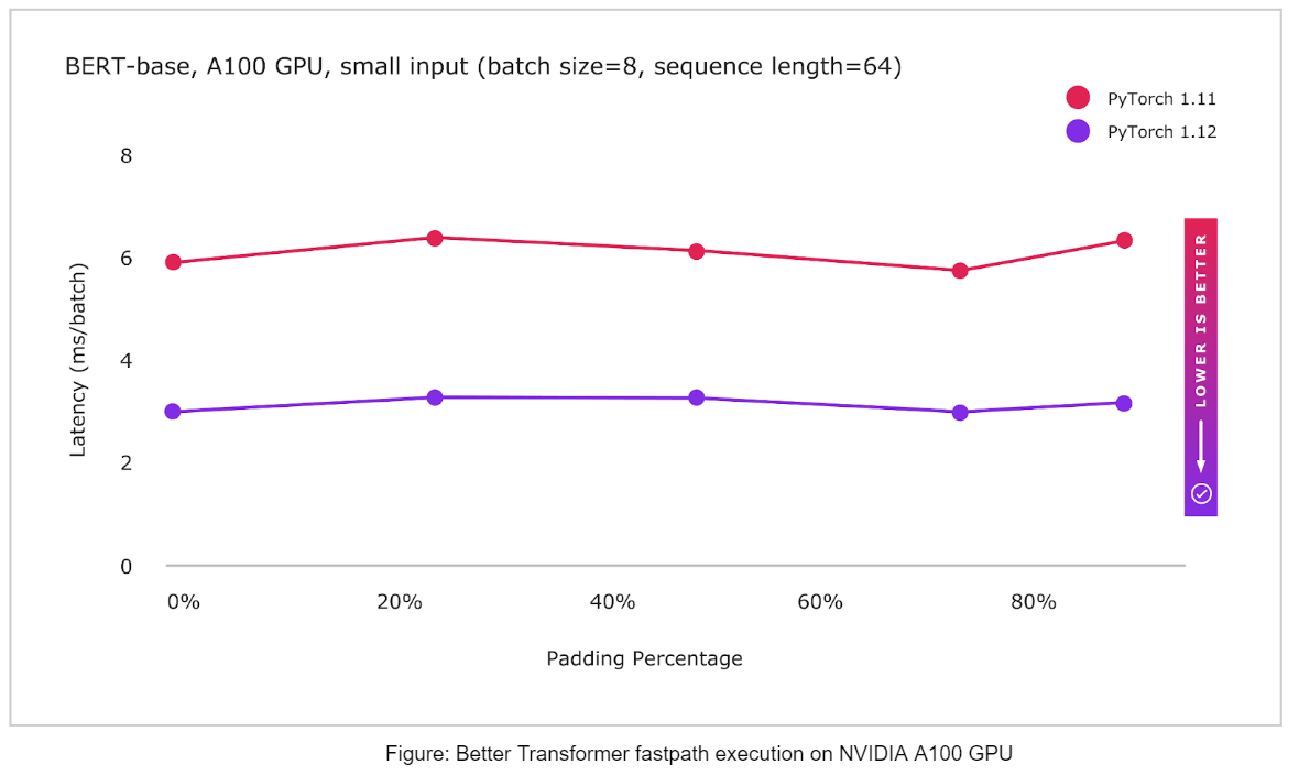
The following graphs show the performance achieved for the BERT-base model with small and large-scale inputs:

Figure 1: PyTorch 1.12 Improvements with BetterTransformer fastpath execution

Figure 2: PyTorch 1.12 Improvements with BetterTransformer fastpath execution
with sparsity optimization enabled by enable_nested_tensor=True

BetterTransformer includes two types of optimization: (1) fused kernels implementing multiple operations more efficiently in a single kernel, and (2) exploiting sparsity by avoiding unnecessary processing on padding tokens. Enhanced performance for small input sizes benefits primarily from the fused kernel implementations, and shows a constant performance improvement regardless of padding amount. While large inputs still benefit from fused kernels, the computation heavy processing limits the benefits that may be obtained by the fused kernels as baseline performance is already closer to the theoretical peak. However, as we increase the amount of padding, performance increases dramatically as increasingly large amounts of computation can be avoided by exploiting the sparsity introduced by padding in NLP workloads.

Future Work

As part of our ongoing work on PyTorch BetterTransformer, we are working on extending BetterTransformer improvements to Transformer Decoders. We aim to expand beyond inference to training as well.

We are partnering to enable BetterTransformer on additional libraries such as FairSeq, MetaSeq, and HuggingFace to benefit all Transformer-based PyTorch models. We’ll provide future updates on the progress of BetterTransformer accelerations for the larger PyTorch ecosystem as part of this blog series.

Acknowledgements: The authors would like to thank Lin Qiao, Ajit Mathews, Andrew Tulloch, Dmytro Dzhulgakov, Natalia Gimelshein, Emad El-Haraty, Mark Saroufim, Adnan Aziz, Geeta Chauhan, and Hamid Shojanazeri for their support, contributions and many helpful suggestions throughout the course of this project, and in the preparation of this blog.

Read More

New library updates in PyTorch 1.12

We are bringing a number of improvements to the current PyTorch libraries, alongside the PyTorch 1.12 release. These updates demonstrate our focus on developing common and extensible APIs across all domains to make it easier for our community to build ecosystem projects on PyTorch.

Summary:

  • TorchVision – Added multi-weight support API, new architectures, model variants, and pretrained weight. See the release notes here.
  • TorchAudio – Introduced beta features including a streaming API, a CTC beam search decoder, and new beamforming modules and methods. See the release notes here.
  • TorchText – Extended support for scriptable BERT tokenizer and added datasets for GLUE benchmark. See the release notes here.
  • TorchRec – Added EmbeddingModule benchmarks, examples for TwoTower Retrieval, inference and sequential embeddings, metrics, improved planner and demonstrated integration with production components. See the release notes here.
  • TorchX – Launch PyTorch trainers developed on local workspaces onto five different types of schedulers. See the release notes here.
  • FBGemm – Added and improved kernels for Recommendation Systems inference workloads, including table batched embedding bag, jagged tensor operations, and other special-case optimizations.

TorchVision v0.13

Multi-weight support API

TorchVision v0.13 offers a new Multi-weight support API for loading different weights to the existing model builder methods:

from torchvision.models import *

# Old weights with accuracy 76.130%
resnet50(weights=ResNet50_Weights.IMAGENET1K_V1)

# New weights with accuracy 80.858%
resnet50(weights=ResNet50_Weights.IMAGENET1K_V2)

# Best available weights (currently alias for IMAGENET1K_V2)
# Note that these weights may change across versions
resnet50(weights=ResNet50_Weights.DEFAULT)

# Strings are also supported
resnet50(weights="IMAGENET1K_V2")

# No weights - random initialization
resnet50(weights=None)

The new API bundles along with the weights important details such as the preprocessing transforms and meta-data such as labels. Here is how to make the most out of it:

from torchvision.io import read_image
from torchvision.models import resnet50, ResNet50_Weights

img = read_image("test/assets/encode_jpeg/grace_hopper_517x606.jpg")

# Step 1: Initialize model with the best available weights
weights = ResNet50_Weights.DEFAULT
model = resnet50(weights=weights)
model.eval()

# Step 2: Initialize the inference transforms
preprocess = weights.transforms()

# Step 3: Apply inference preprocessing transforms
batch = preprocess(img).unsqueeze(0)

# Step 4: Use the model and print the predicted category
prediction = model(batch).squeeze(0).softmax(0)
class_id = prediction.argmax().item()
score = prediction[class_id].item()
category_name = weights.meta["categories"][class_id]
print(f"{category_name}: {100 * score:.1f}%")

You can read more about the new API in the docs. To provide your feedback, please use this dedicated Github issue.

New architectures and model variants

Classification

The Swin Transformer and EfficienetNetV2 are two popular classification models which are often used for downstream vision tasks. This release includes 6 pre-trained weights for their classification variants. Here is how to use the new models:

import torch
from torchvision.models import *

image = torch.rand(1, 3, 224, 224)
model = swin_t(weights="DEFAULT").eval()
prediction = model(image)

image = torch.rand(1, 3, 384, 384)
model = efficientnet_v2_s(weights="DEFAULT").eval()
prediction = model(image)

In addition to the above, we also provide new variants for existing architectures such as ShuffleNetV2, ResNeXt and MNASNet. The accuracies of all the new pre-trained models obtained on ImageNet-1K are seen below:

Model Acc@1 Acc@5
swin_t 81.474 95.776
swin_s 83.196 96.36
swin_b 83.582 96.64
efficientnet_v2_s 84.228 96.878
efficientnet_v2_m 85.112 97.156
efficientnet_v2_l 85.808 97.788
resnext101_64x4d 83.246 96.454
resnext101_64x4d (quantized) 82.898 96.326
shufflenet_v2_x1_5 72.996 91.086
shufflenet_v2_x1_5 (quantized) 72.052 0.700
shufflenet_v2_x2_0 76.230 93.006
shufflenet_v2_x2_0 (quantized) 75.354 92.488
mnasnet0_75 71.180 90.496
mnas1_3 76.506 93.522

We would like to thank Hu Ye for contributing to TorchVision the Swin Transformer implementation.

(BETA) Object Detection and Instance Segmentation

We have introduced 3 new model variants for RetinaNet, FasterRCNN and MaskRCNN that include several post-paper architectural optimizations and improved training recipes. All models can be used similarly:

import torch
from torchvision.models.detection import *

images = [torch.rand(3, 800, 600)]
model = retinanet_resnet50_fpn_v2(weights="DEFAULT")
# model = fasterrcnn_resnet50_fpn_v2(weights="DEFAULT")
# model = maskrcnn_resnet50_fpn_v2(weights="DEFAULT")
model.eval()
prediction = model(images)

Below we present the metrics of the new variants on COCO val2017. In parenthesis we denote the improvement over the old variants:

Model Box mAP Mask mAP
retinanet_resnet50_fpn_v2 41.5 (+5.1)
fasterrcnn_resnet50_fpn_v2 46.7 (+9.7)
maskrcnn_resnet50_fpn_v2 47.4 (+9.5) 41.8 (+7.2)

We would like to thank Ross Girshick, Piotr Dollar, Vaibhav Aggarwal, Francisco Massa and Hu Ye for their past research and contributions to this work.

New pre-trained weights

SWAG weights

The ViT and RegNet model variants offer new pre-trained SWAG (​​Supervised Weakly from hashtAGs) weights. One of the biggest of these models achieves a whopping 88.6% accuracy on ImageNet-1K. We currently offer two versions of the weights: 1) fine-tuned end-to-end weights on ImageNet-1K (highest accuracy) and 2) frozen trunk weights with a linear classifier fit on ImageNet-1K (great for transfer learning). Below we see the detailed accuracies of each model variant:

Model Weights Acc@1 Acc@5
RegNet_Y_16GF_Weights.IMAGENET1K_SWAG_E2E_V1 86.012 98.054
RegNet_Y_16GF_Weights.IMAGENET1K_SWAG_LINEAR_V1 83.976 97.244
RegNet_Y_32GF_Weights.IMAGENET1K_SWAG_E2E_V1 86.838 98.362
RegNet_Y_32GF_Weights.IMAGENET1K_SWAG_LINEAR_V1 84.622 97.48
RegNet_Y_128GF_Weights.IMAGENET1K_SWAG_E2E_V1 88.228 98.682
RegNet_Y_128GF_Weights.IMAGENET1K_SWAG_LINEAR_V1 86.068 97.844
ViT_B_16_Weights.IMAGENET1K_SWAG_E2E_V1 85.304 97.65
ViT_B_16_Weights.IMAGENET1K_SWAG_LINEAR_V1 81.886 96.18
ViT_L_16_Weights.IMAGENET1K_SWAG_E2E_V1 88.064 98.512
ViT_L_16_Weights.IMAGENET1K_SWAG_LINEAR_V1 85.146 97.422
ViT_H_14_Weights.IMAGENET1K_SWAG_E2E_V1 88.552 98.694
ViT_H_14_Weights.IMAGENET1K_SWAG_LINEAR_V1 85.708 97.73

The SWAG weights are released under the Attribution-NonCommercial 4.0 International license. We would like to thank Laura Gustafson, Mannat Singh and Aaron Adcock for their work and support in making the weights available to TorchVision.

Model Refresh

The release of the Multi-weight support API enabled us to refresh the most popular models and offer more accurate weights. We improved on average each model by ~3 points. The new recipe used was learned on top of ResNet50 and its details were covered on a previous blog post.

Model Old weights New weights
efficientnet_b1 78.642 79.838
mobilenet_v2 71.878 72.154
mobilenet_v3_large 74.042 75.274
regnet_y_400mf 74.046 75.804
regnet_y_800mf 76.42 78.828
regnet_y_1_6gf 77.95 80.876
regnet_y_3_2gf 78.948 81.982
regnet_y_8gf 80.032 82.828
regnet_y_16gf 80.424 82.886
regnet_y_32gf 80.878 83.368
regnet_x_400mf 72.834 74.864
regnet_x_800mf 75.212 77.522
regnet_x_1_6gf 77.04 79.668
regnet_x_3_2gf 78.364 81.196
regnet_x_8gf 79.344 81.682
regnet_x_16gf 80.058 82.716
regnet_x_32gf 80.622 83.014
resnet50 76.13 80.858
resnet50 (quantized) 75.92 80.282
resnet101 77.374 81.886
resnet152 78.312 82.284
resnext50_32x4d 77.618 81.198
resnext101_32x8d 79.312 82.834
resnext101_32x8d (quantized) 78.986 82.574
wide_resnet50_2 78.468 81.602
wide_resnet101_2 78.848 82.51

We would like to thank Piotr Dollar, Mannat Singh and Hugo Touvron for their past research and contributions to this work.

New Augmentations, Layers and Losses

This release brings a bunch of new primitives which can be used to produce SOTA models. Some highlights include the addition of AugMix data-augmentation method, the DropBlock layer, the cIoU/dIoU loss and many more. We would like to thank Aditya Oke, Abhijit Deo, Yassine Alouini and Hu Ye for contributing to the project and for helping us maintain TorchVision relevant and fresh.

Documentation

We completely revamped our models documentation to make them easier to browse, and added various key information such as supported image sizes, or image pre-processing steps of pre-trained weights. We now have a main model page with various summary tables of available weights, and each model has a dedicated page. Each model builder is also documented in their own page, with more details about the available weights, including accuracy, minimal image size, link to training recipes, and other valuable info. For comparison, our previous models docs are here. To provide feedback on the new documentation, please use the dedicated Github issue.

TorchAudio v0.12

(BETA) Streaming API

StreamReader is TorchAudio’s new I/O API. It is backed by FFmpeg†, and allows users to:

  • Decode audio and video formats, including MP4 and AAC
  • Handle input forms, such as local files, network protocols, microphones, webcams, screen captures and file-like objects
  • Iterate over and decode chunk-by-chunk, while changing the sample rate or frame rate
  • Apply audio and video filters, such as low-pass filter and image scaling
  • Decode video with Nvidia’s hardware-based decoder (NVDEC)

For usage details, please check out the documentation and tutorials:

† To use StreamReader, FFmpeg libraries are required. Please install FFmpeg. The coverage of codecs depends on how these libraries are configured. TorchAudio official binaries are compiled to work with FFmpeg 4 libraries; FFmpeg 5 can be used if TorchAudio is built from source.

(BETA) CTC Beam Search Decoder

TorchAudio integrates the wav2letter CTC beam search decoder from Flashlight (GitHub). The addition of this inference time decoder enables running end-to-end CTC ASR evaluation using TorchAudio utils.

Customizable lexicon and lexicon-free decoders are supported, and both are compatible with KenLM n-gram language models or without using a language model. TorchAudio additionally supports downloading token, lexicon, and pretrained KenLM files for the LibriSpeech dataset.

For usage details, please check out the documentation and ASR inference tutorial.

(BETA) New Beamforming Modules and Methods

To improve flexibility in usage, the release adds two new beamforming modules under torchaudio.transforms: SoudenMVDR and RTFMVDR. The main differences from MVDR are:

  • Use power spectral density (PSD) and relative transfer function (RTF) matrices as inputs instead of time-frequency masks. The module can be integrated with neural networks that directly predict complex-valued STFT coefficients of speech and noise
  • Add ‘reference_channel’ as an input argument in the forward method, to allow users to select the reference channel in model training or dynamically change the reference channel in inference

Besides the two modules, new function-level beamforming methods are added under torchaudio.functional. These include:

For usage details, please check out the documentation at torchaudio.transforms and torchaudio.functional and the Speech Enhancement with MVDR Beamforming tutorial.

TorchText v0.13

Glue Datasets

We increased the number of datasets in TorchText from 22 to 30 by adding the remaining 8 datasets from the GLUE benchmark (SST-2 was already supported). The complete list of GLUE datasets is as follows:

  • CoLA (paper): Single sentence binary classification acceptability task
  • SST-2 (paper): Single sentence binary classification sentiment task
  • MRPC (paper): Dual sentence binary classification paraphrase task
  • QQP: Dual sentence binary classification paraphrase task
  • STS-B (paper): Single sentence to float regression sentence similarity task
  • MNLI (paper): Sentence ternary classification NLI task
  • QNLI (paper): Sentence binary classification QA and NLI tasks
  • RTE (paper): Dual sentence binary classification NLI task
  • WNLI (paper): Dual sentence binary classification coreference and NLI tasks

Scriptable BERT Tokenizer

TorchText has extended support for scriptable tokenizer by adding the WordPiece tokenizer used in BERT. It is one of the commonly used algorithms for splitting input text into sub-words units and was introduced in Japanese and Korean Voice Search (Schuster et al., 2012).

TorchScriptabilty support would allow users to embed the BERT text-preprocessing natively in C++ without needing the support of python runtime. As TorchText now supports the CMAKE build system to natively link torchtext binaries with application code, users can easily integrate BERT tokenizers for deployment needs.

For usage details, please refer to the corresponding documentation.

TorchRec v0.2.0

EmbeddingModule + DLRM benchmarks

A set of benchmarking tests, showing performance characteristics of TorchRec’s base modules and research models built out of TorchRec.

TwoTower Retrieval Example, with FAISS

We provide an example demonstrating training a distributed TwoTower (i.e. User-Item) Retrieval model that is sharded using TorchRec. The projected item embeddings are added to an IVFPQ FAISS index for candidate generation. The retrieval model and KNN lookup are bundled in a Pytorch model for efficient end-to-end retrieval.

Integrations

We demonstrate that TorchRec works out of the box with many components commonly used alongside PyTorch models in production like systems, such as

  • Training a TorchRec model on Ray Clusters utilizing the Torchx Ray scheduler
  • Preprocessing and DataLoading with NVTabular on DLRM
  • Training a TorchRec model with on-the-fly preprocessing with TorchArrow showcasing RecSys domain UDFs

Sequential Embeddings Example: Bert4Rec

We provide an example, using TorchRec, that reimplements the BERT4REC paper, showcasing EmbeddingCollection for non-pooled embeddings. Using DistributedModelParallel we see a 35% QPS gain over conventional data parallelism.

(Beta) Planner

The TorchRec library includes a built-in planner that selects near optimal sharding plan for a given model. The planner attempts to identify the best sharding plan by evaluating a series of proposals which are statically analyzed and fed into an integer partitioner. The planner is able to automatically adjust plans for a wide range of hardware setups, allowing users to scale performance seamlessly from local development environment to large scale production hardware. See this notebook for a more detailed tutorial.

(Beta) Inference

TorchRec Inference is a C++ library that supports multi-gpu inference. The TorchRec library is used to shard models written and packaged in Python via torch.package (an alternative to TorchScript). The torch.deploy library is used to serve inference from C++ by launching multiple Python interpreters carrying the packaged model, thus subverting the GIL. Two models are provided as examples: DLRM multi-GPU (sharded via TorchRec) and DLRM single-GPU.

(Beta) RecMetrics

RecMetrics is a metrics library that collects common utilities and optimizations for Recommendation models. It extends torchmetrics.

  • A centralized metrics module that allows users to add new metrics
  • Commonly used metrics, including AUC, Calibration, CTR, MSE/RMSE, NE & Throughput
  • Optimization for metrics related operations to reduce the overhead of metric computation
  • Checkpointing

(Prototype) Single process Batched + Fused Embeddings

Previously TorchRec’s abstractions (EmbeddingBagCollection/EmbeddingCollection) over FBGEMM kernels, which provide benefits such as table batching, optimizer fusion, and UVM placement, could only be used in conjunction with DistributedModelParallel. We’ve decoupled these notions from sharding, and introduced the FusedEmbeddingBagCollection, which can be used as a standalone module, with all of the above features, and can also be sharded.

TorchX v0.2.0

TorchX is a job launcher that makes it easier to run PyTorch in distributed training clusters with many scheduler integrations including Kubernetes and Slurm. We’re excited to release TorchX 0.2.0 with a number of improvements. TorchX is currently being used in production in both on-premise and cloud environments.

Check out the quickstart to start launching local and remote jobs.

Workspaces

TorchX now supports workspaces which allows users to easily launch training jobs using their local workspace. TorchX can automatically build a patch with your local training code on top of a base image to minimize iteration time and time to training.

.torchxconfig

Specifying options in .torchxconfig saves you from having to type long CLI commands each time you launch a job. You can also define project level generic configs and drop a config file in your home directory for user-level overrides.

Expanded Scheduler Support

TorchX now supports AWS Batch and Ray (experimental) schedulers in addition to our existing integrations.

Distributed Training On All Schedulers

The TorchX dist.ddp component now works on all schedulers without any configuration. Distributed training workers will automatically discover each other when using torchelastic via the builtin dist.ddp component.

Hyper Parameter Optimization

TorchX integrates with Ax to let you scale hyper-parameter optimizations (HPO) by launching the search trials onto remote clusters.

File and Device Mounts

TorchX now supports remote filesystem mounts and custom devices. This enables your PyTorch jobs to efficiently access cloud storage such as NFS or Lustre. The device mounts enables usage of network accelerators like Infiniband and custom inference/training accelerators.

FBGemm v0.2.0

The FBGEMM library contains optimized kernels meant to improve the performance of PyTorch workloads. We’ve added a number of new features and optimizations over the last few months that we are excited to report.

Inference Table Batched Embedding (TBE)

The table batched embedding bag (TBE) operator is an important base operation for embedding lookup for recommendation system inference on GPU. We added the following enhancements for performance and flexibility:

Alignment restriction removed

  • Embedding dimension * data type size had to be multiple of 4B before and now, it is 1B.

Unified Virtual Memory (UVM) caching kernel optimizations

  • UVM caching kernels now scale linearly with # of tables using UVM caching. Previously, it was having similar overhead as all tables using UVM caching
  • UVM caching kernel overhead is much smaller than before

Inference FP8 Table Batched Embedding (TBE)

The table batched embedding bag (TBE) previously supported FP32, FP16, INT8, INT4, and INT2 embedding weight types. While these weight types work well in many models, we integrate FP8 weight types (in both GPU and CPU operations) to allow for numerical and performance evaluations of FP8 in our models. Compared to INT8, FP8 does not require the additional bias and scale storage and calculations. Additionally, the next generation of H100 GPUs has the FP8 support on Tensor Core (mainly matmul ops).

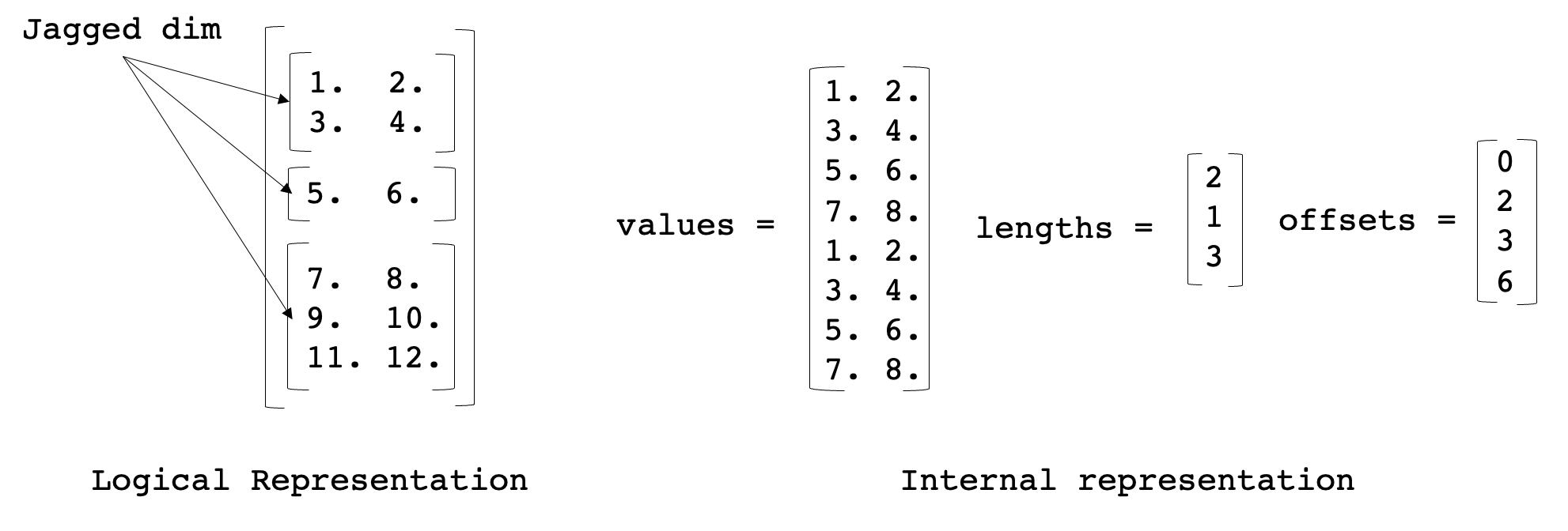
Jagged Tensor Kernels

We added optimized kernels to speed up TorchRec JaggedTensor. The purpose of JaggedTensor is to handle the case where one dimension of the input data is “jagged”, meaning that each consecutive row in a given dimension may be a different length, which is often the case with sparse feature inputs in recommendation systems. The internal representation is shown below:

We added ops for converting jagged tensors from sparse to dense formats and back, performing matrix multiplications with jagged tensors, and elementwise ops.

Optimized permute102-baddbmm-permute102

It is difficult to fuse various matrix multiplications where the batch size is not the batch size of the model, switching the batch dimension is a quick solution. We created the permute102_baddbmm_permute102 operation that switches the first and the second dimension, performs the batched matrix multiplication and then switches back. Currently we only support forward pass with FP16 data type and will support FP32 type and backward pass in the future.

Optimized index_select for dim 0 index selection

index_select is normally used as part of a sparse operation. While PyTorch supports a generic index_select for an arbitrary-dimension index selection, its performance for a special case like the dim 0 index selection is suboptimal. For this reason, we implement a specialized index_select for dim 0. In some cases, we have observed 1.4x performance gain from FBGEMM’s index_select compared to the one from PyTorch (using uniform index distribution).

More about the implementation of influential instances can be found on our GitHub page and tutorials.

Thanks for reading, If you’re interested in these updates and want to join the PyTorch community, we encourage you to join the discussion forums and open GitHub issues. To get the latest news from PyTorch, follow us on Twitter, Medium, YouTube, and LinkedIn.

Cheers!

Team PyTorch

Read More

PyTorch 1.12: TorchArrow, Functional API for Modules and nvFuser, are now available

We are excited to announce the release of PyTorch 1.12 (release note)! This release is composed of over 3124 commits, 433 contributors. Along with 1.12, we are releasing beta versions of AWS S3 Integration, PyTorch Vision Models on Channels Last on CPU, Empowering PyTorch on Intel® Xeon® Scalable processors with Bfloat16 and FSDP API. We want to sincerely thank our dedicated community for your contributions.

Summary:

  • Functional APIs to functionally apply module computation with a given set of parameters
  • Complex32 and Complex Convolutions in PyTorch
  • DataPipes from TorchData fully backward compatible with DataLoader
  • functorch with improved coverage for APIs
  • nvFuser a deep learning compiler for PyTorch
  • Changes to float32 matrix multiplication precision on Ampere and later CUDA hardware
  • TorchArrow, a new beta library for machine learning preprocessing over batch data

Frontend APIs

Introducing TorchArrow

We’ve got a new Beta release ready for you to try and use: TorchArrow. This is a library for machine learning preprocessing over batch data. It features a performant and Pandas-style, easy-to-use API in order to speed up your preprocessing workflows and development.

Currently, it provides a Python DataFrame interface with the following features:

  • High-performance CPU backend, vectorized and extensible User-Defined Functions (UDFs) with Velox
  • Seamless handoff with PyTorch or other model authoring, such as Tensor collation and easily plugging into PyTorch DataLoader and DataPipes
  • Zero copy for external readers via Arrow in-memory columnar format

For more details, please find our 10-min tutorial, installation instructions, API documentation, and a prototype for data preprocessing in TorchRec.

(Beta) Functional API for Modules

PyTorch 1.12 introduces a new beta feature to functionally apply Module computation with a given set of parameters. Sometimes, the traditional PyTorch Module usage pattern that maintains a static set of parameters internally is too restrictive. This is often the case when implementing algorithms for meta-learning, where multiple sets of parameters may need to be maintained across optimizer steps.

The new torch.nn.utils.stateless.functional_call() API allows for:

  • Module computation with full flexibility over the set of parameters used
  • No need to reimplement your module in a functional way
  • Any parameter or buffer present in the module can be swapped with an externally-defined value for use in the call. Naming for referencing parameters / buffers follows the fully-qualified form in the module’s state_dict()

Example:

import torch
from torch import nn
from torch.nn.utils.stateless import functional_call

class MyModule(nn.Module):
    def __init__(self):
        super().__init__()
        self.fc1 = nn.Linear(3, 3)
        self.bn = nn.BatchNorm1d(3)
        self.fc2 = nn.Linear(3, 3)

    def forward(self, x):
        return self.fc2(self.bn(self.fc1(x)))

m = MyModule()

# Define parameter / buffer values to use during module computation.
my_weight = torch.randn(3, 3, requires_grad=True)
my_bias = torch.tensor([1., 2., 3.], requires_grad=True)
params_and_buffers = {
    'fc1.weight': my_weight,
    'fc1.bias': my_bias,
    # Custom buffer values can be used too.
    'bn.running_mean': torch.randn(3),
}

# Apply module computation to the input with the specified parameters / buffers.
inp = torch.randn(5, 3)
output = functional_call(m, params_and_buffers, inp)

(Beta) Complex32 and Complex Convolutions in PyTorch

PyTorch today natively supports complex numbers, complex autograd, complex modules, and numerous complex operations, including linear algebra and Fast Fourier Transform (FFT) operators. Many libraries, including torchaudio and ESPNet, already make use of complex numbers in PyTorch, and PyTorch 1.12 further extends complex functionality with complex convolutions and the experimental complex32 (“complex half”) data type that enables half precision FFT operations. Due to the bugs in CUDA 11.3 package, we recommend using CUDA 11.6 package from wheels if you are using complex numbers.

(Beta) Forward-mode Automatic Differentiation

Forward-mode AD allows the computation of directional derivatives (or equivalently, Jacobian-vector products) eagerly in the forward pass. PyTorch 1.12 significantly improves the operator coverage for forward-mode AD. See our tutorial for more information.

TorchData

BC DataLoader + DataPipe

`DataPipe` from TorchData becomes fully backward compatible with the existing `DataLoader` regarding shuffle determinism and dynamic sharding in both multiprocessing and distributed environments. For more details, please check out the tutorial.

(Beta) AWS S3 Integration

DataPipes based on AWSSDK have been integrated into TorchData. It provides the following features backed by native AWSSDK:

  • Retrieve list of urls from each S3 bucket based on prefix
    • Support timeout to prevent hanging indefinitely
    • Support to specify S3 bucket region
  • Load data from S3 urls
    • Support buffered and multi-part download
    • Support to specify S3 bucket region

AWS native DataPipes are still in the beta phase. And, we will keep tuning them to improve their performance.

(Prototype) DataLoader2

DataLoader2 became available in prototype mode. We are introducing new ways to interact between DataPipes, DataLoading API, and backends (aka ReadingServices). Feature is stable in terms of API, but functionally not complete yet. We welcome early adopters and feedback, as well as potential contributors.

For more details, please checkout the link.

functorch

Inspired by Google JAX, functorch is a library that offers composable vmap (vectorization) and autodiff transforms. It enables advanced autodiff use cases that would otherwise be tricky to express in PyTorch. Examples of these include:

We’re excited to announce functorch 0.2.0 with a number of improvements and new experimental features.

Significantly improved coverage

We significantly improved coverage for functorch.jvp (our forward-mode autodiff API) and other APIs that rely on it (functorch.{jacfwd, hessian}).

(Prototype) functorch.experimental.functionalize

Given a function f, functionalize(f) returns a new function without mutations (with caveats). This is useful for constructing traces of PyTorch functions without in-place operations. For example, you can use make_fx(functionalize(f)) to construct a mutation-free trace of a pytorch function. To learn more, please see the documentation.

For more details, please see our installation instructions, documentation, tutorials, and release notes.

Performance Improvements

Introducing nvFuser, a deep learning compiler for PyTorch

In PyTorch 1.12, Torchscript is updating its default fuser (for Volta and later CUDA accelerators) to nvFuser, which supports a wider range of operations and is faster than NNC, the previous fuser for CUDA devices. A soon to be published blog post will elaborate on nvFuser and show how it speeds up training on a variety of networks.

See the nvFuser documentation for more details on usage and debugging.

Changes to float32 matrix multiplication precision on Ampere and later CUDA hardware

PyTorch supports a variety of “mixed precision” techniques, like the torch.amp (Automated Mixed Precision) module and performing float32 matrix multiplications using the TensorFloat32 datatype on Ampere and later CUDA hardware for faster internal computations. In PyTorch 1.12 we’re changing the default behavior of float32 matrix multiplications to always use full IEEE fp32 precision, which is more precise but slower than using the TensorFloat32 datatype for internal computation. For devices with a particularly high ratio of TensorFloat32 to float32 throughput such as A100, this change in defaults can result in a large slowdown.

If you’ve been using TensorFloat32 matrix multiplications then you can continue to do so by setting torch.backends.cuda.matmul.allow_tf32 = True

which is supported since PyTorch 1.7. Starting in PyTorch 1.12 the new matmul precision API can be used, too: torch.set_float32_matmul_precision(“highest”|”high”|”medium”)

To reiterate, PyTorch’s new default is “highest” precision for all device types. We think this provides better consistency across device types for matrix multiplications. Documentation for the new precision API can be found here. Setting the “high” or “medium” precision types will enable TensorFloat32 on Ampere and later CUDA devices. If you’re updating to PyTorch 1.12 then to preserve the current behavior and faster performance of matrix multiplications on Ampere devices, set precision to “high”.

Using mixed precision techniques is essential for training many modern deep learning networks efficiently, and if you’re already using torch.amp this change is unlikely to affect you. If you’re not familiar with mixed precision training then see our soon to be published “What Every User Should Know About Mixed Precision Training in PyTorch” blogpost.

(Beta) Accelerating PyTorch Vision Models with Channels Last on CPU

Memory formats have a significant impact on performance when running vision models, generally Channels Last is more favorable from a performance perspective due to better data locality. 1.12 includes fundamental concepts of memory formats and demonstrates performance benefits using Channels Last on popular PyTorch vision models on Intel® Xeon® Scalable processors.

  • Enables Channels Last memory format support for the commonly used operators in CV domain on CPU, applicable for both inference and training
  • Provides native level optimization on Channels Last kernels from ATen, applicable for both AVX2 and AVX512
  • Delivers 1.3x to 1.8x inference performance gain over Channels First for TorchVision models on Intel® Xeon® Ice Lake (or newer) CPUs

(Beta) Empowering PyTorch on Intel® Xeon® Scalable processors with Bfloat16

Reduced precision numeric formats like bfloat16 improves PyTorch performance across multiple deep learning training workloads. PyTorch 1.12 includes the latest software enhancements on bfloat16 which applies to a broader scope of user scenarios and showcases even higher performance gains. The main improvements include:

  • 2x hardware compute throughput vs. float32 with the new bfloat16 native instruction VDPBF16PS, introduced on Intel® Xeon® Cooper Lake CPUs
  • 1/2 memory footprint of float32, faster speed for memory bandwidth intensive operators
  • 1.4x to 2.2x inference performance gain over float32 for TorchVision models on Intel® Xeon® Cooper Lake (or newer) CPUs

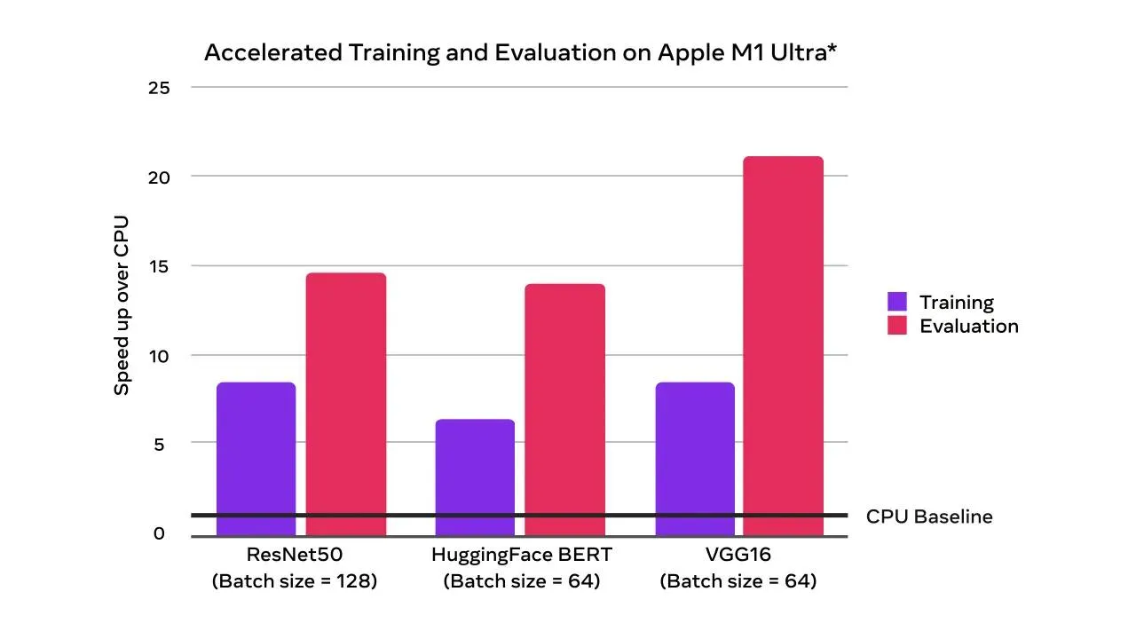
(Prototype) Introducing Accelerated PyTorch Training on Mac

With the PyTorch 1.12 release, developers and researchers can now take advantage of Apple silicon GPUs for significantly faster model training. This unlocks the ability to perform machine learning workflows like prototyping and fine-tuning locally, right on Mac. Accelerated GPU training is enabled using Apple’s Metal Performance Shaders (MPS) as a backend. The benefits include performance speedup from accelerated GPU training and the ability to train larger networks or batch sizes locally. Learn more here.

Accelerated GPU training and evaluation speedups over CPU-only (times faster)

Alongside the new MPS device support, the M1 binaries for Core and Domain libraries that have been available for the last few releases are now an official prototype feature. These binaries can be used to run PyTorch natively on Apple Silicon.

(Prototype) BetterTransformer: Fastpath execution for Transformer Encoder Inference

PyTorch now supports CPU and GPU fastpath implementations (“BetterTransformer”) for several Transformer Encoder modules including TransformerEncoder, TransformerEncoderLayer, and MultiHeadAttention (MHA). The BetterTransformer fastpath architecture Better Transformer is consistently faster – 2x for many common execution scenarios, depending on model and input characteristics. The new BetterTransformer-enabled modules are API compatible with previous releases of the PyTorch Transformer API and will accelerate existing models if they meet fastpath execution requirements, as well as read models trained with previous versions of PyTorch. PyTorch 1.12 includes:

  • BetterTransformer integration for Torchtext’s pretrained RoBERTa and XLM-R models
  • Torchtext which builds on the PyTorch Transformer API
  • Fastpath execution for improved performance by reducing execution overheads with fused kernels which combines multiple operators into a single kernel
  • Option to achieve additional speedups by taking advantage of data sparsity during the processing of padding tokens in natural-language processing (by setting enable_nested_tensor=True when creating a TransformerEncoder)
  • Diagnostics to help users understand why fastpath execution did not occur

Distributed

(Beta) Fully Sharded Data Parallel (FSDP) API

FSDP API helps easily scale large model training by sharding a model’s parameters, gradients and optimizer states across data parallel workers while maintaining the simplicity of data parallelism. The prototype version was released in PyTorch 1.11 with a minimum set of features that helped scaling tests of models with up to 1T parameters.

In this beta release, FSDP API added the following features to support various production workloads. Highlights of the the newly added features in this beta release include:

  1. Universal sharding strategy API – Users can easily change between sharding strategies with a single line change, and thus compare and use DDP (only data sharding), FSDP (full model and data sharding), or Zero2 (only sharding of optimizer and gradients) to optimize memory and performance for their specific training needs
  2. Fine grained mixed precision policies – Users can specify a mix of half and full data types (bfloat16, fp16 or fp32) for model parameters, gradient communication, and buffers via mixed precision policies. Models are automatically saved in fp32 to allow for maximum portability
  3. Transformer auto wrapping policy – allows for optimal wrapping of Transformer based models by registering the models layer class, and thus accelerated training performance
  4. Faster model initialization using device_id init – initialization is performed in a streaming fashion to avoid OOM issues and optimize init performance vs CPU init
  5. Rank0 streaming for full model saving of larger models – Fully sharded models can be saved by all GPU’s streaming their shards to the rank 0 GPU, and the model is built in full state on the rank 0 CPU for saving

For more details and example code, please checkout the documentation and the tutorial.

Thanks for reading, If you’re interested in these updates and want to join the PyTorch community, we encourage you to join the discussion forums and open GitHub issues. To get the latest news from PyTorch, follow us on Twitter, Medium, YouTube, and LinkedIn.

Cheers!

Team PyTorch

Read More

Bringing Machine Learning to every developer’s toolbox

Posted by Laurence Moroney and Josh Gordon for the TensorFlow team

With the release of the recent Stack Overflow Developer Survey, we’re delighted to see the growth of TensorFlow as the most-used ML tool, being adopted by 3 million software developers to enhance their products and solutions using Machine Learning. And we’re only getting started – the survey showed that TensorFlow was the most wanted framework amongst developers, with an estimated 4 million developers wanting to adopt it in the near future.

TensorFlow is now being downloaded over 18M times per month and has amassed 166k stars on GitHub – more than any other ML framework. Within Google, it powers virtually all AI production workflows, including Search, Ads, YouTube, GMail, Maps, Play, Photos, and many more. It also powers production systems at many of the largest companies in the world – Apple, Netflix, Stripe, Tencent, Uber, Roche, LinkedIn, Twitter, Baidu, Orange, LVMH, and countless others. And every month, over 3,000 new scientific publications that mention TensorFlow or Keras are being indexed by Google Scholar, including important applied science like the CANDLE research into understanding cancer.

We continue to grow the family of products and open source services that make up the Google AI/ML ecosystem. In recent years, we learned that a single universal framework could not work for all scenarios – in particular, the needs of production and cutting edge research are often in conflict. So we created JAX, a minimalistic API for distributed numerical computing to power the next era of scientific computing research. JAX is excellent for pushing new frontiers: reaching new scales of parallelism, advancing new algorithms and architectures, and developing new compilers and systems. The adoption of JAX by researchers has been exciting, and advances such as AlphaFold and Imagen underscore this.

In this new multi-framework world, TensorFlow is our answer to the needs of applied ML developers – engineers who need to build and deploy reliable, stable, performant ML systems, at any scale, and for any platform. Our vision is to create a cohesive ecosystem where researchers and engineers can leverage components that work together regardless of the framework where they originated. We’ve already made strides towards JAX and TensorFlow interoperability, in particular via jax2tf. Researchers who develop JAX models will be able to bring them to production via the tools of the TensorFlow platform.

Going forward, we intend to continue to develop TensorFlow as the best-in-class platform for applied ML, side-by-side with JAX to push the boundaries of ML research. We will continue to invest in both ML frameworks to drive forward research and applications for our millions of users.

There’s lots of great stuff baking that we can’t wait to share with you, so watch this blog for more details!

PS: Interested in working on any of our AI and ML frameworks? We’re hiring.

Read More

Inspect your data labels with a visual, no code tool to create high-quality training datasets with Amazon SageMaker Ground Truth Plus

Launched at AWS re:Invent 2021, Amazon SageMaker Ground Truth Plus helps you create high-quality training datasets by removing the undifferentiated heavy lifting associated with building data labeling applications and managing the labeling workforce. All you do is share data along with labeling requirements, and Ground Truth Plus sets up and manages your data labeling workflow based on these requirements. From there, an expert workforce that is trained on a variety of machine learning (ML) tasks performs data labeling. You don’t even need deep ML expertise or knowledge of workflow design and quality management to use Ground Truth Plus.

Building a high-quality training dataset for your ML algorithm is an iterative process. ML practitioners often build custom systems to inspect data labels because accurately labeled data is critical to ML model quality. To ensure you get high-quality training data, Ground Truth Plus provides you with a built-in user interface (Review UI) to inspect the quality of data labels and provide feedback on data labels until you’re satisfied that the labels accurately represent the ground truth, or what is directly observable in the real world.

This post walks you through steps to create a project team and use several new built-in features of the Review UI tool to efficiently complete your inspection of a labeled dataset. The walkthrough assumes that you have an active Ground Truth Plus labeling project. For more information, see Amazon SageMaker Ground Truth Plus – Create Training Datasets Without Code or In-house Resources.

Set up a project team

A project team provides access to the members from your organization to inspect data labels using the Review UI tool. To set up a project team, complete the following steps:

  1. On the Ground Truth Plus console, choose Create project team.
  2. Select Create a new Amazon Cognito user group . If you already have an existing Amazon Cognito user group, select the Import members option.
  3. For Amazon Cognito user group name, enter a name. This name can’t be changed.
  4. For Email addresses, enter the email addresses of up to 50 team members, separated by commas.
  5. Choose Create project team.

Your team members will receive an email inviting them to join the Ground Truth Plus project team. From there, they can log in to the Ground Truth Plus project portal to review the data labels.

Inspect labeled dataset quality

Now let’s dive into a video object tracking example using CBCL StreetScenes dataset.

After the data in your batch has been labeled, the batch is marked as Ready for review.

Select the batch and choose Review batch. You’re redirected to the Review UI. You have the flexibility to choose a different sampling rate for each batch you review. For instance, in our example batch, we have a total of five videos. You can specify if you want to review only a subset of these five videos or all of them.

Now let’s look at the different functionalities within the Review UI that will help you in inspecting the quality of the labeled dataset at a faster pace, and providing feedback on the quality:

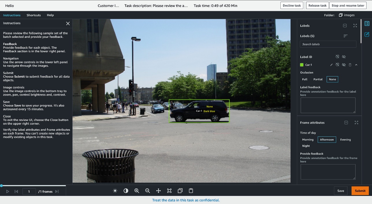
  • Filter the labels based on label category – Within the Review UI, in the right-hand pane, you can filter the labels based on their label category. This feature comes in handy when there are multiple label categories (for example, Vehicles, Pedestrians, and Poles) in a dense dataset object, and you want to view labels for one label category at a time. For example, let’s focus on the Car label category. Enter the Car label category in the right pane to filter for all annotations of only type Car. The following screenshots show the Review UI view before and after applying the filter.
  • Overlay associated annotated attribute values – Each label can be assigned attributes to be annotated. For example, for the label category Car , say you want to ask the workers to also annotate the Color  and Occlusion attributes for each label instance. When you load the Review UI, you will see the corresponding attributes under each label instance on the right pane. But what if you want to see these attribute annotations directly on the image instead? You select the label Car:1 , and to overlay the attribute annotations for Car:1 , you press Ctrl+A.
    Now you will see the annotation Dark Blue for the Color attribute and annotation None for the Occlusion attribute directly displayed on the image next to the Car:1 bounding box. Now you can easily verify that Car:1 was marked as Dark Blue, with no occlusion just from looking at the image instead of having to locate Car:1 on the right pane to see the attribute annotations.
  • Leave feedback at the label level – For each label, you can leave feedback at the label level in that label’s Label feedback free string attribute. For example, in this image, Car:1 looks more black than dark blue. You can relay this discrepancy as feedback for Car:1 using the Label feedback field to track the comment to that label on that frame. Our internal quality control team will review this feedback and introduce changes to the annotation process and label policies, and train the annotators as required.
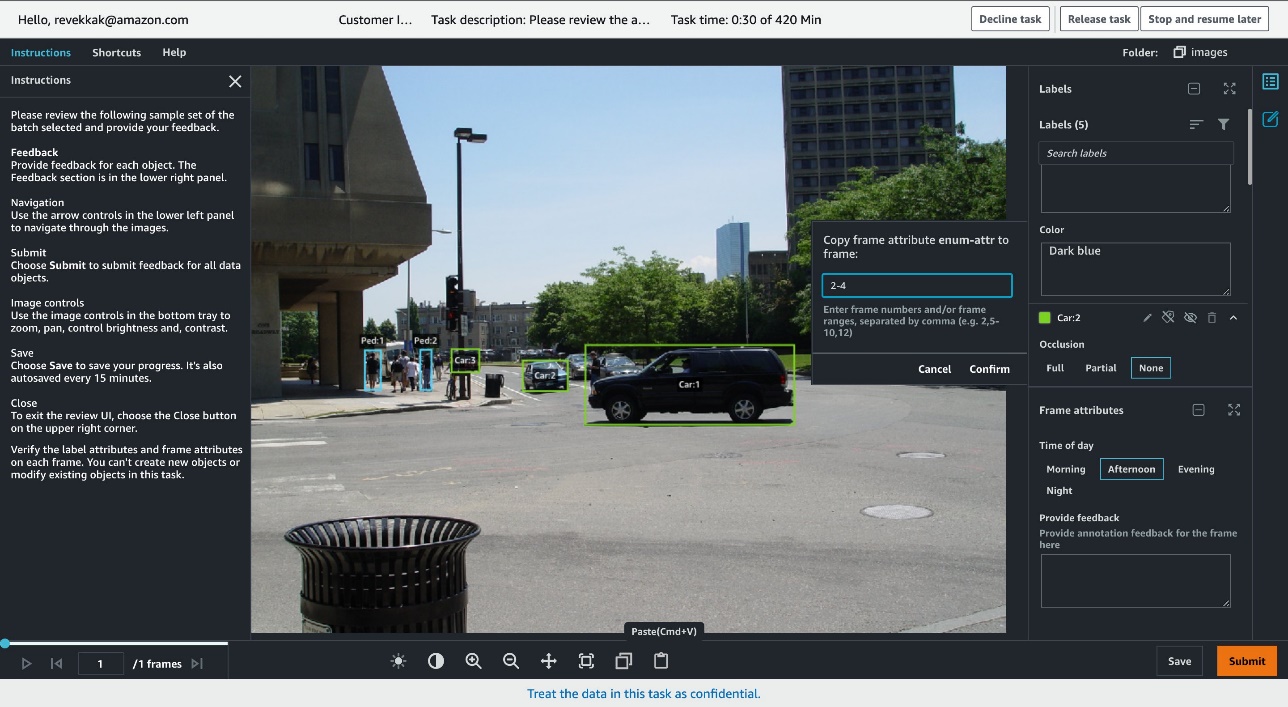
  • Leave feedback at the frame level – Similarly, for each frame, you can leave feedback at the frame level under that frame’s Frame feedback free string attribute. In this case, the annotations for Car and Pedestrian classes look correct and well implemented in this frame. You can relay this positive feedback using the Provide feedback field, and your comment is linked to this frame.
  • Copy the annotation feedback to other frames – You can copy both label-level and frame-level feedback to other frames if you right-click that attribute. This feature is useful when you want to duplicate the same feedback across frames for that label, or apply the same frame-level feedback to several frames. This feature allows you to quickly complete the inspection of data labels.
  • Approve or reject each dataset object – For each dataset object you review, you have the option to either choose Approve if you’re satisfied with the annotations or choose Reject if you’re not satisfied and want those annotations reworked. When you choose Submit, you’re presented with the option to approve or reject the video you just reviewed. In either case, you can provide additional commentary:

    • If you choose Approve, the commentary is optional.
    • If you choose Reject, commentary is required and we suggest providing detailed feedback. Your feedback will be reviewed by a dedicated Ground Truth Plus quality control team, who will take corrective actions to avoid similar mistakes in subsequent videos.

After you submit the video with your feedback, you’re redirected back to the project detail page in the project portal, where you can view the number of rejected objects under the Rejected objects column and the error rate, which is calculated as the number of accepted objects out of reviewed objects under the Acceptance rate column for each batch in your project. For example, for batch 1 in the following screenshot, the acceptance rate is 80% because four objects were accepted out of the five reviewed objects.

Conclusion

A high-quality training dataset is critical for achieving your ML initiatives. With Ground Truth Plus, you now have an enhanced built-in Review UI tool that removes the undifferentiated heavy lifting associated with building custom tools to review the quality of the labeled dataset. This post walked you through how to set up a project team and use the new built-in features of the Review UI tool. Visit the Ground Truth Plus console to get started.

As always, AWS welcomes feedback. Please submit any comments or questions.


About the Author

Manish Goel is the Product Manager for Amazon SageMaker Ground Truth Plus. He is focused on building products that make it easier for customers to adopt machine learning. In his spare time, he enjoys road trips and reading books.

Revekka Kostoeva is a Software Developer Engineer at Amazon AWS where she works on customer facing and internal solutions to expand the breadth and scalability of Sagemaker Ground Truth services. As a researcher, she is driven to improve the tools of the trade to drive innovation forward.

Read More