Today, in partnership with EMBL’s European Bioinformatics Institute (EMBL-EBI), we’re now releasing predicted structures for nearly all catalogued proteins known to science, which will expand the AlphaFold DB by over 200x – from nearly 1 million structures to over 200 million structures – with the potential to dramatically increase our understanding of biology.Read More
Look and Talk: Natural Conversations with Google Assistant
In natural conversations, we don’t say people’s names every time we speak to each other. Instead, we rely on contextual signaling mechanisms to initiate conversations, and eye contact is often all it takes. Google Assistant, now available in more than 95 countries and over 29 languages, has primarily relied on a hotword mechanism (“Hey Google” or “OK Google”) to help more than 700 million people every month get things done across Assistant devices. As virtual assistants become an integral part of our everyday lives, we’re developing ways to initiate conversations more naturally.
At Google I/O 2022, we announced Look and Talk, a major development in our journey to create natural and intuitive ways to interact with Google Assistant-powered home devices. This is the first multimodal, on-device Assistant feature that simultaneously analyzes audio, video, and text to determine when you are speaking to your Nest Hub Max. Using eight machine learning models together, the algorithm can differentiate intentional interactions from passing glances in order to accurately identify a user’s intent to engage with Assistant. Once within 5ft of the device, the user may simply look at the screen and talk to start interacting with the Assistant.
We developed Look and Talk in alignment with our AI Principles. It meets our strict audio and video processing requirements, and like our other camera sensing features, video never leaves the device. You can always stop, review and delete your Assistant activity at myactivity.google.com. These added layers of protection enable Look and Talk to work just for those who turn it on, while keeping your data safe.
 |
| Google Assistant relies on a number of signals to accurately determine when the user is speaking to it. On the right is a list of signals used with indicators showing when each signal is triggered based on the user’s proximity to the device and gaze direction. |
Modeling Challenges
The journey of this feature began as a technical prototype built on top of models developed for academic research. Deployment at scale, however, required solving real-world challenges unique to this feature. It had to:
- Support a range of demographic characteristics (e.g., age, skin tones).
- Adapt to the ambient diversity of the real world, including challenging lighting (e.g., backlighting, shadow patterns) and acoustic conditions (e.g., reverberation, background noise).
- Deal with unusual camera perspectives, since smart displays are commonly used as countertop devices and look up at the user(s), unlike the frontal faces typically used in research datasets to train models.
- Run in real-time to ensure timely responses while processing video on-device.
The evolution of the algorithm involved experiments with approaches ranging from domain adaptation and personalization to domain-specific dataset development, field-testing and feedback, and repeated tuning of the overall algorithm.
Technology Overview
A Look and Talk interaction has three phases. In the first phase, Assistant uses visual signals to detect when a user is demonstrating an intent to engage with it and then “wakes up” to listen to their utterance. The second phase is designed to further validate and understand the user’s intent using visual and acoustic signals. If any signal in the first or second processing phases indicates that it isn’t an Assistant query, Assistant returns to standby mode. These two phases are the core Look and Talk functionality, and are discussed below. The third phase of query fulfillment is typical query flow, and is beyond the scope of this blog.
Phase One: Engaging with Assistant
The first phase of Look and Talk is designed to assess whether an enrolled user is intentionally engaging with Assistant. Look and Talk uses face detection to identify the user’s presence, filters for proximity using the detected face box size to infer distance, and then uses the existing Face Match system to determine whether they are enrolled Look and Talk users.
For an enrolled user within range, an custom eye gaze model determines whether they are looking at the device. This model estimates both the gaze angle and a binary gaze-on-camera confidence from image frames using a multi-tower convolutional neural network architecture, with one tower processing the whole face and another processing patches around the eyes. Since the device screen covers a region underneath the camera that would be natural for a user to look at, we map the gaze angle and binary gaze-on-camera prediction to the device screen area. To ensure that the final prediction is resilient to spurious individual predictions and involuntary eye blinks and saccades, we apply a smoothing function to the individual frame-based predictions to remove spurious individual predictions.
 |
| Eye-gaze prediction and post-processing overview. |
We enforce stricter attention requirements before informing users that the system is ready for interaction to minimize false triggers, e.g., when a passing user briefly glances at the device. Once the user looking at the device starts speaking, we relax the attention requirement, allowing the user to naturally shift their gaze.
The final signal necessary in this processing phase checks that the Face Matched user is the active speaker. This is provided by a multimodal active speaker detection model that takes as input both video of the user’s face and the audio containing speech, and predicts whether they are speaking. A number of augmentation techniques (including RandAugment, SpecAugment, and augmenting with AudioSet sounds) helps improve prediction quality for the in-home domain, boosting end-feature performance by over 10%.The final deployed model is a quantized, hardware-accelerated TFLite model, which uses five frames of context for the visual input and 0.5 seconds for the audio input.
 |
| Active speaker detection model overview: The two-tower audiovisual model provides the “speaking” probability prediction for the face. The visual network auxiliary prediction pushes the visual network to be as good as possible on its own, improving the final multimodal prediction. |
Phase Two: Assistant Starts Listening
In phase two, the system starts listening to the content of the user’s query, still entirely on-device, to further assess whether the interaction is intended for Assistant using additional signals. First, Look and Talk uses Voice Match to further ensure that the speaker is enrolled and matches the earlier Face Match signal. Then, it runs a state-of-the-art automatic speech recognition model on-device to transcribe the utterance.
The next critical processing step is the intent understanding algorithm, which predicts whether the user’s utterance was intended to be an Assistant query. This has two parts: 1) a model that analyzes the non-lexical information in the audio (i.e., pitch, speed, hesitation sounds) to determine whether the utterance sounds like an Assistant query, and 2) a text analysis model that determines whether the transcript is an Assistant request. Together, these filter out queries not intended for Assistant. It also uses contextual visual signals to determine the likelihood that the interaction was intended for Assistant.
 |
| Overview of the semantic filtering approach to determine if a user utterance is a query intended for the Assistant. |
Finally, when the intent understanding model determines that the user utterance was likely meant for Assistant, Look and Talk moves into the fulfillment phase where it communicates with the Assistant server to obtain a response to the user’s intent and query text.
Performance, Personalization and UX
Each model that supports Look and Talk was evaluated and improved in isolation and then tested in the end-to-end Look and Talk system. The huge variety of ambient conditions in which Look and Talk operates necessitates the introduction of personalization parameters for algorithm robustness. By using signals obtained during the user’s hotword-based interactions, the system personalizes parameters to individual users to deliver improvements over the generalized global model. This personalization also runs entirely on-device.
Without a predefined hotword as a proxy for user intent, latency was a significant concern for Look and Talk. Often, a strong enough interaction signal does not occur until well after the user has started speaking, which can add hundreds of milliseconds of latency, and existing models for intent understanding add to this since they require complete, not partial, queries. To bridge this gap, Look and Talk completely forgoes streaming audio to the server, with transcription and intent understanding being on-device. The intent understanding models can work off of partial utterances. This results in an end-to-end latency comparable with current hotword-based systems.
The UI experience is based on user research to provide well-balanced visual feedback with high learnability. This is illustrated in the figure below.
 |
| Left: The spatial interaction diagram of a user engaging with Look and Talk. Right: The User Interface (UI) experience. |
We developed a diverse video dataset with over 3,000 participants to test the feature across demographic subgroups. Modeling improvements driven by diversity in our training data improved performance for all subgroups.
Conclusion
Look and Talk represents a significant step toward making user engagement with Google Assistant as natural as possible. While this is a key milestone in our journey, we hope this will be the first of many improvements to our interaction paradigms that will continue to reimagine the Google Assistant experience responsibly. Our goal is to make getting help feel natural and easy, ultimately saving time so users can focus on what matters most.
Acknowledgements
This work involved collaborative efforts from a multidisciplinary team of software engineers, researchers, UX, and cross-functional contributors. Key contributors from Google Assistant include Alexey Galata, Alice Chuang, Barbara Wang, Britanie Hall, Gabriel Leblanc, Gloria McGee, Hideaki Matsui, James Zanoni, Joanna (Qiong) Huang, Krunal Shah, Kavitha Kandappan, Pedro Silva, Tanya Sinha, Tuan Nguyen, Vishal Desai, Will Truong, Yixing Cai, Yunfan Ye; from Research including Hao Wu, Joseph Roth, Sagar Savla, Sourish Chaudhuri, Susanna Ricco. Thanks to Yuan Yuan and Caroline Pantofaru for their leadership, and everyone on the Nest, Assistant, and Research teams who provided invaluable input toward the development of Look and Talk.
How silicon innovation became the ‘secret sauce’ behind AWS’s success
Nafea Bshara, AWS vice president and distinguished engineer, discusses Annapurna Lab’s path to silicon success; Annapurna co-founder will be a featured speaker in August 3 AWS Silicon Innovation Day virtual event.Read More
Integrate Amazon SageMaker Data Wrangler with MLOps workflows
As enterprises move from running ad hoc machine learning (ML) models to using AI/ML to transform their business at scale, the adoption of ML Operations (MLOps) becomes inevitable. As shown in the following figure, the ML lifecycle begins with framing a business problem as an ML use case followed by a series of phases, including data preparation, feature engineering, model building, deployment, continuous monitoring, and retraining. For many enterprises, a lot of these steps are still manual and loosely integrated with each other. Therefore, it’s important to automate the end-to-end ML lifecycle, which enables frequent experiments to drive better business outcomes. Data preparation is one of the crucial steps in this lifecycle, because the ML model’s accuracy depends on the quality of the training dataset.

Data scientists and ML engineers spend somewhere between 70–80% of their time collecting, analyzing, cleaning, and transforming data required for model training. Amazon SageMaker Data Wrangler is a fully managed capability of Amazon SageMaker that makes it faster for data scientists and ML engineers to analyze and prepare data for their ML projects with little to no code. When it comes to operationalizing an end-to-end ML lifecycle, data preparation is almost always the first step in the process. Given that there are many ways to build an end-to-end ML pipeline, in this post we discuss how you can easily integrate Data Wrangler with some of the well-known workflow automation and orchestration technologies.
Solution overview
In this post, we demonstrate how users can integrate data preparation using Data Wrangler with Amazon SageMaker Pipelines, AWS Step Functions, and Apache Airflow with Amazon Managed Workflow for Apache Airflow (Amazon MWAA). Pipelines is a SageMaker feature that is a purpose-built and easy-to-use continuous integration and continuous delivery (CI/CD) service for ML. Step Functions is a serverless, low-code visual workflow service used to orchestrate AWS services and automate business processes. Amazon MWAA is a managed orchestration service for Apache Airflow that makes it easier to operate end-to-end data and ML pipelines.
For demonstration purposes, we consider a use case to prepare data to train an ML model with the SageMaker built-in XGBoost algorithm that will help us identify fraudulent vehicle insurance claims. We used a synthetically generated set of sample data to train the model and create a SageMaker model using the model artifacts from the training process. Our goal is to operationalize this process end to end by setting up an ML workflow. Although ML workflows can be more elaborate, we use a minimal workflow for demonstration purposes. The first step of the workflow is data preparation with Data Wrangler, followed by a model training step, and finally a model creation step. The following diagram illustrates our solution workflow.

In the following sections, we walk you through how to set up a Data Wrangler flow and integrate Data Wrangler with Pipelines, Step Functions, and Apache Airflow.
Set up a Data Wrangler flow
We start by creating a Data Wrangler flow, also called a data flow, using the data flow UI via the Amazon SageMaker Studio IDE. Our sample dataset consists of two data files: claims.csv and customers.csv, which are stored in an Amazon Simple Storage Service (Amazon S3) bucket. We use the data flow UI to apply Data Wrangler’s built-in transformations such categorical encoding, string formatting, and imputation to the feature columns in each of these files. We also apply custom transformation to a few feature columns using a few lines of custom Python code with Pandas DataFrame. The following screenshot shows the transforms applied to the claims.csv file in the data flow UI.

Finally, we join the results of the applied transforms of the two data files to generate a single training dataset for our model training. We use Data Wrangler’s built-in join datasets capability, which lets us perform SQL-like join operations on tabular data. The following screenshot shows the data flow in the data flow UI in Studio. For step-by-step instructions to create the data flow using Data Wrangler, refer to the GitHub repository.

You can now use the data flow (.flow) file to perform data transformations on our raw data files. The data flow UI can automatically generate Python notebooks for us to use and integrate directly with Pipelines using the SageMaker SDK. For Step Functions, we use the AWS Step Functions Data Science Python SDK to integrate our Data Wrangler processing with a Step Functions pipeline. For Amazon MWAA, we use a custom Airflow operator and the Airflow SageMaker operator. We discuss each of these approaches in detail in the following sections.
Integrate Data Wrangler with Pipelines
SageMaker Pipelines is a native workflow orchestration tool for building ML pipelines that take advantage of direct SageMaker integration. Along with the SageMaker model registry, Pipelines improves the operational resilience and reproducibility of your ML workflows. These workflow automation components enable you to easily scale your ability to build, train, test, and deploy hundreds of models in production; iterate faster; reduce errors due to manual orchestration; and build repeatable mechanisms. Each step in the pipeline can keep track of the lineage, and intermediate steps can be cached for quickly rerunning the pipeline. You can create pipelines using the SageMaker Python SDK.
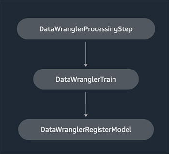
A workflow built with SageMaker pipelines consists of a sequence of steps forming a Directed Acyclic Graph (DAG). In this example, we begin with a processing step, which runs a SageMaker Processing job based on the Data Wrangler’s flow file to create a training dataset. We then continue with a training step, where we train an XGBoost model using SageMaker’s built-in XGBoost algorithm and the training dataset created in the previous step. After a model has been trained, we end this workflow with a RegisterModel step to register the trained model with the SageMaker model registry.
Installation and walkthrough
To run this sample, we use a Jupyter notebook running Python3 on a Data Science kernel image in a Studio environment. You can also run it on a Jupyter notebook instance locally on your machine by setting up the credentials to assume the SageMaker execution role. The notebook is lightweight and can be run on an ml.t3.medium instance. Detailed step-by-step instructions can be found in the GitHub repository.
You can either use the export feature in Data Wrangler to generate the Pipelines code, or build your own script from scratch. In our sample repository, we use a combination of both approaches for simplicity. At a high level, the following are the steps to build and run the Pipelines workflow:
- Generate a flow file from Data Wrangler or use the setup script to generate a flow file from a preconfigured template.
- Create an Amazon Simple Storage Service (Amazon S3) bucket and upload your flow file and input files to the bucket. In our sample notebook, we use the SageMaker default S3 bucket.
- Follow the instructions in the notebook to create a Processor object based on the Data Wrangler flow file, and an Estimator object with the parameters of the training job.
- In our example, because we only use SageMaker features and the default S3 bucket, we can use Studio’s default execution role. The same AWS Identity and Access Management (IAM) role is assumed by the pipeline run, the processing job, and the training job. You can further customize the execution role according to minimum privilege.
- Continue with the instructions to create a pipeline with steps referencing the Processor and Estimator objects, and then run the pipeline. The processing and training jobs run on SageMaker managed environments and take a few minutes to complete.
- In Studio, you can see the pipeline details monitor the pipeline run. You can also monitor the underlying processing and training jobs from the SageMaker console or from Amazon CloudWatch.
Integrate Data Wrangler with Step Functions
With Step Functions, you can express complex business logic as low-code, event-driven workflows that connect different AWS services. The Step Functions Data Science SDK is an open-source library that allows data scientists to create workflows that can preprocess datasets and build, deploy, and monitor ML models using SageMaker and Step Functions. Step Functions is based on state machines and tasks. Step Functions creates workflows out of steps called states, and expresses that workflow in the Amazon States Language. When you create a workflow using the Step Functions Data Science SDK, it creates a state machine representing your workflow and steps in Step Functions.
For this use case, we built a Step Functions workflow based on the common pattern used in this post that includes a processing step, training step, and RegisterModel step. In this case, we import these steps from the Step Functions Data Science Python SDK. We chain these steps in the same order to create a Step Functions workflow. The workflow uses the flow file that was generated from Data Wrangler, but you can also use your own Data Wrangler flow file. We reuse some code from the Data Wrangler export feature for simplicity. We run the data preprocessing logic generated by Data Wrangler flow file to create a training dataset, train a model using the XGBoost algorithm, and save the trained model artifact as a SageMaker model. Additionally, in the GitHub repo, we also show how Step Functions allows us to try and catch errors, and handle failures and retries with FailStateStep and CatchStateStep.
The resulting flow diagram, as shown in the following screenshot, is available on the Step Functions console after the workflow has started. This helps data scientists and engineers visualize the entire workflow and every step within it, and access the linked CloudWatch logs for every step.

Installation and walkthrough
To run this sample, we use a Python notebook running with a Data Science kernel in a Studio environment. You can also run it on a Python notebook instance locally on your machine by setting up the credentials to assume the SageMaker execution role. The notebook is lightweight and can be run on a t3 medium instance for example. Detailed step-by-step instructions can be found in the GitHub repository.
You can either use the export feature in Data Wrangler to generate the Pipelines code and modify it for Step Functions or build your own script from scratch. In our sample repository, we use a combination of both approaches for simplicity. At a high level, the following are the steps to build and run the Step Functions workflow:
- Generate a flow file from Data Wrangler or use the setup script to generate a flow file from a preconfigured template.
- Create an S3 bucket and upload your flow file and input files to the bucket.
- Configure your SageMaker execution role with the required permissions as mentioned earlier. Refer to the GitHub repository for detailed instructions.
- Follow the instructions to run the notebook in the repository to start a workflow. The processing job runs on a SageMaker-managed Spark environment and can take few minutes to complete.
- Go to Step Functions console and track the workflow visually. You can also navigate to the linked CloudWatch logs to debug errors.
Let’s review some important sections of the code here. To define the workflow, we first define the steps in the workflow for the Step Function state machine. The first step is the data_wrangler_step for data processing, which uses the Data Wrangler flow file as an input to transform the raw data files. We also define a model training step and a model creation step named training_step and model_step, respectively. Finally, we create a workflow by chaining all the steps we created, as shown in the following code:
In our example, we built the workflow to take job names as parameters because they’re unique and need to be randomly generated during every pipeline run. We pass these names when the workflow runs. You can also schedule Step Functions workflow to run using CloudWatch (see Schedule a Serverless Workflow with AWS Step Functions and Amazon CloudWatch), invoked using Amazon S3 Events, or invoked from Amazon EventBridge (see Create an EventBridge rule that triggers a Step Functions workflow). For demonstration purposes, we can invoke the Step Functions workflow from the Step Functions console UI or using the following code from the notebook.
Integrate Data Wrangler with Apache Airflow
Another popular way of creating ML workflows is using Apache Airflow. Apache Airflow is an open-source platform that allows you to programmatically author, schedule, and monitor workflows. Amazon MWAA makes it easy to set up and operate end-to-end ML pipelines with Apache Airflow in the cloud at scale. An Airflow pipeline consists of a sequence of tasks, also referred to as a workflow. A workflow is defined as a DAG that encapsulates the tasks and the dependencies between them, defining how they should run within the workflow.
We created an Airflow DAG within an Amazon MWAA environment to implement our MLOps workflow. Each task in the workflow is an executable unit, written in Python programming language, that performs some action. A task can either be an operator or a sensor. In our case, we use an Airflow Python operator along with SageMaker Python SDK to run the Data Wrangler Python script, and use Airflow’s natively supported SageMaker operators to train the SageMaker built-in XGBoost algorithm and create the model from the resulting artifacts. We also created a helpful custom Data Wrangler operator (SageMakerDataWranglerOperator) for Apache Airflow, which you can use to process Data Wrangler flow files for data processing without the need for any additional code.
The following screenshot shows the Airflow DAG with five steps to implement our MLOps workflow.

The Start step uses a Python operator to initialize configurations for the rest of the steps in the workflow. SageMaker_DataWrangler_Step uses SageMakerDataWranglerOperator and the data flow file we created earlier. SageMaker_training_step and SageMaker_create_model_step use the built-in SageMaker operators for model training and model creation, respectively. Our Amazon MWAA environment uses the smallest instance type (mw1.small), because the bulk of the processing is done via Processing jobs, which uses its own instance type that can be defined as configuration parameters within the workflow.
Installation and walkthrough
Detailed step-by-step installation instructions to deploy this solution can be found in our GitHub repository. We used a Jupyter notebook with Python code cells to set up the Airflow DAG. Assuming you have already generated the data flow file, the following is a high-level overview of the installation steps:
- Create an S3 bucket and subsequent folders required by Amazon MWAA.
- Create an Amazon MWAA environment. Note that we used Airflow version 2.0.2 for this solution.
- Create and upload a
requirements.txtfile with all the Python dependencies required by the Airflow tasks and upload it to the/requirementsdirectory within the Amazon MWAA primary S3 bucket. This is used by the managed Airflow environment to install the Python dependencies. - Upload the
SMDataWranglerOperator.pyfile to the/dagsdirectory. This Python script contains code for the custom Airflow operator for Data Wrangler. This operator can be used for tasks to process any .flow file. - Create and upload the
config.pyscript to the/dagsdirectory. This Python script is used for the first step of our DAG to create configuration objects required by the remaining steps of the workflow. - Finally, create and upload the
ml_pipelines.pyfile to the/dagsdirectory. This script contains the DAG definition for the Airflow workflow. This is where we define each of the tasks, and set up dependencies between them. Amazon MWAA periodically polls the/dagsdirectory to run this script to create the DAG or update the existing one with any latest changes.
The following is the code for SageMaker_DataWrangler_step, which uses the custom SageMakerDataWranglerOperator. With just a few lines of code in your DAG definition Python script, you can point the SageMakerDataWranglerOperator to the Data Wrangler flow file location (which is an S3 location). Behind the scenes, this operator uses SageMaker Processing jobs to process the .flow file in order to apply the defined transforms to your raw data files. You can also specify the type of instance and number of instances needed by the Data Wrangler processing job.
The config parameter accepts a dictionary (key-value pairs) of additional configurations required by the processing job, such as the output prefix of the final output file, type of output file (CSV or Parquet), and URI for the built-in Data Wrangler container image. The following code is what the config dictionary for SageMakerDataWranglerOperator looks like. These configurations are required for a SageMaker Processing processor. For details of each of these config parameters, refer to sagemaker.processing.Processor().
Clean up
To avoid incurring future charges, delete the resources created for the solutions you implemented.
- Follow these instructions provided in the GitHub repository to clean up resources created by the SageMaker Pipelines solution.
- Follow these instructions provided in the GitHub repository to clean up resources created by the Step Functions solution.
- Follow these instructions provided in the GitHub repository to clean up resources created by the Amazon MWAA solution.
Conclusion
This post demonstrated how you can easily integrate Data Wrangler with some of the well-known workflow automation and orchestration technologies in AWS. We first reviewed a sample use case and architecture for the solution that uses Data Wrangler for data preprocessing. We then demonstrated how you can integrate Data Wrangler with Pipelines, Step Functions, and Amazon MWAA.
As a next step, you can find and try out the code samples and notebooks in our GitHub repository using the detailed instructions for each of the solutions discussed in this post. To learn more about how Data Wrangler can help your ML workloads, visit the Data Wrangler product page and Prepare ML Data with Amazon SageMaker Data Wrangler.
About the authors
 Rodrigo Alarcon is a Senior ML Strategy Solutions Architect with AWS based out of Santiago, Chile. In his role, Rodrigo helps companies of different sizes generate business outcomes through cloud-based AI and ML solutions. His interests include machine learning and cybersecurity.
 Ganapathi Krishnamoorthi is a Senior ML Solutions Architect at AWS. Ganapathi provides prescriptive guidance to startup and enterprise customers helping them to design and deploy cloud applications at scale. He is specialized in machine learning and is focused on helping customers leverage AI/ML for their business outcomes. When not at work, he enjoys exploring outdoors and listening to music.
 Anjan Biswas is a Senior AI Services Solutions Architect with focus on AI/ML and Data Analytics. Anjan is part of the world-wide AI services team and works with customers to help them understand, and develop solutions to business problems with AI and ML. Anjan has over 14 years of experience working with global supply chain, manufacturing, and retail organizations and is actively helping customers get started and scale on AWS AI services.
How Roboflow enables thousands of developers to use computer vision with TensorFlow.js
A guest post by Brad Dwyer, co-founder and CTO, Roboflow
Roboflow lets developers build their own computer vision applications, from data preparation and model training to deployment and active learning. Through building our own applications, we learned firsthand how tedious it can be to train and deploy a computer vision model. That’s why we launched Roboflow in January 2020 – we believe every developer should have computer vision available in their toolkit. Our mission is to remove any barriers that might prevent them from succeeding.
Our end-to-end computer vision platform simplifies the process of collecting images, creating datasets, training models, and deploying them to production. Over 100,000 developers build with Roboflow’s tools. TensorFlow.js makes up a core part of Roboflow’s deployment stack that has now powered over 10,000 projects created by developers around the world.
As an early design decision, we decided that, in order to provide the best user experience, we needed to be able to run users’ models directly in their web browser (along with our API, edge devices, and on-prem) instead of requiring a round-trip to our servers. The three primary concerns that motivated this decision were latency, bandwidth, and cost.
For example, Roboflow powers SpellTable‘s Codex feature which uses a computer vision model to identify Magic: The Gathering cards.
 |
| From Twitter |
How Roboflow Uses TensorFlow.js
Whenever a user’s model finishes training on Roboflow’s backend, the model is converted and automatically converted to support sevel various deployment targets; one of those targets is TensorFlow.js. While TensorFlow.js is not the only way to deploy a computer vision model with Roboflow, some ways TensorFlow.js powers features within Roboflow include:
roboflow.js
roboflow.js is a JavaScript SDK developers can use to integrate their trained model into a web app or Node.js app. Check this video for a quick introduction:

Inference Server
The Roboflow Inference Server is a cross-platform microservice that enables developers to self-host and serve their model on-prem. (Note: while not all of Roboflow’s inference servers are TFjs-based, it is one supported means of model deployment.)
The tfjs-node container runs via Docker and is GPU-accelerated on any machine with CUDA and a compatible NVIDIA graphics card, or using a CPU on any Linux, Mac, or Windows device.
Preview
Preview is an in-browser widget that lets developers seamlessly test their models on images, video, and webcam streams.

Label Assist
Label Assist is a model-assisted image labeling tool that lets developers use their previous model’s predictions as the starting point for annotating additional images.
One way users leverage Label Assist is in-browser predictions:

Why We Chose TensorFlow.js
Once we had decided we needed to run in the browser, TensorFlow.js was a clear choice.
Because TFJS runs in our users’ browsers and on their own compute, we are able to provide ML-powered features to our full user base of over 100,000 developers, including those on our free Public plan. That simply wouldn’t be feasible if we had to spin up a fleet of cloud-hosted GPUs.
Behind the Scenes
To implement roboflow.js with TensorFlow.js was relatively straightforward.
We had to change a couple of layers in our neural network to ensure all of our ops were supported on the runtimes we wanted to use, integrate the tfjs-converter into our training pipeline, and port our pre-processing and post-processing code to JavaScript from Python. From there, it was smooth sailing.
Once we’d built roboflow.js for our customers, we utilized it internally to power features like Preview, Label Assist, and one implementation of the Inference Server.
Try it Out
The easiest way to try roboflow.js is by using Preview on Roboflow Universe, where we host over 7,000 pre-trained models that our users have shared. Any of these models can be readily built into your applications for things like seeing playing cards, counting surfers, reading license plates, and spotting bacteria under microscope, and more.
On the Deployment tab of any project with a trained model, you can drop a video or use your webcam to run inference right in your browser. To see a live in-browser example, give this community created mask detector a try by clicking the “Webcam” icon:

To train your own model for a custom use case, you can create a free Roboflow account to collect and label a dataset, then train and deploy it for use with roboflow.js in a single click. This enables you to use your model wherever you may need.
About Roboflow
Roboflow makes it easy for developers to use computer vision in their applications. Over 100,000 users have built with the company’s end-to-end platform for image and video collection, organization, annotation, preprocessing, model training, and model deployment. Roboflow provides the tools for companies to improve their datasets and build more accurate computer vision models faster so their teams can focus on their domain problems without reinventing the wheel on vision infrastructure.
Browse datasets on Roboflow Universe
Get started in the Roboflow documentation
ML-Enhanced Code Completion Improves Developer Productivity
The increasing complexity of code poses a key challenge to productivity in software engineering. Code completion has been an essential tool that has helped mitigate this complexity in integrated development environments (IDEs). Conventionally, code completion suggestions are implemented with rule-based semantic engines (SEs), which typically have access to the full repository and understand its semantic structure. Recent research has demonstrated that large language models (e.g., Codex and PaLM) enable longer and more complex code suggestions, and as a result, useful products have emerged (e.g., Copilot). However, the question of how code completion powered by machine learning (ML) impacts developer productivity, beyond perceived productivity and accepted suggestions, remains open.
Today we describe how we combined ML and SE to develop a novel Transformer-based hybrid semantic ML code completion, now available to internal Google developers. We discuss how ML and SEs can be combined by (1) re-ranking SE single token suggestions using ML, (2) applying single and multi-line completions using ML and checking for correctness with the SE, or (3) using single and multi-line continuation by ML of single token semantic suggestions. We compare the hybrid semantic ML code completion of 10k+ Googlers (over three months across eight programming languages) to a control group and see a 6% reduction in coding iteration time (time between builds and tests) and a 7% reduction in context switches (i.e., leaving the IDE) when exposed to single-line ML completion. These results demonstrate that the combination of ML and SEs can improve developer productivity. Currently, 3% of new code (measured in characters) is now generated from accepting ML completion suggestions.
Transformers for Completion
A common approach to code completion is to train transformer models, which use a self-attention mechanism for language understanding, to enable code understanding and completion predictions. We treat code similar to language, represented with sub-word tokens and a SentencePiece vocabulary, and use encoder-decoder transformer models running on TPUs to make completion predictions. The input is the code that is surrounding the cursor (~1000-2000 tokens) and the output is a set of suggestions to complete the current or multiple lines. Sequences are generated with a beam search (or tree exploration) on the decoder.
During training on Google’s monorepo, we mask out the remainder of a line and some follow-up lines, to mimic code that is being actively developed. We train a single model on eight languages (C++, Java, Python, Go, Typescript, Proto, Kotlin, and Dart) and observe improved or equal performance across all languages, removing the need for dedicated models. Moreover, we find that a model size of ~0.5B parameters gives a good tradeoff for high prediction accuracy with low latency and resource cost. The model strongly benefits from the quality of the monorepo, which is enforced by guidelines and reviews. For multi-line suggestions, we iteratively apply the single-line model with learned thresholds for deciding whether to start predicting completions for the following line.
 |
| Encoder-decoder transformer models are used to predict the remainder of the line or lines of code. |
Re-rank Single Token Suggestions with ML
While a user is typing in the IDE, code completions are interactively requested from the ML model and the SE simultaneously in the backend. The SE typically only predicts a single token. The ML models we use predict multiple tokens until the end of the line, but we only consider the first token to match predictions from the SE. We identify the top three ML suggestions that are also contained in the SE suggestions and boost their rank to the top. The re-ranked results are then shown as suggestions for the user in the IDE.
In practice, our SEs are running in the cloud, providing language services (e.g., semantic completion, diagnostics, etc.) with which developers are familiar, and so we collocated the SEs to run on the same locations as the TPUs performing ML inference. The SEs are based on an internal library that offers compiler-like features with low latencies. Due to the design setup, where requests are done in parallel and ML is typically faster to serve (~40 ms median), we do not add any latency to completions. We observe a significant quality improvement in real usage. For 28% of accepted completions, the rank of the completion is higher due to boosting, and in 0.4% of cases it is worse. Additionally, we find that users type >10% fewer characters before accepting a completion suggestion.
Check Single / Multi-line ML Completions for Semantic Correctness
At inference time, ML models are typically unaware of code outside of their input window, and code seen during training might miss recent additions needed for completions in actively changing repositories. This leads to a common drawback of ML-powered code completion whereby the model may suggest code that looks correct, but doesn’t compile. Based on internal user experience research, this issue can lead to the erosion of user trust over time while reducing productivity gains.
We use SEs to perform fast semantic correctness checks within a given latency budget (<100ms for end-to-end completion) and use cached abstract syntax trees to enable a “full” structural understanding. Typical semantic checks include reference resolution (i.e., does this object exist), method invocation checks (e.g., confirming the method was called with a correct number of parameters), and assignability checks (to confirm the type is as expected).
For example, for the coding language Go, ~8% of suggestions contain compilation errors before semantic checks. However, the application of semantic checks filtered out 80% of uncompilable suggestions. The acceptance rate for single-line completions improved by 1.9x over the first six weeks of incorporating the feature, presumably due to increased user trust. As a comparison, for languages where we did not add semantic checking, we only saw a 1.3x increase in acceptance.
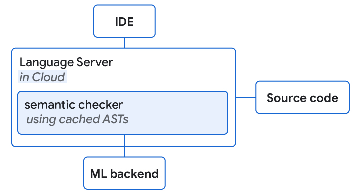 |
| Language servers with access to source code and the ML backend are collocated on the cloud. They both perform semantic checking of ML completion suggestions. |
Results
With 10k+ Google-internal developers using the completion setup in their IDE, we measured a user acceptance rate of 25-34%. We determined that the transformer-based hybrid semantic ML code completion completes >3% of code, while reducing the coding iteration time for Googlers by 6% (at a 90% confidence level). The size of the shift corresponds to typical effects observed for transformational features (e.g., key framework) that typically affect only a subpopulation, whereas ML has the potential to generalize for most major languages and engineers.
| Fraction of all code added by ML | 2.6% |
| Reduction in coding iteration duration | 6% |
| Reduction in number of context switches | 7% |
| Acceptance rate (for suggestions visible for >750ms) | 25% |
| Average characters per accept | 21 |
| Key metrics for single-line code completion measured in production for 10k+ Google-internal developers using it in their daily development across eight languages. | ||||
| Fraction of all code added by ML (with >1 line in suggestion) | 0.6% |
| Average characters per accept | 73 |
| Acceptance rate (for suggestions visible for >750ms) | 34% |
| Key metrics for multi-line code completion measured in production for 5k+ Google-internal developers using it in their daily development across eight languages. | ||||
Providing Long Completions while Exploring APIs
We also tightly integrated the semantic completion with full line completion. When the dropdown with semantic single token completions appears, we display inline the single-line completions returned from the ML model. The latter represent a continuation of the item that is the focus of the dropdown. For example, if a user looks at possible methods of an API, the inline full line completions show the full method invocation also containing all parameters of the invocation.
 |
| Integrated full line completions by ML continuing the semantic dropdown completion that is in focus. |
 |
| Suggestions of multiple line completions by ML. |
Conclusion and Future Work
We demonstrate how the combination of rule-based semantic engines and large language models can be used to significantly improve developer productivity with better code completion. As a next step, we want to utilize SEs further, by providing extra information to ML models at inference time. One example can be for long predictions to go back and forth between the ML and the SE, where the SE iteratively checks correctness and offers all possible continuations to the ML model. When adding new features powered by ML, we want to be mindful to go beyond just “smart” results, but ensure a positive impact on productivity.
Acknowledgements
This research is the outcome of a two-year collaboration between Google Core and Google Research, Brain Team. Special thanks to Marc Rasi, Yurun Shen, Vlad Pchelin, Charles Sutton, Varun Godbole, Jacob Austin, Danny Tarlow, Benjamin Lee, Satish Chandra, Ksenia Korovina, Stanislav Pyatykh, Cristopher Claeys, Petros Maniatis, Evgeny Gryaznov, Pavel Sychev, Chris Gorgolewski, Kristof Molnar, Alberto Elizondo, Ambar Murillo, Dominik Schulz, David Tattersall, Rishabh Singh, Manzil Zaheer, Ted Ying, Juanjo Carin, Alexander Froemmgen and Marcus Revaj for their contributions.
Tiny cars and big talent show Canadian policymakers the power of machine learning
In the end, it came down to 213 thousandths of a second! That was the difference between the two best times in the finale of the first AWS AWS DeepRacer Student Wildcard event hosted in Ottawa, Canada this May.
I watched in awe as 13 students competed in a live wildcard race for the AWS DeepRacer Student League, the first global autonomous racing league for students offering educational material and resources to get hands on and start with machine learning (ML).
Students hit the starting line to put their ML skills to the test in Canada’s capital where members of parliament cheered them on, including Parliamentary Secretary for Innovation, Science and Economic Development, Andy Fillmore. Daphne Hong, a fourth-year engineering student at the University of Calgary, won the race with a lap time of 11:167 seconds. Not far behind were Nixon Chan from University of Waterloo and Vijayraj Kharod from Toronto Metropolitan University.
Daphne was victorious after battling nerves earlier in the day when she took practice runs as she struggled turning the corners and quickly adjusted her model. “After seeing how the physical track did compared to the virtual one throughout the day, I was able to make some adjustments and overcome those corners and round them as I intended, so I’m super, super happy about that,” said a beaming Daphne after being presented with her championship trophy.
Daphne also received a $1,000 Amazon Canada Gift Card, while the second and third place racers — Nixon Chan and Vijayraj Kharod — got trophies and $500 gift cards. The top two contestants now have a chance to race virtually in the AWS DeepRacer Student League finale in October. “The whole experience feels like a win for me,” said DeepRacer participant Connor Hunszinger from the University of Alberta.
The event not only highlighted the importance of machine learning education to Canadian policymakers, but also made clear that these young Canadians could be poised to do great things with their ML skills.
The road to the Ottawa Wildcard
This Ottawa race is one of several wildcard events taking place around the world this year as part of the AWS DeepRacer Student League to bring students together to compete live in person. The top two finalists in each Wildcard race will have the opportunity to compete in the AWS DeepRacer Student League finale, with a chance of winning up to $5,000 USD towards their tuition. The top three racers from the student league finale in October will advance to the global AWS DeepRacer League Championship held at AWS re:Invent in Las Vegas this December.
Students who raced in Ottawa began their journey this March when they competed in the global AWS DeepRacer Student League by submitting their model to the virtual 3D simulation environment and posting times to the leaderboard. From the student league, the top student racers across Canada were selected to compete in the wildcard event. Students trained their models in preparation for the event through the virtual environment and then applied their ML models for the first time on a physical track in Ottawa. Each student competitor was given one three-minute attempt to complete their fastest lap with only the speed of the car being controlled.
“Honestly, I don’t really consider my peers here my competitors. I loved being able to work with them. It seems more like a friendly, supportive and collaborative environment. We were always cheering each other on,” says Daphne Hong, AWS DeepRacer Student League Canada Wildcard winner. “This event is great because it allows people who don’t really have that much AI or ML experience to learn more about the industry and see it live with these cars. I want to share my findings and my knowledge with those around me, those in my community and spread the word about ML and AI.”
Building access to machine learning in Canada
Machine learning talent is in hot demand, making up a large portion of AI job postings in Canada. The Canadian economy needs people with the skills recently on display at the DeepRacer event, and Canadian policymakers are intent on building an AI talent pool.
According to the World Economic Forum, 58 million jobs will be created by the growth of machine learning in the next few years, but right now, there are only 300,000 engineers with the relevant training to build and deploy ML models.
That means organizations of all types must not only train their existing workers with ML skills, but also invest in training programs and solutions to develop those capabilities for future workers. AWS is doing its part with a multitude of products for learners of all levels.
- AWS Artificial Intelligence and Machine Learning Scholarship, a $10 million education and scholarship program, aimed at preparing underserved and underrepresented students in tech globally for careers in the space.
- AWS DeepRacer, the world’s first global autonomous racing league, open to developers globally to get started in ML with a 1/18th scale race car driven by reinforcement learning. Developers can compete in the global racing league for prizes and rewards.
- AWS DeepRacer Student, a version of AWS DeepRacer open to students 16 years and older globally with free access to 20 hours of ML educational content and 10 hours of compute resources for model training monthly at no cost. Participants can compete in the global racing league exclusively for students to win scholarships and prizes.
- Machine Learning University, self service ML training courses with learn at your own pace educational content built by Amazon’s ML scientists.
Cloud computing makes access to machine learning technology a lot easier, faster — and fun, if the AWS DeepRacer Student League Wildcard event was any indication. The race was created by AWS, as an enjoyable, hands-on way to make ML more widely accessible to anyone interested in the technology.
Get started with your machine learning journey and take part in the AWS DeepRacer Student league today for your chance to wins prizes and glory.
About the author
 Nicole Foster is Director of AWS Global AI/ML and Canada Public Policy at Amazon, where she leads the direction and strategy of artificial intelligence public policy for Amazon Web Services (AWS) around the world as well as the company’s public policy efforts in support of the AWS business in Canada. In this role, she focuses on issues related to emerging technology, digital modernization, cloud computing, cyber security, data protection and privacy, government procurement, economic development, skilled immigration, workforce development, and renewable energy policy.
Predict shipment ETA with no-code machine learning using Amazon SageMaker Canvas
Logistics and transportation companies track ETA (estimated time of arrival), which is a key metric for their business. Their downstream supply chain activities are planned based on this metric. However, delays often occur, and the ETA might differ from the product’s or shipment’s actual time of arrival (ATA), for instance due to shipping distance or carrier-related or weather-related issues. This impacts the entire supply chain, in many instances reducing productivity and increasing waste and inefficiencies. Predicting the exact day a product arrives to a customer is challenging because it depends on various factors such as order type, carrier, origin, and distance.
Analysts working in the logistics and transportation industry have domain expertise and knowledge of shipping and logistics attributes. However, they need to be able to generate accurate shipment ETA forecasts for efficient business operations. They need an intuitive, easy-to-use, no-code capability to create machine learning (ML) models for predicting shipping ETA forecasts.
To help achieve the agility and effectiveness that business analysts seek, we launched Amazon SageMaker Canvas, a no-code ML solution that helps companies accelerate solutions to business problems quickly and easily. SageMaker Canvas provides business analysts with a visual point-and-click interface that allows you to build models and generate accurate ML predictions on your own—without requiring any ML experience or having to write a single line of code.
In this post, we show how to use SageMaker Canvas to predict shipment ETAs.
Solution overview
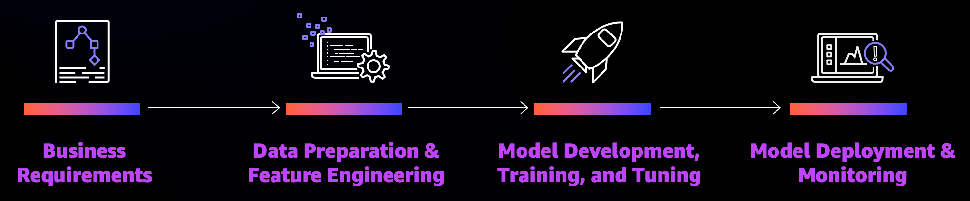
Although ML development is a complex and iterative process, we can generalize an ML workflow into business requirements analysis, data preparation, model development, and model deployment stages.
SageMaker Canvas abstracts the complexities of data preparation and model development, so you can focus on delivering value to your business by drawing insights from your data without a deep knowledge of the data science domain. The following architecture diagram highlights the components in a no-code or low-code solution.
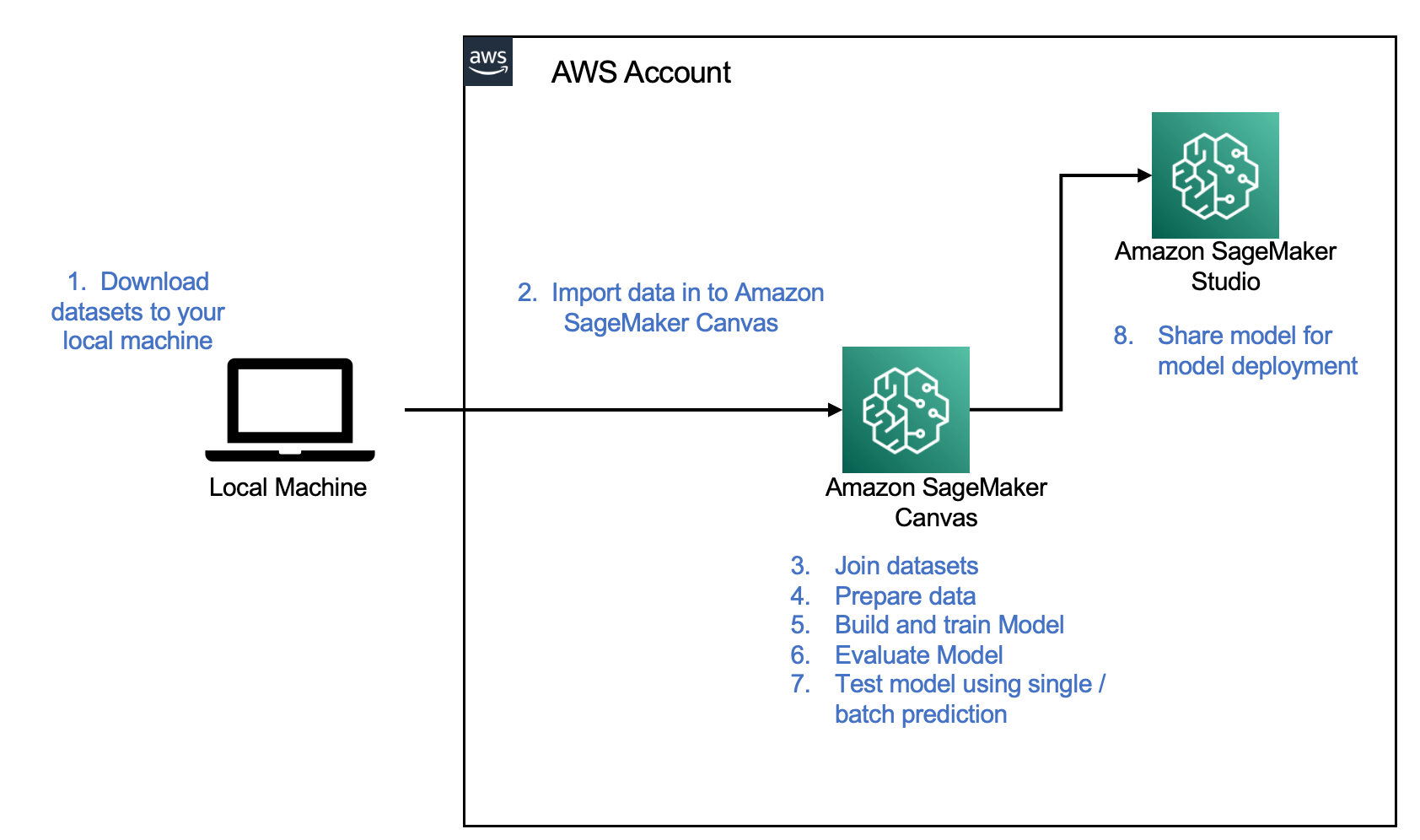
The following are the steps as outlined in the architecture:
- Download the dataset to your local machine.
- Import the data into SageMaker Canvas.
- Join your datasets.
- Prepare the data.
- Build and train your model.
- Evaluate the model.
- Test the model.
- Share the model for deployment.
Let’s assume you’re a business analyst assigned to the product shipment tracking team of a large logistics and transportation organization. Your shipment tracking team has asked you to assist in predicting the shipment ETA. They have provided you with a historical dataset that contains characteristics tied to different products and their respective ETA, and want you to predict the ETA for products that will be shipped in the future.
We use SageMaker Canvas to perform the following steps:
- Import our sample datasets.
- Join the datasets.
- Train and build the predictive machine maintenance model.
- Analyze the model results.
- Test predictions against the model.
Dataset overview
We use two datasets (shipping logs and product description) in CSV format, which contain shipping log information and certain characteristics of a product, respectively.
The ShippingLogs dataset contains the complete shipping data for all products delivered, including estimated time shipping priority, carrier, and origin. It has approximately 10,000 rows and 12 feature columns. The following table summarizes the data schema.
ActualShippingDays |
Number of days it took to deliver the shipment |
Carrier |
Carrier used for shipment |
YShippingDistance |
Distance of shipment on the Y-axis |
XShippingDistance |
Distance of shipment on the X-axis |
ExpectedShippingDays |
Expected days for shipment |
InBulkOrder |
Is it a bulk order |
ShippingOrigin |
Origin of shipment |
OrderDate |
Date when the order was placed |
OrderID |
Order ID |
ShippingPriority |
Priority of shipping |
OnTimeDelivery |
Whether the shipment was delivered on time |
ProductId |
Product ID |
The ProductDescription dataset contains metadata information of the product that is being shipped in the order. This dataset has approximately 10,000 rows and 5 feature columns. The following table summarizes the data schema.
ComputerBrand |
Brand of the computer |
ComputeModel |
Model of the computer |
ScreeenSize |
Screen size of the computer |
PackageWeight |
Package weight |
ProductID |
Product ID |
Prerequisites
An IT administrator with an AWS account with appropriate permissions must complete the following prerequisites:
- Deploy an Amazon SageMaker domain. For instructions, see Onboard to Amazon SageMaker Domain.
- Launch SageMaker Canvas. For instructions, see Setting up and managing Amazon SageMaker Canvas (for IT administrators).
- Configure cross-origin resource sharing (CORS) policies in Amazon Simple Storage Service (Amazon S3) for SageMaker Canvas to enable the upload option from local disk. For instructions, see Give your users the ability to upload local files.
Import the dataset
First, download the datasets (shipping logs and product description) and review the files to make sure all the data is there.
SageMaker Canvas provides several sample datasets in your application to help you get started. To learn more about the SageMaker-provided sample datasets you can experiment with, see Use sample datasets. If you use the sample datasets (canvas-sample-shipping-logs.csv and canvas-sample-product-descriptions.csv) available within SageMaker Canvas, you don’t have to import the shipping logs and product description datasets.
You can import data from different data sources into SageMaker Canvas. If you plan to use your own dataset, follow the steps in Importing data in Amazon SageMaker Canvas.
For this post, we use the full shipping logs and product description datasets that we downloaded.
- Sign in to the AWS Management Console, using an account with the appropriate permissions to access SageMaker Canvas.
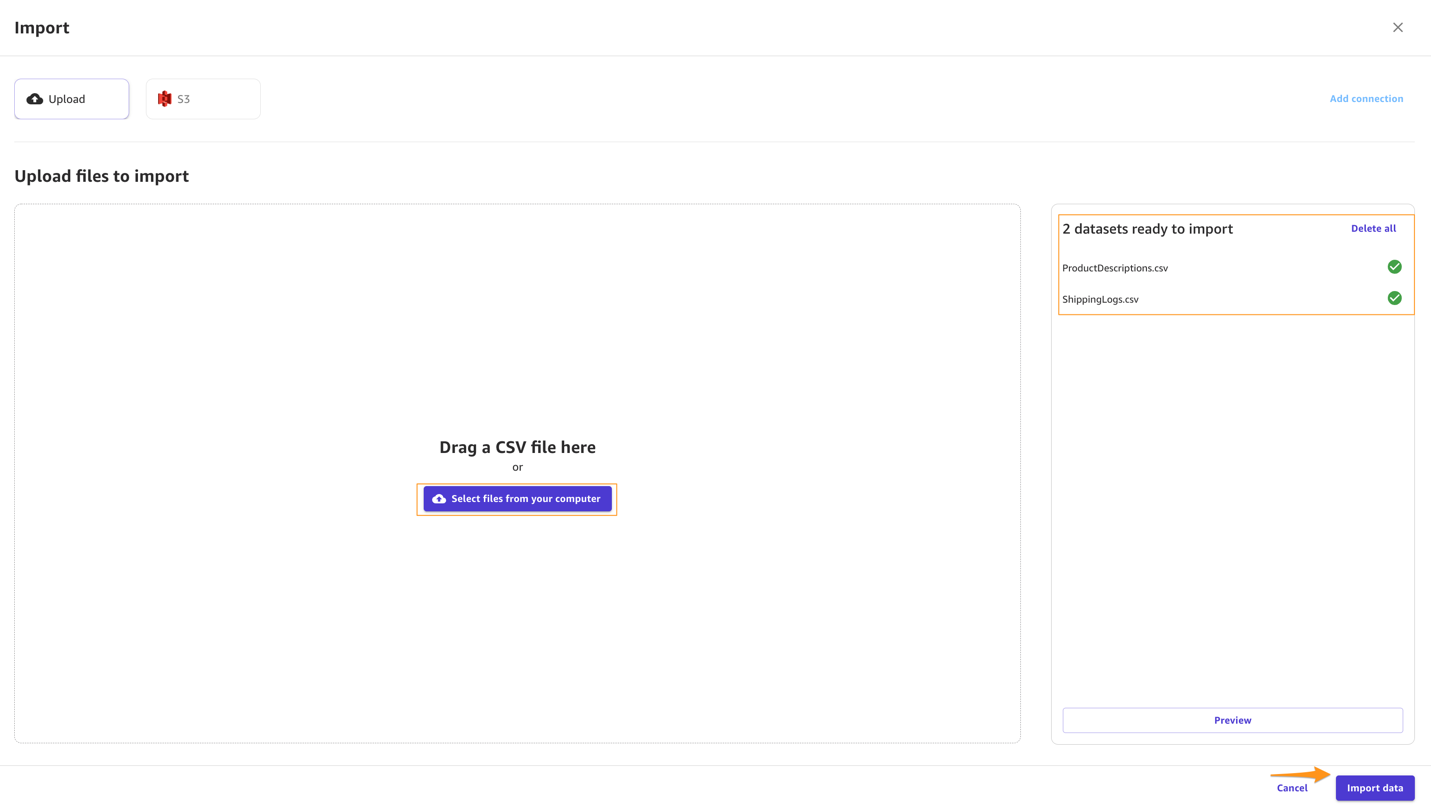
- On the SageMaker Canvas console, choose Import.
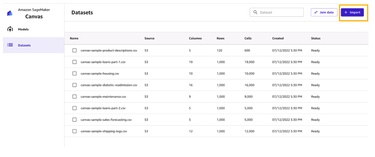
- Choose Upload and select the files
ShippingLogs.csvandProductDescriptions.csv. - Choose Import data to upload the files to SageMaker Canvas.
Create a consolidated dataset
Next, let’s join the two datasets.
- Choose Join data.

- Drag and drop
ShippingLogs.csvandProductDescriptions.csvfrom the left pane under Datasets to the right pane.
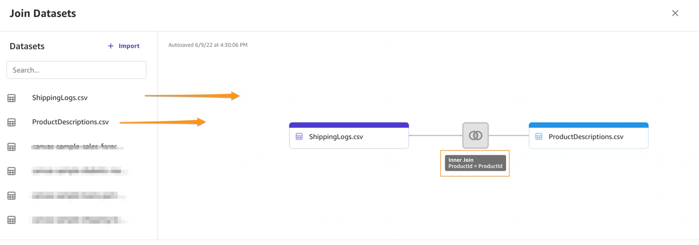 The two datasets are joined using
 ProductIDas the inner join reference. - Choose Import and enter a name for the new joined dataset.
- Choose Import data.

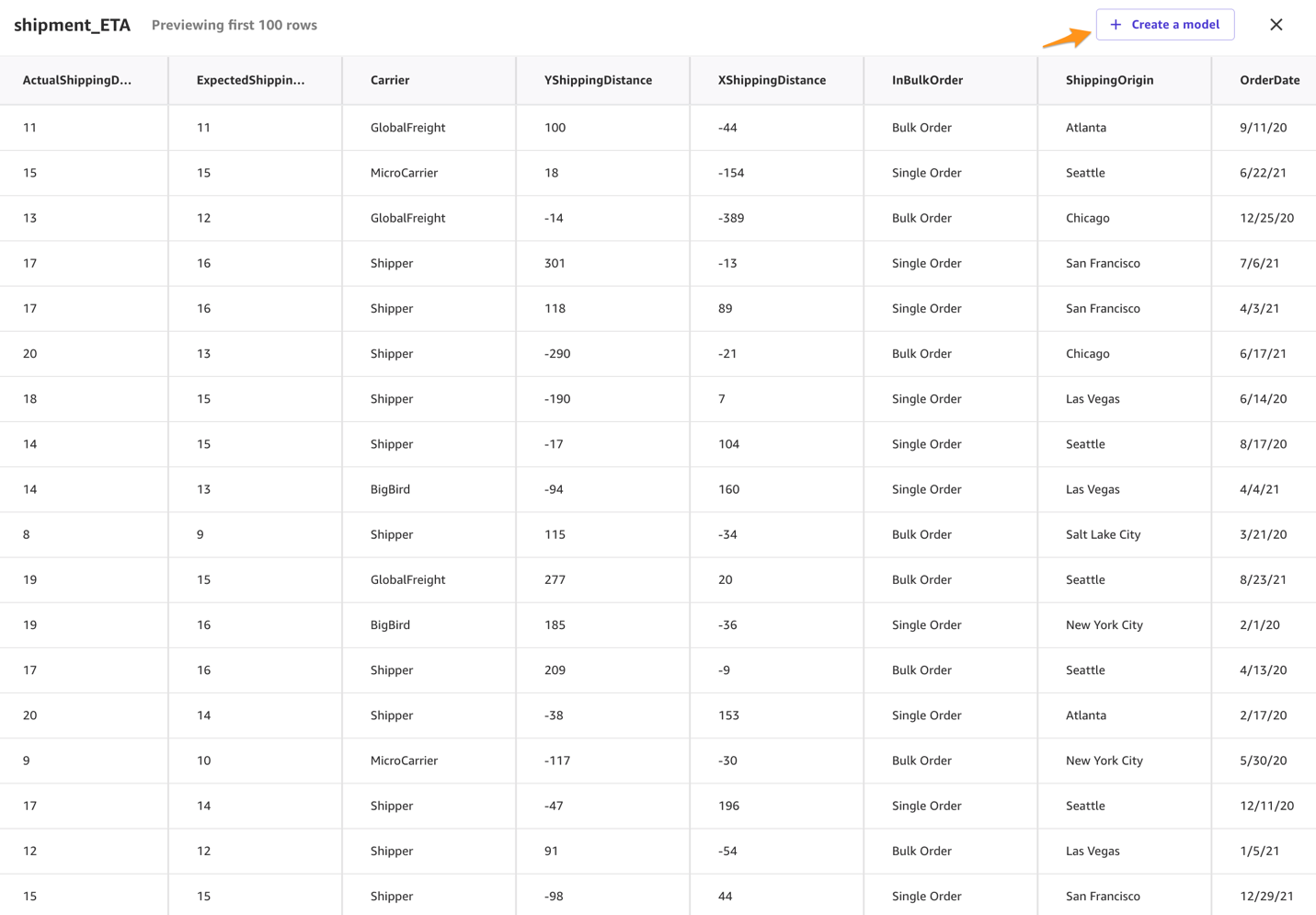
You can choose the new dataset to preview its contents.
After you review the dataset, you can create your model.
Build and train model
To build and train your model, complete the following steps:
- For Model name, enter
ShippingForecast. - Choose Create.
 In the Model view, you can see four tabs, which correspond to the four steps to create a model and use it to generate predictions: Select, Build, Analyze, and Predict.
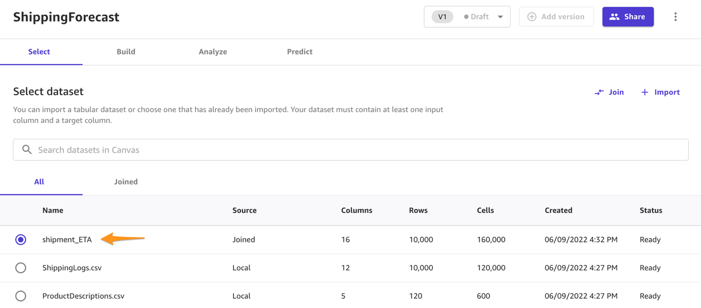
 - On the Select tab, select the
ConsolidatedShippingDatayou created earlier.You can see that this dataset comes from Amazon S3, has 12 columns, and 10,000 rows. - Choose Select dataset.
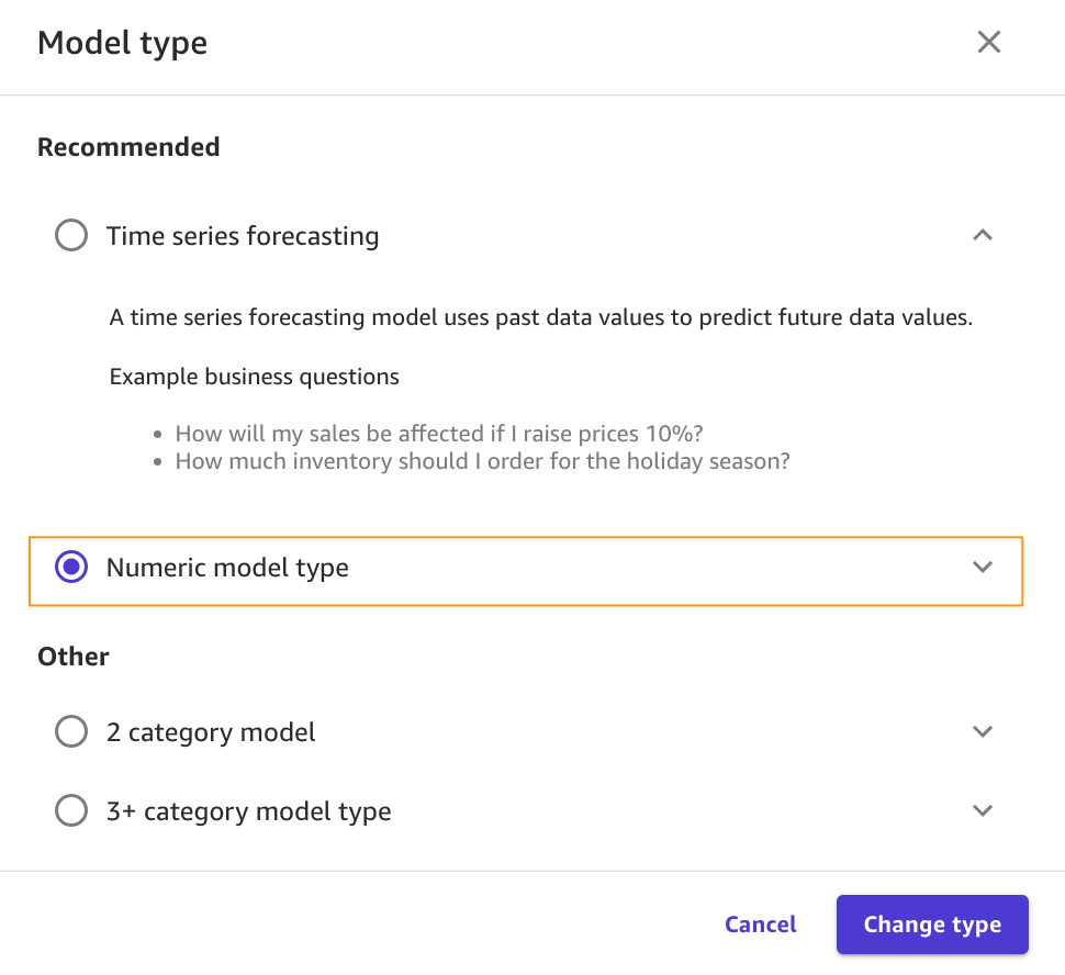
SageMaker Canvas automatically moves to the Build tab. - On the Build tab, choose the target column, in our case
ActualShippingDays.
Because we’re interested in how many days it will take for the goods to arrive for the customer, SageMaker Canvas automatically detects that this is a numeric prediction problem (also known as regression). Regression estimates the values of a dependent target variable based on one or more other variables or attributes that are correlated with it.Because we also have a column with time series data (OrderDate), SageMaker Canvas may interpret this as a time series forecast model type. - Before advancing, make sure that the model type is indeed Numeric model type; if that’s not the case, you can select it with the Change type option.
Data preparation
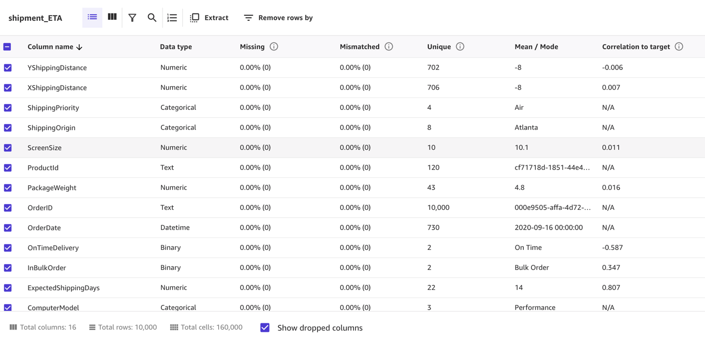
In the bottom half of the page, you can look at some of the statistics of the dataset, including missing and mismatched values, unique values, and mean and median values.
Column view provides you with the listing of all columns, their data types, and their basic statistics, including missing and mismatched values, unique values, and mean and median values. This can help you devise a strategy to handle missing values in the datasets.
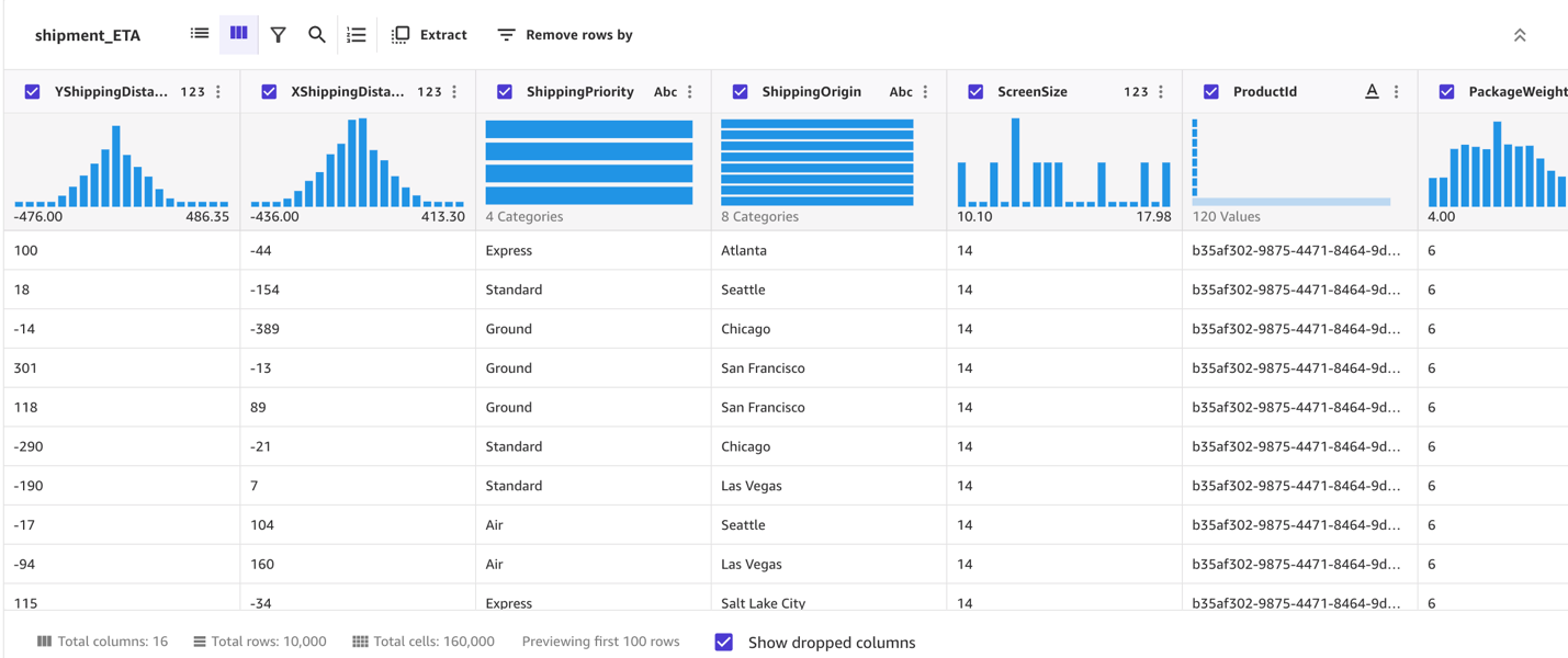
Grid view provides you with a graphical distribution of values for each column and the sample data. You can start inferring relevant columns for the training the model.
Let’s preview the model to see the estimated RMSE (root mean squared error) for this numeric prediction.
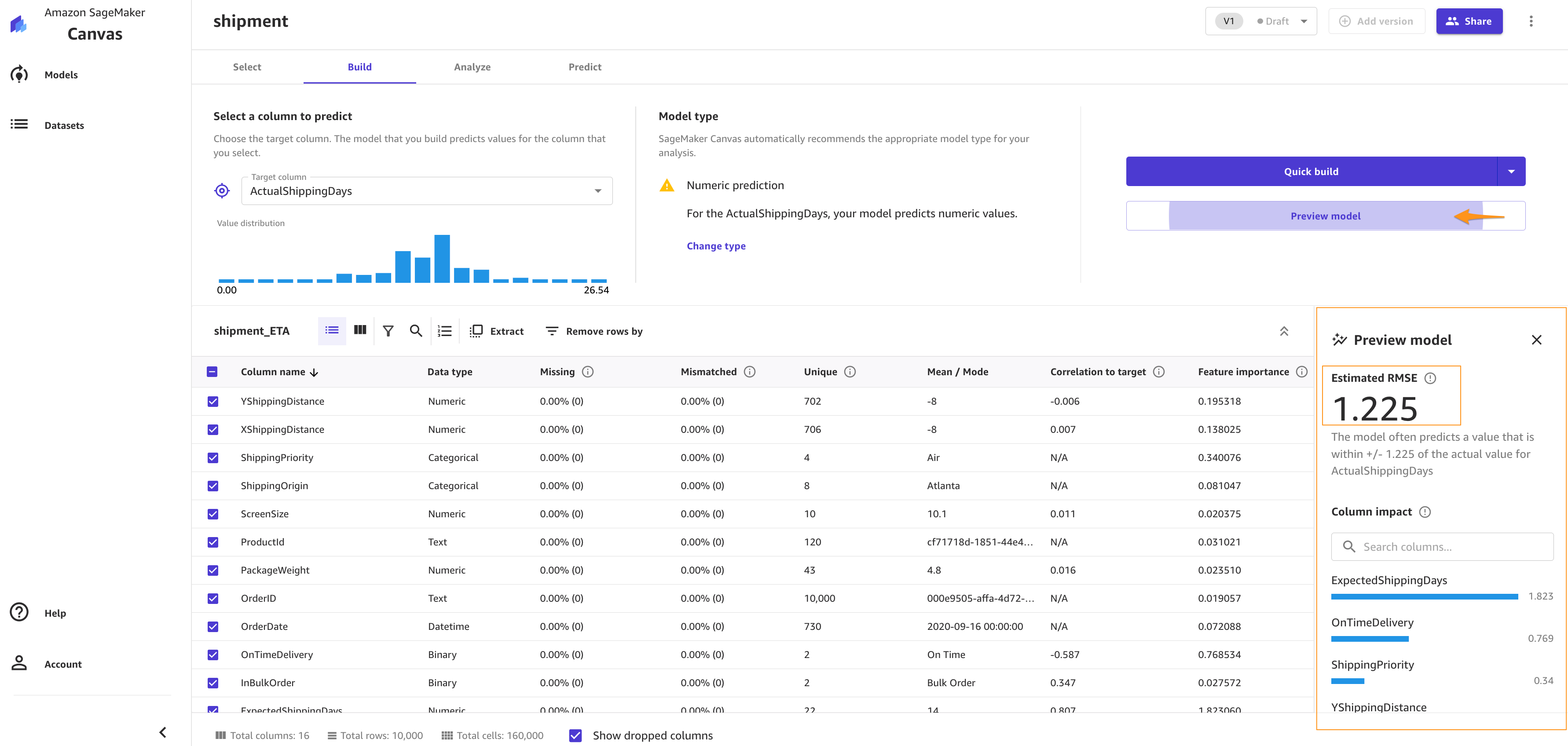
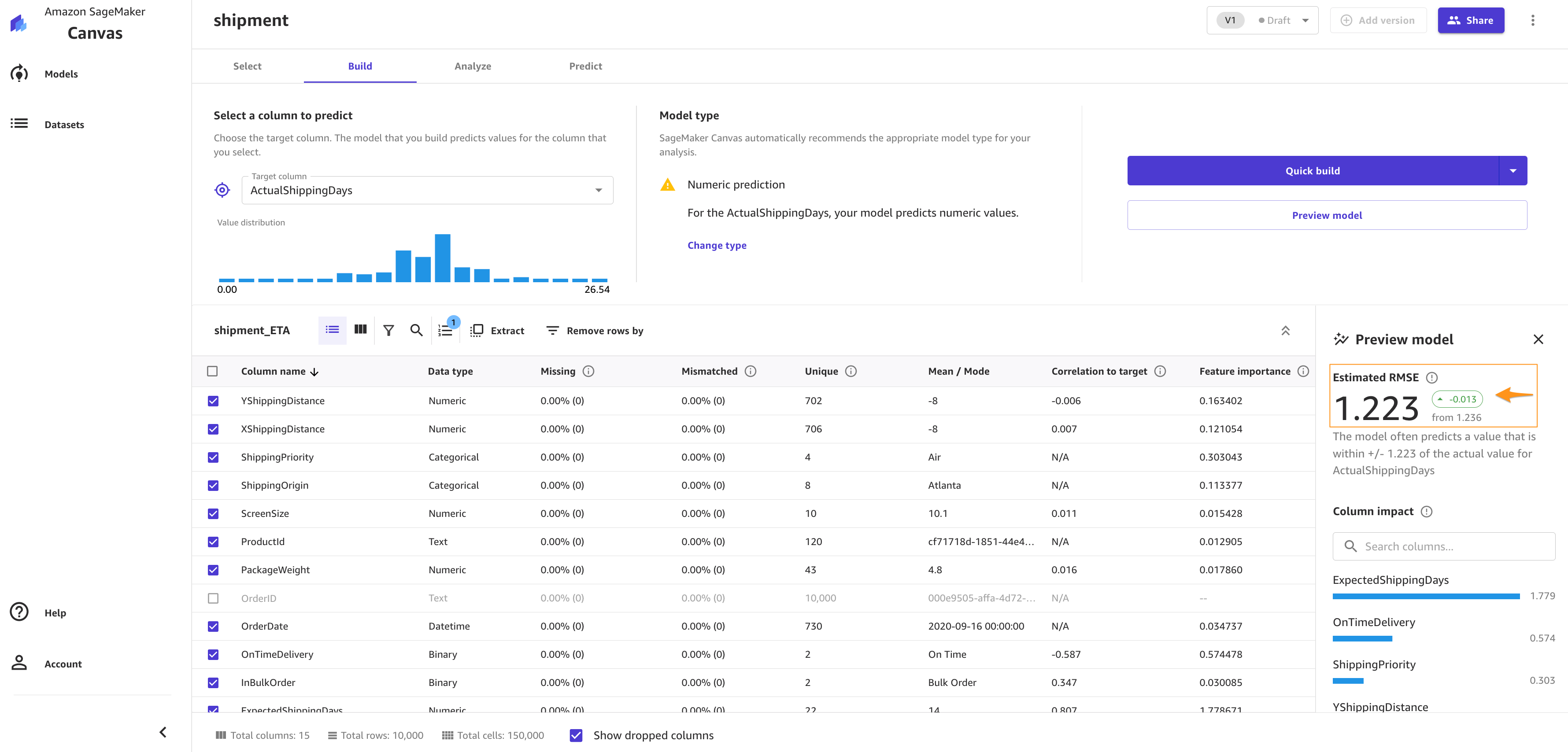
You can also drop some of the columns, if you don’t want to use them for the prediction, by simply deselecting them. For this post, we deselect the order*_**id* column. Because it’s a primary key, it doesn’t have valuable information, and so doesn’t add value to the model training process.
You can choose Preview model to get insights on feature importance and iterate the model quickly. We also see the RMSE is now 1.223, which is improved from 1.225. The lower the RMSE, the better a given model is able to fit a dataset.
From our exploratory data analysis, we can see that the dataset doesn’t have a lot of missing values. Therefore, we don’t have to handle missing values. If you see a lot of missing values for your features, you can filter the missing values.
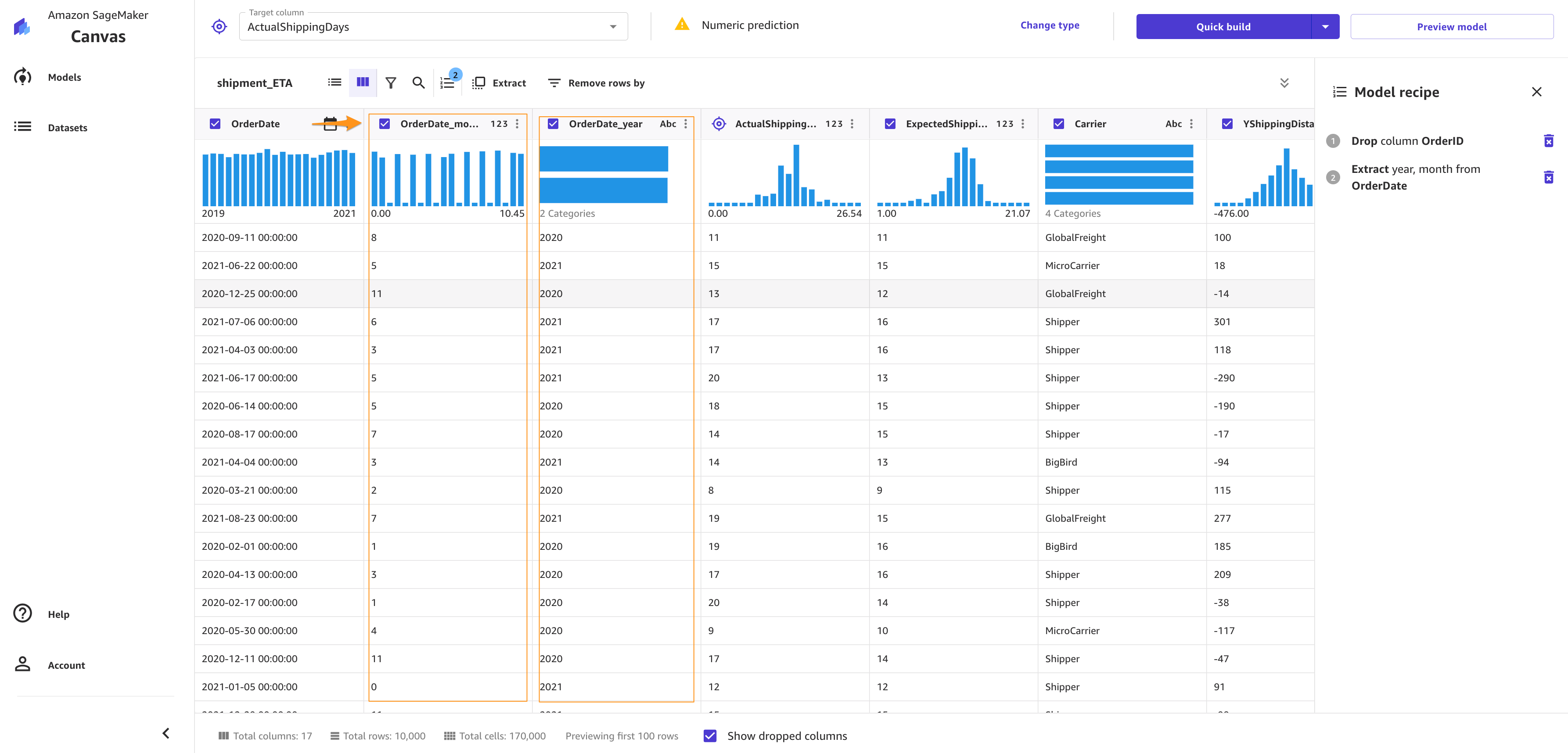
To extract more insights, you can proceed with a datetime extraction. With the datetime extraction transform, you can extract values from a datetime column to a separate column.
To perform a datetime extraction, complete the following steps:
- On the Build tab of the SageMaker Canvas application, choose Extract.
- Choose the column from which you want to extract values (for this post,
OrderDate). - For Value, choose one or more values to extract from the column. For this post, we choose Year and Month.The values you can extract from a timestamp column are Year, Month, Day, Hour, Week of year, Day of year, and Quarter.
- Choose Add to add the transform to the model recipe.

SageMaker Canvas creates a new column in the dataset for each of the values you extract.
Model training
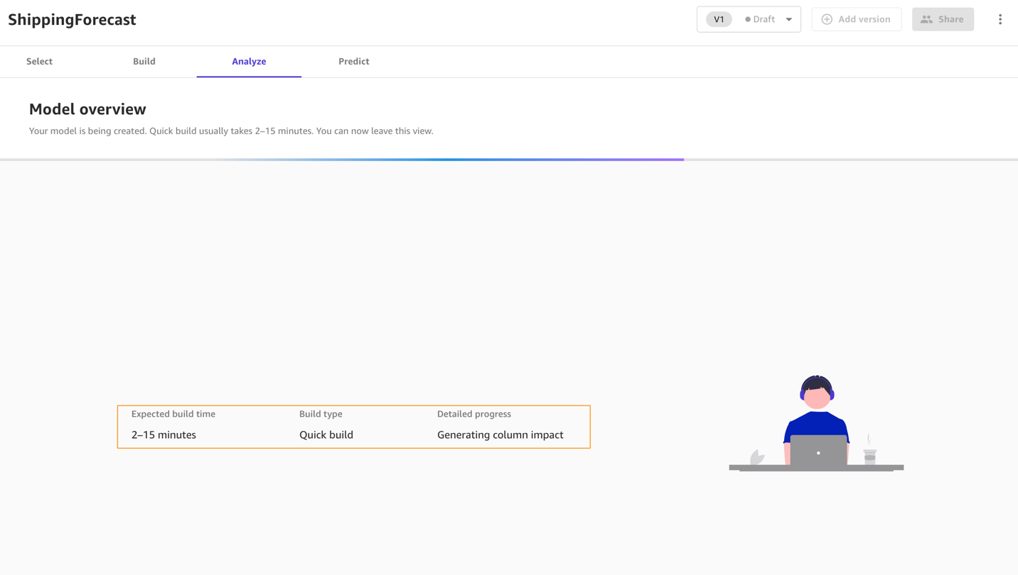
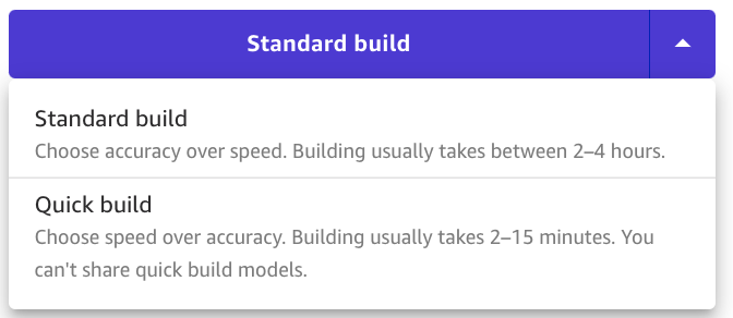
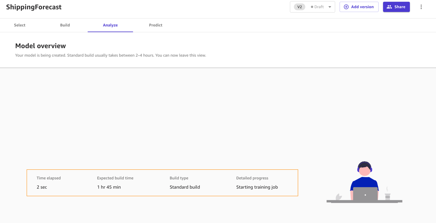
It’s time to finally train the model! Before building a complete model, it’s a good practice to have a general idea about the performances that our model will have by training a quick model. A quick model trains fewer combinations of models and hyperparameters in order to prioritize speed over accuracy. This is helpful in cases like ours where we want to prove the value of training an ML model for our use case. Note that the quick build option isn’t available for models bigger than 50,000 rows.
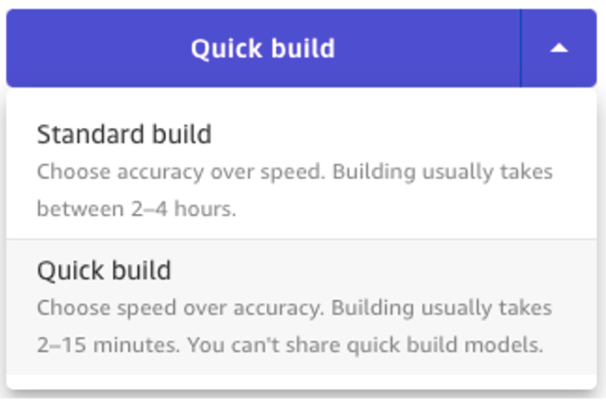
Now we wait anywhere from 2–15 minutes for the quick build to finish training our model.
Evaluate model performance
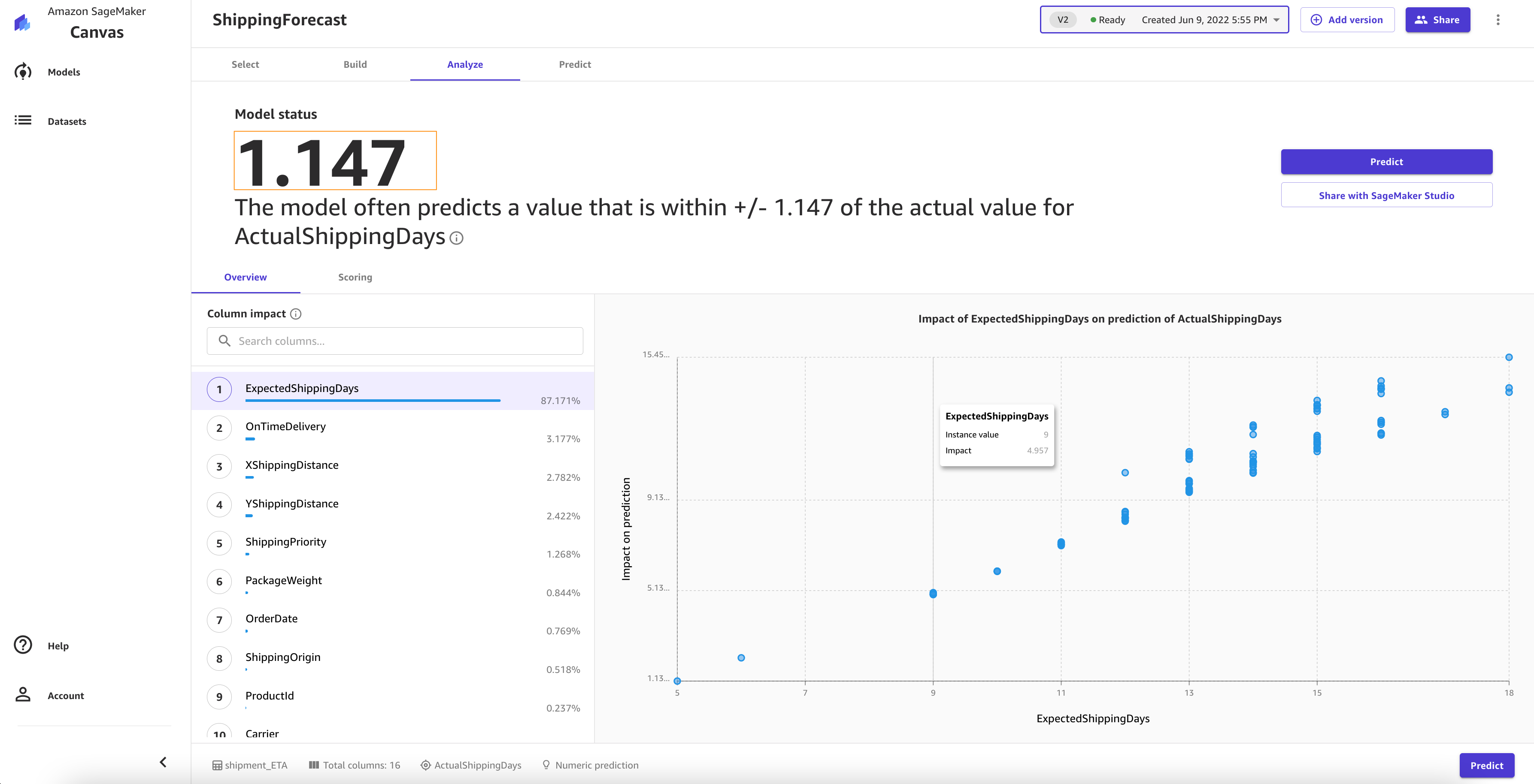
When training is complete, SageMaker Canvas automatically moves to the Analyze tab to show us the results of our quick training, as shown in the following screenshot.
You may experience slightly different values. This is expected. Machine learning introduces some variation in the process of training models, which can lead to different results for different builds.
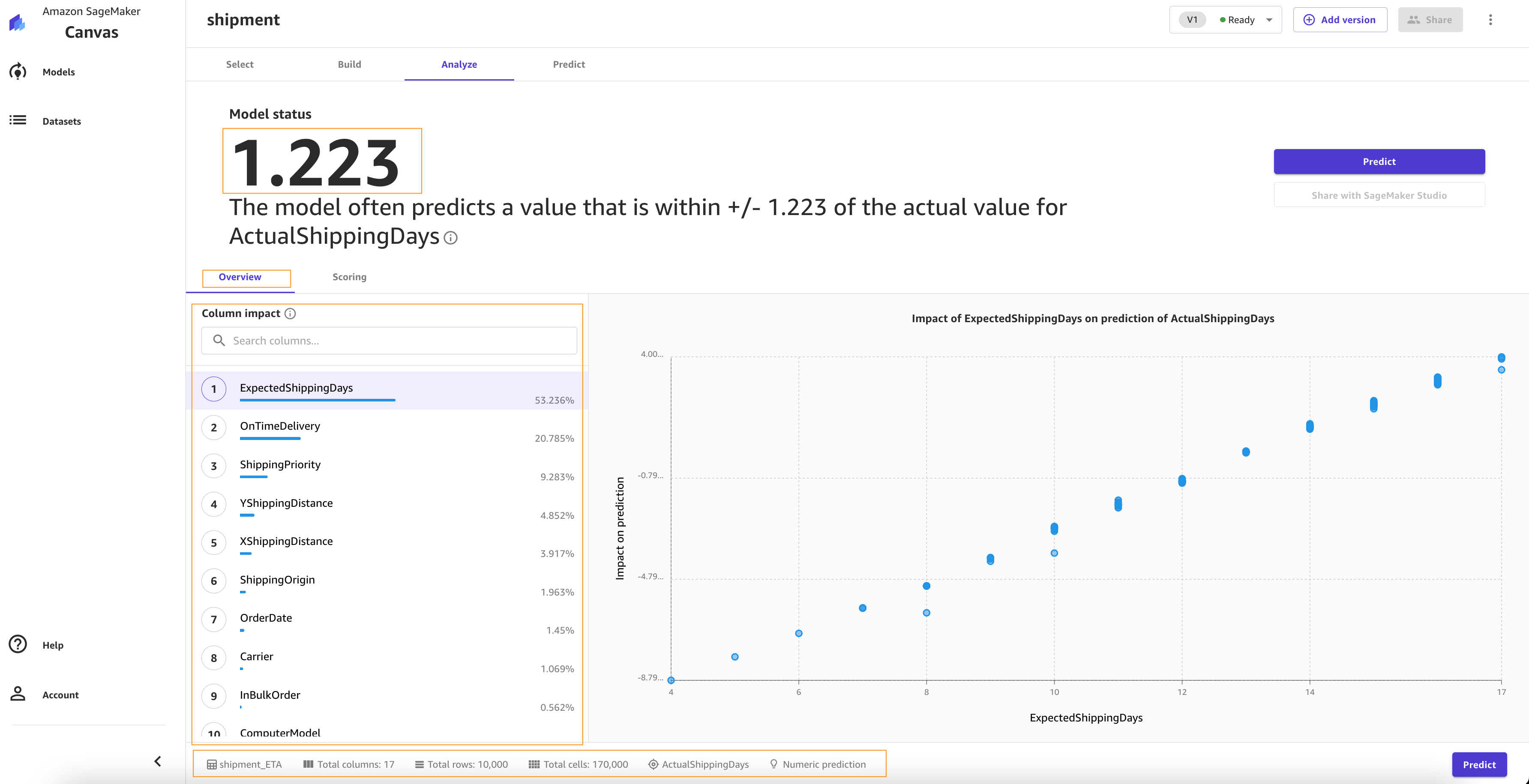
Let’s focus on the Overview tab. This tab shows you the column impact, or the estimated importance of each column in predicting the target column. In this example, the ExpectedShippingDays column has the most significant impact in our predictions.
On the Scoring tab, you can see a plot representing the best fit regression line for ActualshippingDays. On average, the model prediction has a difference of +/- 0.7 from the actual value of ActualShippingDays. The Scoring section for numeric prediction shows a line to indicate the model’s predicted value in relation to the data used to make predictions. The values of the numeric prediction are often +/- the RMSE value. The value that the model predicts is often within the range of the RMSE. The width of the purple band around the line indicates the RMSE range. The predicted values often fall within the range.
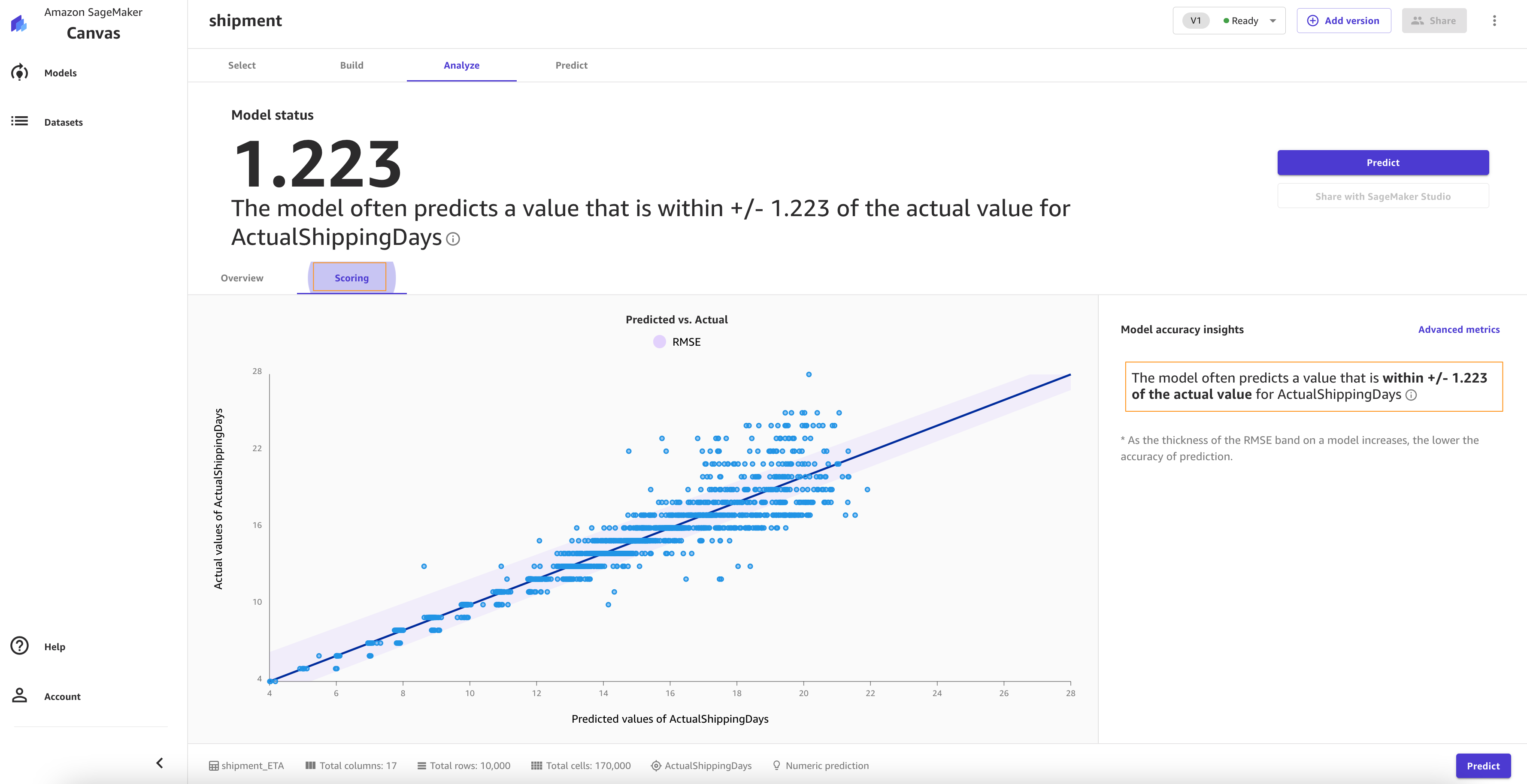
As the thickness of the RMSE band on a model increases, the accuracy of the prediction decreases. As you can see, the model predicts with high accuracy to begin with (lean band) and as the value of actualshippingdays increases (17–22), the band becomes thicker, indicating lower accuracy.
The Advanced metrics section contains information for users that want a deeper understanding of their model performance. The metrics for numeric prediction are as follows:
- R2 – The percentage of the difference in the target column that can be explained by the input column.
- MAE – Mean absolute error. On average, the prediction for the target column is +/- {MAE} from the actual value.
- MAPE – Mean absolute percent error. On average, the prediction for the target column is +/- {MAPE} % from the actual value.
- RMSE – Root mean square error. The standard deviation of the errors.
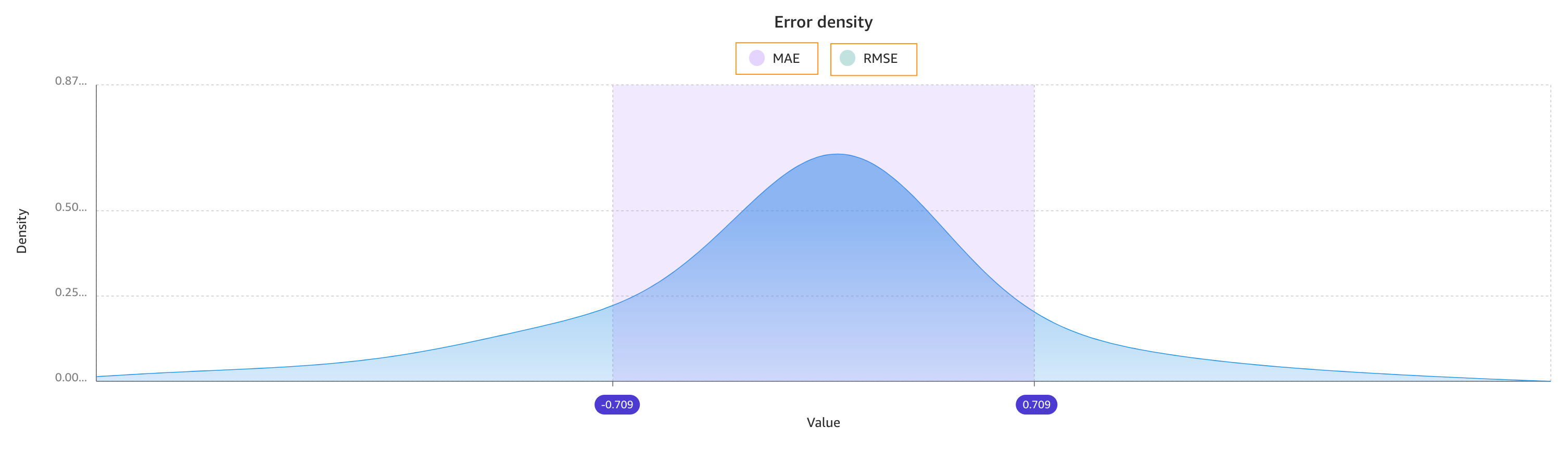
The following screenshot shows a graph of the residuals or errors. The horizontal line indicates an error of 0 or a perfect prediction. The blue dots are the errors. Their distance from the horizontal line indicates the magnitude of the errors.
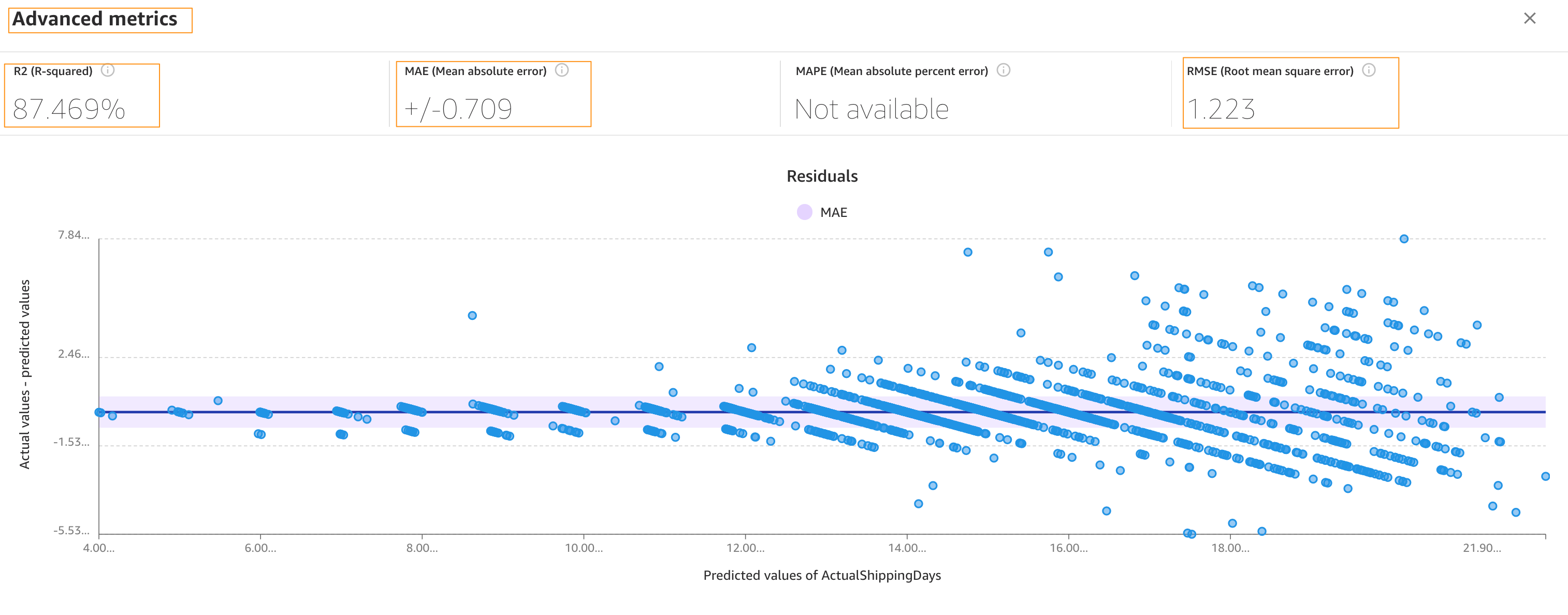
R-squared is a statistical measure of how close the data is to the fitted regression line. The higher percentage indicates that the model explains all the variability of the response data around its mean 87% of the time.
On average, the prediction for the target column is +/- 0.709 {MAE} from the actual value. This indicates that on average the model will predict the target within half a day. This is useful for planning purposes.
The model has a standard deviation (RMSE) of 1.223. As you can see, the model predicts with high accuracy to begin with (lean band) and as the value of actualshippingdays increases (17–22), the band becomes thicker, indicating lower accuracy.
The following image shows an error density plot.
You now have two options as next steps:
- You can use this model to run some predictions by choosing Predict.
- You can create a new version of this model to train with the Standard build option. This will take much longer—about 4–6 hours—but will produce more accurate results.
Because we feel confident about using this model given the performances we’ve seen, we opt to go ahead and use the model for predictions. If you weren’t confident, you could have a data scientist review the modeling SageMaker Canvas did and offer potential improvements.
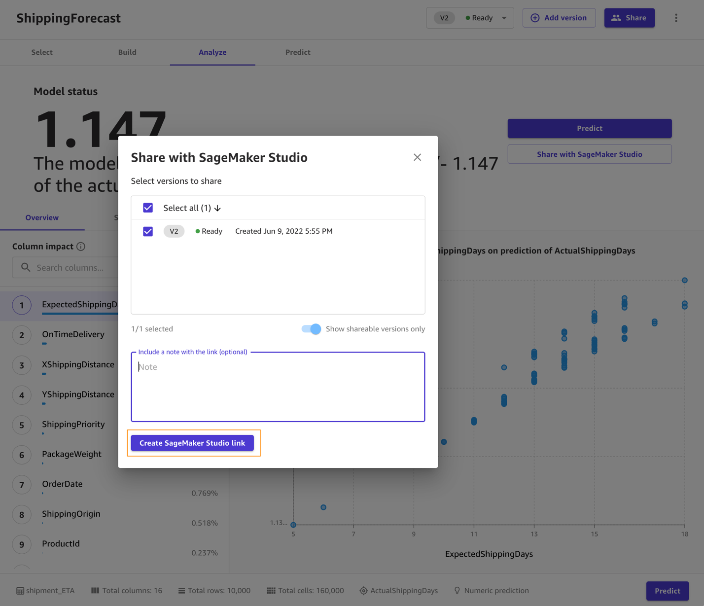
Note that training a model with the Standard build option is necessary to share the model with a data scientist with the Amazon SageMaker Studio integration.
Generate predictions
Now that the model is trained, let’s generate some predictions.
- Choose Predict on the Analyze tab, or choose the Predict tab.
- Choose Batch prediction.
- Choose Select dataset, and choose the dataset
ConsolidatedShipping.csv.
SageMaker Canvas uses this dataset to generate our predictions. Although it’s generally not a good idea not to use the same dataset for both training and testing, we’re using the same dataset for the sake of simplicity. You can also import another dataset if you desire.
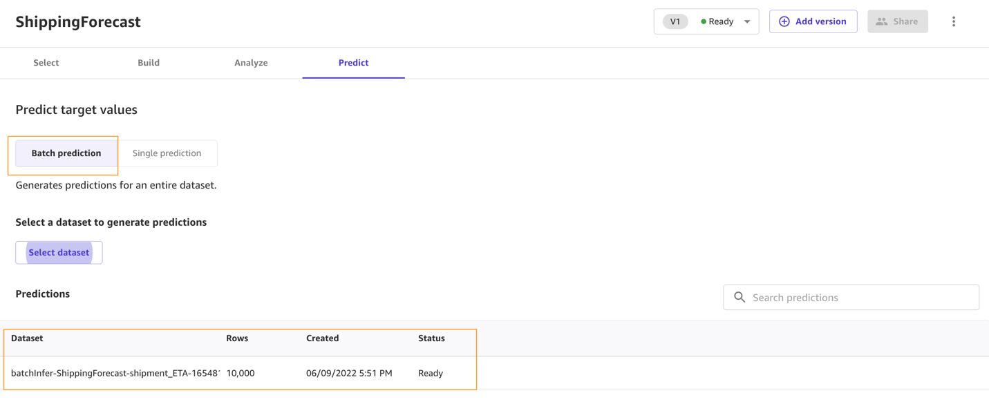
After a few seconds, the prediction is done and you can choose the eye icon to see a preview of the predictions, or choose Download to download a CSV file containing the full output.
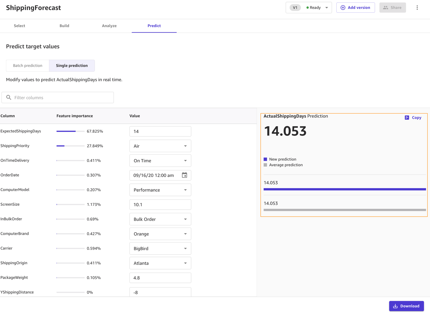
You can also choose to predict values one by one by selecting Single prediction instead of Batch prediction. SageMaker Canvas then shows you a view where you can provide the values for each feature manually and generate a prediction. This is ideal for situations like what-if scenarios—for example, how does ActualShippingDays change if the ShippingOrigin is Houston? What if we used a different carrier? What if the PackageWeight is different?
Standard build
Standard build chooses accuracy over speed. If you want to share the artifacts of the model with your data scientist and ML engineers, you may choose to create a standard build next.
First add a new version.

Then choose Standard build.
The Analyze tab shows your build progress.
When the model is complete, you can observe that the RMSE value of the standard build is 1.147, compared to 1.223 with the quick build.
After you create a standard build, you can share the model with data scientists and ML engineers for further evaluation and iteration.
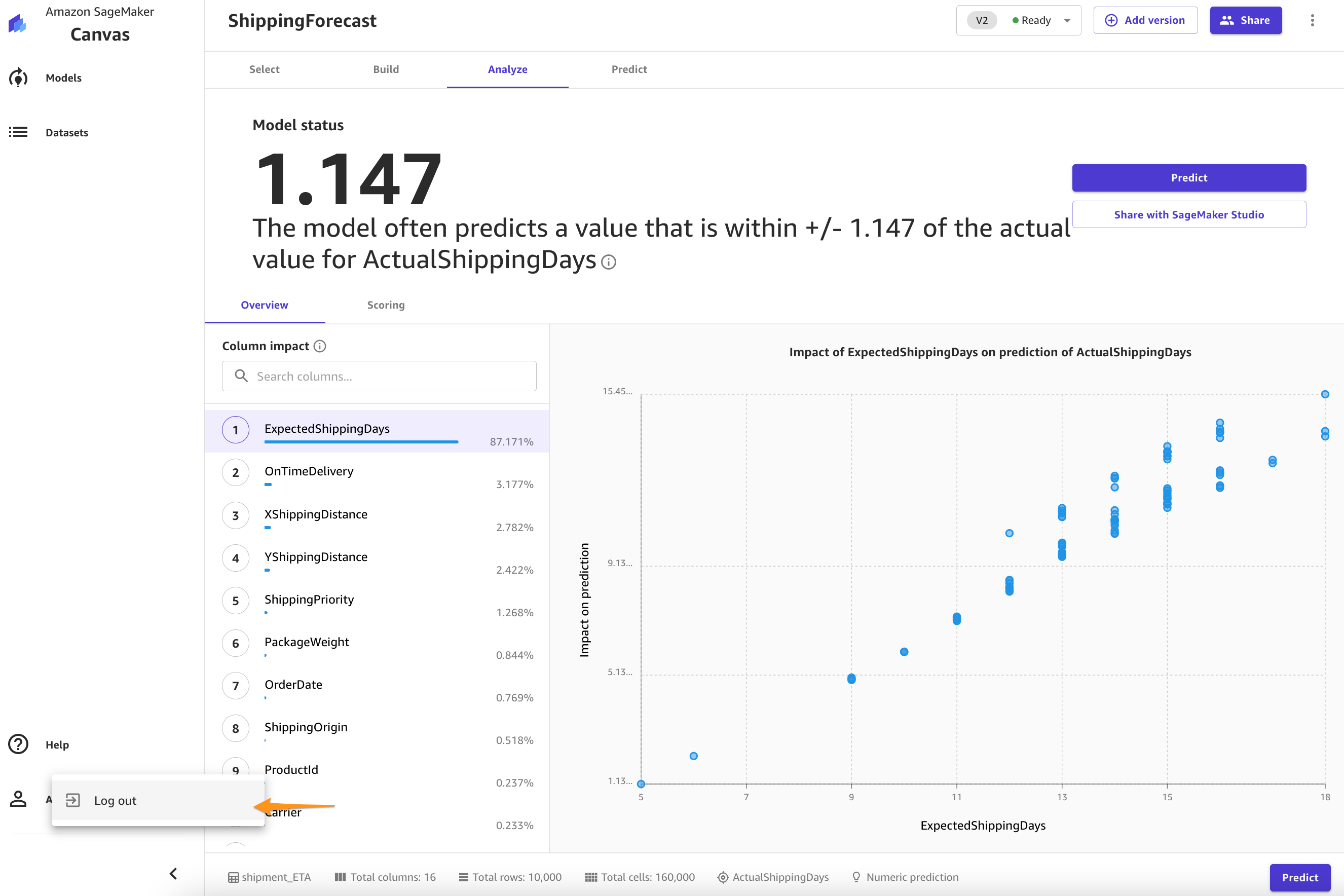
Clean up
To avoid incurring future session charges, log out of SageMaker Canvas.
Conclusion
In this post, we showed how a business analyst can create a shipment ETA prediction model with SageMaker Canvas using sample data. SageMaker Canvas allows you to create accurate ML models and generate predictions using a no-code, visual, point-and-click interface. Analysts can take this to the next level by sharing their models with data scientist colleagues. The data scientists can view the SageMaker Canvas model in Studio, where they can explore the choices SageMaker Canvas made to generate ML models, validate model results, and even take the model to production with a few clicks. This can accelerate ML-based value creation and help scale improved outcomes faster.
- To learn more about using SageMaker Canvas, see Build, Share, Deploy: how business analysts and data scientists achieve faster time-to-market using no-code ML and Amazon SageMaker Canvas.
- For more information about creating ML models with a no-code solution, see Announcing Amazon SageMaker Canvas – a Visual, No Code Machine Learning Capability for Business Analysts.
About the authors
 Rajakumar Sampathkumar is a Principal Technical Account Manager at AWS, providing customers guidance on business-technology alignment and supporting the reinvention of their cloud operation models and processes. He is passionate about the cloud and machine learning. Raj is also a machine learning specialist and works with AWS customers to design, deploy, and manage their AWS workloads and architectures.
 Meenakshisundaram Thandavarayan is a Senior AI/ML specialist with a passion to design, create and promote human-centered Data and Analytics experiences. He supports AWS Strategic customers on their transformation towards data driven organization.
What Is an Exaflop?
Computers are crunching more numbers than ever to crack the most complex problems of our time — how to cure diseases like COVID and cancer, mitigate climate change and more.
These and other grand challenges ushered computing into today’s exascale era when top performance is often measured in exaflops.
So, What’s an Exaflop?
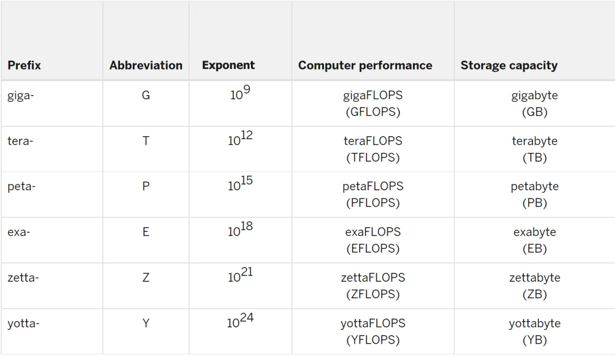
An exaflop is a measure of performance for a supercomputer that can calculate at least 1018 or one quintillion floating point operations per second.
In exaflop, the exa- prefix means a quintillion, that’s a billion billion, or one followed by 18 zeros. Similarly, an exabyte is a memory subsystem packing a quintillion bytes of data.
The “flop” in exaflop is an abbreviation for floating point operations. The rate at which a system executes a flop in seconds is measured in exaflop/s.
Floating point refers to calculations made where all the numbers are expressed with decimal points.
1,000 Petaflops = an Exaflop
The prefix peta- means 1015, or one with 15 zeros behind it. So, an exaflop is a thousand petaflops.
To get a sense of what a heady calculation an exaflop is, imagine a billion people, each holding a billion calculators. (Clearly, they’ve got big hands!)
If they all hit the equal sign at the same time, they’d execute one exaflop.
Indiana University, home to the Big Red 200 and several other supercomputers, puts it this way: To match what an exaflop computer can do in just one second, you’d have to perform one calculation every second for 31,688,765,000 years.
A Brief History of the Exaflop
For most of supercomputing’s history, a flop was a flop, a reality that’s morphing as workloads embrace AI.
People used numbers expressed in the highest of several precision formats, called double precision, as defined by the IEEE Standard for Floating Point Arithmetic. It’s dubbed double precision, or FP64, because each number in a calculation requires 64 bits, data nuggets expressed as a zero or one. By contrast, single precision uses 32 bits.
Double precision uses those 64 bits to ensure each number is accurate to a tiny fraction. It’s like saying 1.0001 + 1.0001 = 2.0002, instead of 1 + 1 = 2.
The format is a great fit for what made up the bulk of the workloads at the time — simulations of everything, from atoms to airplanes, that need to ensure their results come close to what they represent in the real world.
So, it was natural that the LINPACK benchmark, aka HPL, that measures performance on FP64 math became the default measurement in 1993, when the TOP500 list of world’s most powerful supercomputers debuted.
The Big Bang of AI
A decade ago, the computing industry heard what NVIDIA CEO Jensen Huang describes as the big bang of AI.
This powerful new form of computing started showing significant results on scientific and business applications. And it takes advantage of some very different mathematical methods.
Deep learning is not about simulating real-world objects; it’s about sifting through mountains of data to find patterns that enable fresh insights.
Its math demands high throughput, so doing many, many calculations with simplified numbers (like 1.01 instead of 1.0001) is much better than doing fewer calculations with more complex ones.
That’s why AI uses lower precision formats like FP32, FP16 and FP8. Their 32-, 16- and 8-bit numbers let users do more calculations faster.
Mixed Precision Evolves
For AI, using 64-bit numbers would be like taking your whole closet when going away for the weekend.
Finding the ideal lower-precision technique for AI is an active area of research.
For example, the first NVIDIA Tensor Core GPU, Volta, used mixed precision. It executed matrix multiplication in FP16, then accumulated the results in FP32 for higher accuracy.
Hopper Accelerates With FP8
More recently, the NVIDIA Hopper architecture debuted with a lower-precision method for training AI that’s even faster. The Hopper Transformer Engine automatically analyzes a workload, adopts FP8 whenever possible and accumulates results in FP32.
When it comes to the less compute-intensive job of inference — running AI models in production — major frameworks such as TensorFlow and PyTorch support 8-bit integer numbers for fast performance. That’s because they don’t need decimal points to do their work.
The good news is NVIDIA GPUs support all precision formats (above), so users can accelerate every workload optimally.
Last year, the IEEE P3109 committee started work on an industry standard for precision formats used in machine learning. This work could take another year or two.
Some Sims Shine at Lower Precision
While FP64 remains popular for simulations, many use lower-precision math when it delivers useful results faster.
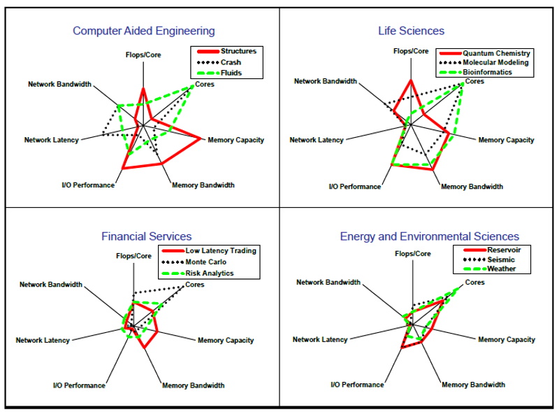
For example, researchers run in FP32 a popular simulator for car crashes, LS-Dyna from Ansys. Genomics is another field that tends to prefer lower-precision math.
In addition, many traditional simulations are starting to adopt AI for at least part of their workflows. As workloads shift towards AI, supercomputers need to support lower precision to run these emerging applications well.
Benchmarks Evolve With Workloads
Recognizing these changes, researchers including Jack Dongarra — the 2021 Turing award winner and a contributor to HPL — debuted HPL-AI in 2019. It’s a new benchmark that’s better for measuring these new workloads.
“Mixed-precision techniques have become increasingly important to improve the computing efficiency of supercomputers, both for traditional simulations with iterative refinement techniques as well as for AI applications,” Dongarra said in a 2019 blog. “Just as HPL allows benchmarking of double-precision capabilities, this new approach based on HPL allows benchmarking of mixed-precision capabilities of supercomputers at scale.”
Thomas Lippert, director of the Jülich Supercomputing Center, agreed.
“We’re using the HPL-AI benchmark because it’s a good measure of the mixed-precision work in a growing number of our AI and scientific workloads — and it reflects accurate 64-bit floating point results, too,” he said in a blog posted last year.
Today’s Exaflop Systems
In a June report, 20 supercomputer centers around the world reported their HPL-AI results, three of them delivering more than an exaflop.
One of those systems, a supercomputer at Oak Ridge National Laboratory, also exceeded an exaflop in FP64 performance on HPL.
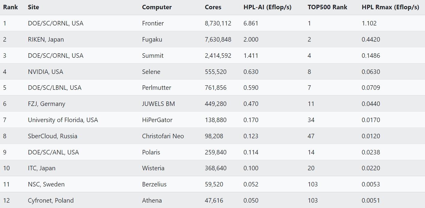
Two years ago, a very unconventional system was the first to hit an exaflop. The crowd-sourced supercomputer assembled by the Folding@home consortium passed the milestone after it put out a call for help fighting the COVID-19 pandemic and was deluged with donated time on more than a million computers.
Exaflop in Theory and Practice
Since then, many organizations have installed supercomputers that deliver more than an exaflop in theoretical peak performance. It’s worth noting that the TOP500 list reports both Rmax (actual) and Rpeak (theoretical) scores.
Rmax is simply the best performance a computer actually demonstrated.
Rpeak is a system’s top theoretical performance if everything could run at its highest possible level, something that almost never really happens. It’s typically calculated by multiplying the number of processors in a system by their clock speed, then multiplying the result by the number of floating point operations the processors can perform in one second.
So, if someone says their system can do an exaflop, consider asking if that’s using Rmax (actual) or Rpeak (theoretical).
Many Metrics in the Exaflop Age
It’s another one of the many nuances in this new exascale era.
And it’s worth noting that HPL and HPL-AI are synthetic benchmarks, meaning they measure performance on math routines, not real-world applications. Other benchmarks, like MLPerf, are based on real-world workloads.
In the end, the best measure of a system’s performance, of course, is how well it runs a user’s applications. That’s a measure not based on exaflops, but on ROI.
The post What Is an Exaflop? appeared first on NVIDIA Blog.
Preparing today for a post-quantum cryptographic future
Amazon is helping develop standards for post-quantum cryptography and deploying promising technologies for customers to experiment with.Read More