Promote feature discovery and reuse across your organization using Amazon SageMaker Feature Store and its feature-level metadata capability

Amazon SageMaker Feature Store helps data scientists and machine learning (ML) engineers securely store, discover, and share curated data used in training and prediction workflows. Feature Store is a centralized store for features and associated metadata, allowing features to be easily discovered and reused by data scientist teams working on different projects or ML models.

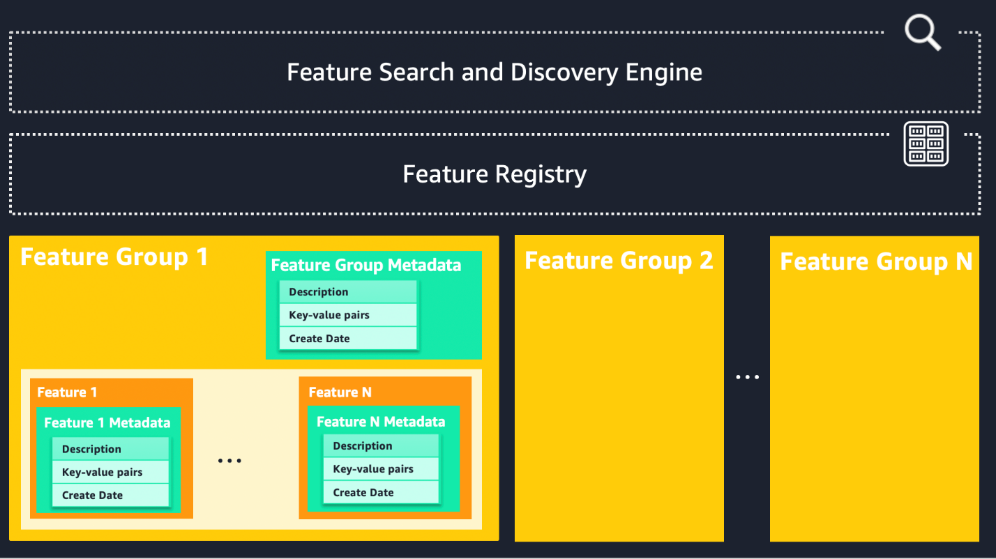
With Feature Store, you have always been able to add metadata at the feature group level. Data scientists who want the ability to search and discover existing features for their models now have the ability to search for information at the feature level by adding custom metadata. For example, the information can include a description of the feature, the date it was last modified, its original data source, certain metrics, or the level of sensitivity.

The following diagram illustrates the architecture relationships between feature groups, features, and associated metadata. Note how data scientists can now specify descriptions and metadata at both the feature group level and the individual feature level.

In this post, we explain how data scientists and ML engineers can use feature-level metadata with the new search and discovery capabilities of Feature Store to promote better feature reuse across their organization. This capability can significantly help data scientists in the feature selection process and, as a result, help you identify features that lead to increased model accuracy.

Use case

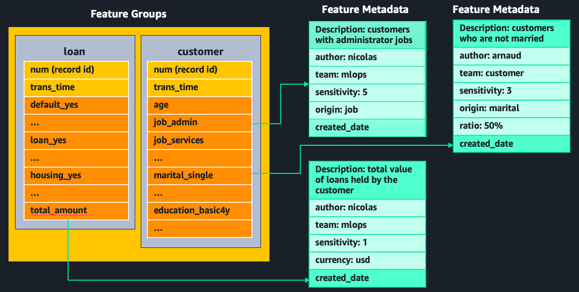
For the purposes of this post, we use two feature groups, customer and loan.

The customer feature group has the following features:

  • age – Customer’s age (numeric)
  • job – Type of job (one-hot encoded, such as admin or services)
  • marital – Marital status (one-hot encoded, such as married or single)
  • education – Level of education (one-hot encoded, such as basic 4y or high school)

The loan feature group has the following features:

  • default – Has credit in default? (one-hot encoded: no or yes)
  • housing – Has housing loan? (one-hot encoded: no or yes)
  • loan – Has personal loan? (one-hot encoded: no or yes)
  • total_amount – Total amount of loans (numeric)

The following figure shows example feature groups and feature metadata.

The purpose of adding a description and assigning metadata to each feature is to increase the speed of discovery by enabling new search parameters along which a data scientist or ML engineer can explore features. These can reflect details about a feature such as its calculation, whether it’s an average over 6 months or 1 year, origin, creator or owner, what the feature means, and more.

In the following sections, we provide two approaches to search and discover features and configure feature-level metadata: the first using Amazon SageMaker Studio directly, and the second programmatically.

Feature discovery in Studio

You can easily search and query features using Studio. With the new enhanced search and discovery capabilities, you can immediately retrieve results using a simple type-ahead of a few characters.

The following screenshot demonstrates the following capabilities:

  • You can access the Feature Catalog tab and observe features across feature groups. The features are presented in a table that includes the feature name, type, description, parameters, date of creation, and associated feature group’s name.
  • You can directly use the type-ahead functionality to immediately return search results.
  • You have the flexibility to use different types of filter options: All, Feature name, Description, or Parameters. Note that All will return all features where either Feature name, Description, or Parameters match the search criteria.
  • You can narrow down the search further by specifying a date range using the Created from and Created to fields and specifying parameters using the Search parameter key and Search parameter value fields.

After you have selected a feature, you can choose the feature’s name to bring up its details. When you choose Edit Metadata, you can add a description and up to 25 key-value parameters, as shown in the following screenshot. Within this view, you can ultimately create, view, update, and delete the feature’s metadata. The following screenshot illustrates how to edit feature metadata for total_amount.

As previously stated, adding key-value pairs to a feature gives you more dimensions along which to search for their given features. For our example, the feature’s origin has been added to every feature’s metadata. When you choose the search icon and filter along the key-value pair origin: job, you can see all the features that were one-hot-encoded from this base attribute.

Feature discovery using code

You can also access and update feature information through the AWS Command Line Interface (AWS CLI) and SDK (Boto3) rather than directly through the AWS Management Console. This allows you to integrate the feature-level search functionality of Feature Store with your own custom data science platforms. In this section, we interact with the Boto3 API endpoints to update and search feature metadata.

To begin improving feature search and discovery, you can add metadata using the update_feature_metadata API. In addition to the description and created_date fields, you can add up to 25 parameters (key-value pairs) to a given feature.

The following code is an example of five possible key-value parameters that have been added to the job_admin feature. This feature was created, along with job_services and job_none, by one-hot-encoding job.

sagemaker_client.update_feature_metadata(
    FeatureGroupName="customer",
    FeatureName="job_admin",
    ParameterAdditions=[
        {"Key": "author", "Value": "arnaud"}, # Feature's author
        {"Key": "team", "Value": "mlops"}, # Team owning the feature
        {"Key": "origin", "Value": "job"}, # Raw input parameter
        {"Key": "sensitivity", "Value": "5"}, # 1-5 scale for data sensitivity
        {"Key": "env", "Value": "testing"} # Environment the feature is used in
    ]
)

After author, team, origin, sensitivity, and env have been added to the job_admin feature, data scientists or ML engineers can retrieve them by calling the describe_feature_metadata API. You can navigate to the Parameters object in the response for the metadata we previously added to our feature. The describe_feature_metadata API endpoint allows you to get greater insight into a given feature by getting its associated metadata.

response = sagemaker_client.describe_feature_metadata(
    FeatureGroupName="customer",
    FeatureName="job_admin",
)

# Navigate to 'Parameters' in response to get metadata
metadata = response['Parameters']

You can search for features by using the SageMaker search API using metadata as search parameters. The following code is an example function that takes a search_string parameter as an input and returns all features where the feature’s name, description, or parameters match the condition:

def search_features_using_string(search_string):
    response = sagemaker_client.search(
        Resource= "FeatureMetadata",
        SearchExpression={
            'Filters': [
               {
                   'Name': 'FeatureName',
                   'Operator': 'Contains',
                   'Value': search_string
               },
               {
                   'Name': 'Description',
                   'Operator': 'Contains',
                   'Value': search_string
               },
               {
                   'Name': 'AllParameters',
                   'Operator': 'Contains',
                   'Value': search_string
               }
           ],
           "Operator": "Or"
        },
    )

    # Displaying results in a pandas DataFrame
    df=pd.json_normalize(response['Results'], max_level=1)
    df.columns = df.columns.map(lambda col: col.split(".")[1])
    df=df.drop('FeatureGroupArn', axis=1)

    return df

The following code snippet uses our search_features function to retrieve all features for which either the feature name, description, or parameters contain the word job:

search_results = search_features_using_string('mlops')
search_results

The following screenshot contains the list of matching feature names as well as their corresponding metadata, including timestamps for each feature’s creation and last modification. You can use this information to improve discovery and visibility into your organization’s features.

Conclusion

SageMaker Feature Store provides a purpose-built feature management solution to help organizations scale ML development across business units and data science teams. Improving feature reuse and feature consistency are primary benefits of a feature store. In this post, we explained how you can use feature-level metadata to improve search and discovery of features. This included creating metadata around a variety of use cases and using it as additional search parameters.

Give it a try, and let us know what you think in comments. If you want to learn more about collaborating and sharing features within Feature Store, refer to Enable feature reuse across accounts and teams using Amazon SageMaker Feature Store.


About the authors

Arnaud Lauer is a Senior Partner Solutions Architect in the Public Sector team at AWS. He enables partners and customers to understand how best to use AWS technologies to translate business needs into solutions. He brings more than 16 years of experience in delivering and architecting digital transformation projects across a range of industries, including the public sector, energy, and consumer goods. Artificial intelligence and machine learning are some of his passions. Arnaud holds 12 AWS certifications, including the ML Specialty Certification.

Nicolas Bernier is an Associate Solutions Architect, part of the Canadian Public Sector team at AWS. He is currently conducting a master’s degree with a research area in Deep Learning and holds five AWS certifications, including the ML Specialty Certification. Nicolas is passionate about helping customers deepen their knowledge of AWS by working with them to translate their business challenges into technical solutions.

Mark Roy is a Principal Machine Learning Architect for AWS, helping customers design and build AI/ML solutions. Mark’s work covers a wide range of ML use cases, with a primary interest in computer vision, deep learning, and scaling ML across the enterprise. He has helped companies in many industries, including insurance, financial services, media and entertainment, healthcare, utilities, and manufacturing. Mark holds six AWS certifications, including the ML Specialty Certification. Prior to joining AWS, Mark was an architect, developer, and technology leader for over 25 years, including 19 years in financial services.

Khushboo Srivastava is a Senior Product Manager for Amazon SageMaker. She enjoys building products that simplify machine learning workflows for customers. In her spare time, she enjoys playing violin, practicing yoga, and traveling.

Read More

Efficient Sequence Modeling for On-Device ML

The increasing demand for machine learning (ML) model inference on-device (for mobile devices, tablets, etc.) is driven by the rise of compute-intensive applications, the need to keep certain data on device for privacy and security reasons, and the desire to provide services when a network connection may not be available. However, on-device inference introduces a myriad of challenges, ranging from modeling to platform support requirements. These challenges relate to how different architectures are designed to optimize memory and computation, while still trying to maintain the quality of the model. From a platform perspective, the issue is identifying operations and building on top of them in a way that can generalize well across different product use cases.

In previous research, we combined a novel technique for generating embeddings (called projection-based embeddings) with efficient architectures like QRNN (pQRNN) and proved them to be competent for a number of classification problems. Augmenting these with distillation techniques provides an additional bump in end-to-end quality. Although this is an effective approach, it is not scalable to bigger and more extensive vocabularies (i.e., all possible Unicode or word tokens that can be fed to the model). Additionally, the output from the projection operation itself doesn’t contain trainable weights to take advantage of pre-training the model.

Token-free models presented in ByT5 are a good starting point for on-device modeling that can address pre-training and scalability issues without the need to increase the size of the model. This is possible because these approaches treat text inputs as a stream of bytes (each byte has a value that ranges from 0 to 255) that can reduce the vocabulary size for the embedding tables from ~30,000 to 256. Although ByT5 presents a compelling alternative for on-device modeling, going from word-level representation to byte stream representation increases the sequence lengths linearly; with an average word length of four characters and a single character having up to four bytes, the byte sequence length increases proportionally to the word length. This can lead to a significant increase in inference latency and computational costs.

We address this problem by developing and releasing three novel byte-stream sequence models for the SeqFlowLite library (ByteQRNN, ByteTransformer and ByteFunnelTransformer), all of which can be pre-trained on unsupervised data and can be fine-tuned for specific tasks. These models leverage recent innovations introduced by Charformer, including a fast character Transformer-based model that uses a gradient-based subword tokenization (GBST) approach to operate directly at the byte level, as well as a “soft” tokenization approach, which allows us to learn token boundaries and reduce sequence lengths. In this post, we focus on ByteQRNN and demonstrate that the performance of a pre-trained ByteQRNN model is comparable to BERT, despite being 300x smaller.

Sequence Model Architecture
We leverage pQRNN, ByT5 and Charformer along with platform optimizations, such as in-training quantization (which tracks minimum and maximum float values for model activations and weights for quantizing the inference model) that reduces model sizes by one-fourth, to develop an end-to-end model called ByteQRNN (shown below). First, we use a ByteSplitter operation to split the input string into a byte stream and feed it to a smaller embedding table that has a vocabulary size of 259 (256 + 3 additional meta tokens).

The output from the embedding layer is fed to the GBST layer, which is equipped with in-training quantization and combines byte-level representations with the efficiency of subword tokenization while enabling end-to-end learning of latent subwords. We “soft” tokenize the byte stream sequences by enumerating and combining each subword block length with scores (computed with a quantized dense layer) at each strided token position (i.e., at token positions that are selected at regular intervals). Next, we downsample the byte stream to manageable sequence length and feed it to the encoder layer.

The output from the GBST layer can be downsampled to a lower sequence length for efficient encoder computation or can be used by an encoder, like Funnel Transformer, which pools the query length and reduces the self-attention computation to create the ByteFunnelTransformer model. The encoder in the end-to-end model can be replaced with any other encoder layer, such as the Transformer from the SeqFlowLite library, to create a ByteTransformer model.

A diagram of a generic end-to-end sequence model using byte stream input. The ByteQRNN model uses a QRNN encoder from the SeqFlowLite library.

In addition to the input embeddings (i.e., the output from the embedding layer described above), we go a step further to build an effective sequence-to-sequence (seq2seq) model. We do so by taking ByteQRNN and adding a Transformer-based decoder model along with a quantized beam search (or tree exploration) to go with it. The quantized beam search module reduces the inference latency when generating decoder outputs by computing the most likely beams (i.e., possible output sequences) using the logarithmic sum of previous and current probabilities and returns the resulting top beams. Here the system uses a more efficient 8-bit integer (uint8) format, compared to a typical single-precision floating-point format (float32) model.

The decoder Transformer model uses a merged attention sublayer (MAtt) to reduce the complexity of the decoder self-attention from quadratic to linear, thereby lowering the end-to-end latency. For each decoding step, MAtt uses a fixed-size cache for decoder self-attention compared to the increasing cache size of a traditional transformer decoder. The following figure illustrates how the beam search module interacts with the decoder layer to generate output tokens on-device using an edge device (e.g., mobile phones, tablets, etc.).

A comparison of cloud server decoding and on-device (edge device) implementation. Left: Cloud server beam search employs a Transformer-based decoder model with quadratic time self-attention in float32, which has an increasing cache size for each decoding step. Right: The edge device implementation employs a quantized beam search module along with a fixed-size cache and a linear time self-attention computation.

Evaluation
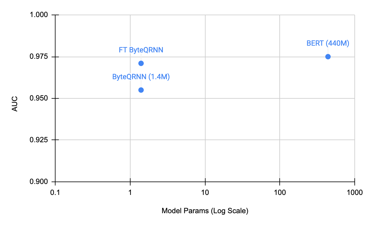
After developing ByteQRNN, we evaluate its performance on the civil_comments dataset using the area under the curve (AUC) metric and compare it to a pre-trained ByteQRNN and BERT (shown below). We demonstrate that the fine-tuned ByteQRNN improves the overall quality and brings its performance closer to the BERT models, despite being 300x smaller. Since SeqFlowLite models support in-training quantization that reduces model sizes by one-fourth, the resulting models scale well to low-compute devices. We chose multilingual data sources that related to the task for pre-training both BERT and byte stream models to achieve the best possible performance.

Comparison of ByteQRNN with fine-tuned ByteQRNN and BERT on the civil_comments dataset.

Conclusion
Following up on our previous work with pQRNN, we evaluate byte stream models for on-device use to enable pre-training and thereby improve model performance for on-device deployment. We present an evaluation for ByteQRNN with and without pre-training and demonstrate that the performance of the pre-trained ByteQRNN is comparable to BERT, despite being 300x smaller. In addition to ByteQRNN, we are also releasing ByteTransformer and ByteFunnelTransformer, two models which use different encoders, along with the merged attention decoder model and the beam search driver to run the inference through the SeqFlowLite library. We hope these models will provide researchers and product developers with valuable resources for future on-device deployments.

Acknowledgements
We would like to thank Khoa Trinh, Jeongwoo Ko, Peter Young and Yicheng Fan for helping with open-sourcing and evaluating the model. Thanks to Prabhu Kaliamoorthi for all the brainstorming and ideation. Thanks to Vinh Tran, Jai Gupta and Yi Tay for their help with pre-training byte stream models. Thanks to Ruoxin Sang, Haoyu Zhang, Ce Zheng, Chuanhao Zhuge and Jieying Luo for helping with the TPU training. Many thanks to Erik Vee, Ravi Kumar and the Learn2Compress leadership for sponsoring the project and their support and encouragement. Finally, we would like to thank Tom Small for the animated figure used in this post.

Read More

NVIDIA Jetson AGX Orin 32GB Production Modules Now Available; Partner Ecosystem Appliances and Servers Arrive

Bringing new AI and robotics applications and products to market, or supporting existing ones, can be challenging for developers and enterprises.

The NVIDIA Jetson AGX Orin 32GB production module — available now — is here to help.

Nearly three dozen technology providers in the NVIDIA Partner Network worldwide are offering commercially available products powered by the new module, which provides up to a 6x performance leap over the previous generation.

With a wide range of offerings from Jetson partners, developers can build and deploy feature-packed Orin-powered systems sporting cameras, sensors, software and connectivity suited for edge AI, robotics, AIoT and embedded applications.

Production-ready systems with options for peripherals enable customers to tackle challenges in industries from manufacturing, retail and construction to agriculture,  logistics, healthcare, smart cities, last-mile delivery and more.

Helping Build More Capable AI-Driven Products Faster 

Traditionally, developers and engineers have been limited in their ability to handle multiple concurrent data streams for complex application environments. They’ve faced strict latency requirements, energy-efficiency constraints, and issues with high-bandwidth wireless connectivity. And they need to be able to easily manage over-the-air software updates.

They’ve also been forced to include multiple chips in their designs to harness the compute resources needed to process diverse, ever-growing amounts of data.

NVIDIA Jetson AGX Orin overcomes all of these challenges.

The Jetson AGX Orin developer kit, capable of up to 275 trillion operations per second, supports multiple concurrent AI application pipelines with an NVIDIA Ampere architecture GPU, next-generation deep learning and vision accelerators, high-speed I/O, and fast memory bandwidth.

With Jetson AGX Orin, customers can develop solutions using the largest and most complex AI models to solve problems such as natural language understanding, 3D perception and multi-sensor fusion.

The four Jetson Orin-based production modules, announced at GTC, offer customers a full range of server-class AI performance. The Jetson AGX Orin 32GB module is available to purchase now, while the 64GB version will be available in November. Two Orin NX production modules are coming later this year.

The production systems are supported by the NVIDIA Jetson software stack, which has enabled thousands of enterprises and millions of developers to build and deploy fully accelerated AI solutions on Jetson.

On top of JetPack SDK, which includes the NVIDIA CUDA-X accelerated stack, Jetson Orin supports multiple NVIDIA platforms and frameworks such as Isaac for robotics, DeepStream for computer vision, Riva for natural language understanding, TAO Toolkit to accelerate model development with pretrained models, and Metropolis, an application framework, set of developer tools and partner ecosystem that brings visual data and AI together to improve operational efficiency and safety across industries.

Customers are bringing their next-generation edge AI and robotics applications to market much faster by first emulating any Jetson Orin-based production module on the Jetson AGX Orin developer kit.

Expanding Developer Community and Jetson Partner Ecosystem 

More than 1 million developers and over 6,000 companies are building commercial products on the NVIDIA Jetson edge AI and robotics computing platform to create and deploy autonomous machines and edge AI applications.

With over 150 members, the growing Jetson ecosystem of partners offers a vast range of support, including from companies specialized in AI software, hardware and application design services, cameras, sensors and peripherals, developer tools and development systems.

Some 32 partners offer commercially available products, powered by the new Jetson AGX Orin module, that are packed with options to help support cutting-edge applications and accelerate time to market.

Developers looking for carrier boards and full hardware systems will find a range of options from AAEON, Auvidea, Connect Tech, MiiVii, Plink-AI, Realtimes and TZTEK to serve their needs.

Over 350 camera and sensor options are available from Allied Vision, Appropho, Basler AG, e-Con Systems, Framos, Leopard Imaging, LIPS, Robosense, Shenzhen Sensing, Stereolabs, Thundersoft, Unicorecomm and Velodyne. These can support challenging indoor/outdoor lighting conditions, as well as capabilities like lidars for mapping, localization and navigation in robotics and autonomous machines.

For comprehensive software support like device management, operating systems (Yocto & Realtime OS), AI software and toolkits, developers can look to Allxon, Cogniteam, Concurrent Realtime, Deci AI, DriveU, Novauto, RidgeRun, and Sequitur Labs.

And for connectivity options, including WiFi 6/6E, LTE and 5G, developers can check out the product offerings from Telit, Quectel, Infineon and Silex.

The new NVIDIA Jetson AGX Orin 32GB production module is available in the Jetson store from retail and distribution partners worldwide.  

The post NVIDIA Jetson AGX Orin 32GB Production Modules Now Available; Partner Ecosystem Appliances and Servers Arrive appeared first on NVIDIA Blog.

Read More

Music to the Gears: NVIDIA’s Clément Farabet on Orchestrating AI Training for Autonomous Vehicles

Autonomous vehicles are one of the most complex AI challenges of our time. For AVs to operate safely in the real world, the networks running within them must come together as an intricate symphony, which requires intensive training, testing and validation on massive amounts of data.

Clément Farabet, vice president of AI infrastructure at NVIDIA, is a proverbial maestro behind the AV development orchestra. He’s applying nearly 15 years of experience in deep learning — including building Twitter’s AI machine — to teach neural networks how to perceive and react to the world around them.

Farabet sat down with NVIDIA’s Katie Burke Washabaugh on the latest episode of the AI Podcast to discuss how the early days of deep learning led to today’s flourishing AV industry, and how he’s approaching deep neural network development.

Tapping into the NVIDIA SaturnV supercomputer, Farabet is designing a highly scalable data factory to deliver intelligent transportation in the near term, while looking ahead to the next frontiers in AI.

You Might Also Like

Lucid Motors’ Mike Bell on Software-Defined Innovation for the Luxury EV Brand

AI and electric-vehicle technology breakthroughs are transforming the automotive industry. These developments pave the way for new innovators, attracting technical prowess and design philosophies from Silicon Valley. Hear how Lucid Motors is applying a tech-industry mindset to develop software-defined vehicles that are always at the cutting edge.

Driver’s Ed: How Waabi Uses AI, Simulation to Teach Autonomous Vehicles to Drive

Teaching the AI brains of autonomous vehicles to understand the world as humans do requires billions of miles of driving experience. The road to achieving this astronomical level of driving leads to the virtual world. Learn how Waabi uses powerful high-fidelity simulations to train and develop production-level autonomous vehicles.

Polestar’s Dennis Nobelius on the Sustainable Performance Brand’s Plans

Driving enjoyment and autonomous driving capabilities can complement one another in intelligent, sustainable vehicles. Learn about the automaker’s plans to unveil its third vehicle, the Polestar 3, the tech inside it, and what the company’s racing heritage brings to the intersection of smarts and sustainability.

Subscribe to the AI Podcast: Now Available on Amazon Music

The AI Podcast is now available through Amazon Music.

In addition, get the AI Podcast through iTunes, Google Podcasts, Google Play, Castbox, DoggCatcher, Overcast, PlayerFM, Pocket Casts, Podbay, PodBean, PodCruncher, PodKicker, Soundcloud, Spotify, Stitcher and TuneIn.

Make the AI Podcast better: Have a few minutes to spare? Fill out this listener survey.

The post Music to the Gears: NVIDIA’s Clément Farabet on Orchestrating AI Training for Autonomous Vehicles appeared first on NVIDIA Blog.

Read More

New algorithm aces university math course questions

Multivariable calculus, differential equations, linear algebra — topics that many MIT students can ace without breaking a sweat — have consistently stumped machine learning models. The best models have only been able to answer elementary or high school-level math questions, and they don’t always find the correct solutions.

Now, a multidisciplinary team of researchers from MIT and elsewhere, led by Iddo Drori, a lecturer in the MIT Department of Electrical Engineering and Computer Science (EECS), has used a neural network model to solve university-level math problems in a few seconds at a human level.

The model also automatically explains solutions and rapidly generates new problems in university math subjects. When the researchers showed these machine-generated questions to university students, the students were unable to tell whether the questions were generated by an algorithm or a human.

This work could be used to streamline content generation for courses, which could be especially useful in large residential courses and massive open online courses (MOOCs) that have thousands of students. The system could also be used as an automated tutor that shows students the steps involved in solving undergraduate math problems.

“We think this will improve higher education,” says Drori, the work’s lead author who is also an adjunct associate professor in the Department of Computer Science at Columbia University, and who will join the faculty at Boston University this summer. “It will help students improve, and it will help teachers create new content, and it could help increase the level of difficulty in some courses. It also allows us to build a graph of questions and courses, which helps us understand the relationship between courses and their pre-requisites, not just by historically contemplating them, but based on data.”

The work is a collaboration including students, researchers, and faculty at MIT, Columbia University, Harvard University, and the University of Waterloo. The senior author is Gilbert Strang, a professor of mathematics at MIT. The research appears this week in the Proceedings of the National Academy of Sciences.

A “eureka” moment

Drori and his students and colleagues have been working on this project for nearly two years. They were finding that models pretrained using text only could not do better than 8 percent accuracy on high school math problems, and those using graph neural networks could ace machine learning course questions but would take a week to train.

Then Drori had what he describes as a “eureka” moment: He decided to try taking questions from undergraduate math courses offered by MIT and one from Columbia University that had never been seen before by a model, turning them into programming tasks, and applying techniques known as program synthesis and few-shot learning. Turning a question into a programming task could be as simple as rewriting the question “find the distance between two points” as “write a program that finds the difference between two points,” or providing a few question-program pairs as examples.

Before feeding those programming tasks to a neural network, however, the researchers added a new step that enabled it to vastly outperform their previous attempts.

In the past, they and others who’ve approached this problem have used a neural network, such as GPT-3, that was pretrained on text only, meaning it was shown millions of examples of text to learn the patterns of natural language. This time, they used a neural network pretrained on text that was also “fine-tuned” on code. This network, called Codex, was produced by OpenAI. Fine-tuning is essentially another pretraining step that can improve the performance of a machine-learning model.

The pretrained model was shown millions of examples of code from online repositories. Because this model’s training data included millions of natural language words as well as millions of lines of code, it learns the relationships between pieces of text and pieces of code.

Many math problems can be solved using a computational graph or tree, but it is difficult to turn a problem written in text into this type of representation, Drori explains. Because this model has learned the relationships between text and code, however, it can turn a text question into code, given just a few question-code examples, and then run the code to answer the problem.

“When you just ask a question in text, it is hard for a machine-learning model to come up with an answer, even though the answer may be in the text,” he says. “This work fills in the that missing piece of using code and program synthesis.”

This work is the first to solve undergraduate math problems and moves the needle from 8 percent accuracy to over 80 percent, Drori adds.

Adding context

Turning math questions into programming tasks is not always simple, Drori says. Some problems require researchers to add context so the neural network can process the question correctly. A student would pick up this context while taking the course, but a neural network doesn’t have this background knowledge unless the researchers specify it.

For instance, they might need to clarify that the “network” in a question’s text refers to “neural networks” rather than “communications networks.” Or they might need to tell the model which programming package to use. They may also need to provide certain definitions; in a question about poker hands, they may need to tell the model that each deck contains 52 cards.

They automatically feed these programming tasks, with the included context and examples, to the pretrained and fine-tuned neural network, which outputs a program that usually produces the correct answer. It was correct for more than 80 percent of the questions.

The researchers also used their model to generate questions by giving the neural network a series of math problems on a topic and then asking it to create a new one.

“In some topics, it surprised us. For example, there were questions about quantum detection of horizontal and vertical lines, and it generated new questions about quantum detection of diagonal lines. So, it is not just generating new questions by replacing values and variables in the existing questions,” Drori says.

Human-generated vs. machine-generated questions

The researchers tested the machine-generated questions by showing them to university students. The researchers gave students 10 questions from each undergraduate math course in a random order; five were created by humans and five were machine-generated.

Students were unable to tell whether the machine-generated questions were produced by an algorithm or a human, and they gave human-generated and machine-generated questions similar marks for level of difficulty and appropriateness for the course.

Drori is quick to point out that this work is not intended to replace human professors.

“Automation is now at 80 percent, but automation will never be 100 percent accurate. Every time you solve something, someone will come up with a harder question. But this work opens the field for people to start solving harder and harder questions with machine learning. We think it will have a great impact on higher education,” he says.

The team is excited by the success of their approach, and have extended the work to handle math proofs, but there are some limitations they plan to tackle. Currently, the model isn’t able to answer questions with a visual component and cannot solve problems that are computationally intractable due to computational complexity.

In addition to overcoming these hurdles, they are working to scale the model up to hundreds of courses. With those hundreds of courses, they will generate more data that can enhance automation and provide insights into course design and curricula.

Read More

Scale YOLOv5 inference with Amazon SageMaker endpoints and AWS Lambda

After data scientists carefully come up with a satisfying machine learning (ML) model, the model must be deployed to be easily accessible for inference by other members of the organization. However, deploying models at scale with optimized cost and compute efficiencies can be a daunting and cumbersome task. Amazon SageMaker endpoints provide an easily scalable and cost-optimized solution for model deployment. The YOLOv5 model, distributed under the GPLv3 license, is a popular object detection model known for its runtime efficiency as well as detection accuracy. In this post, we demonstrate how to host a pre-trained YOLOv5 model on SageMaker endpoints and use AWS Lambda functions to invoke these endpoints.

Solution overview

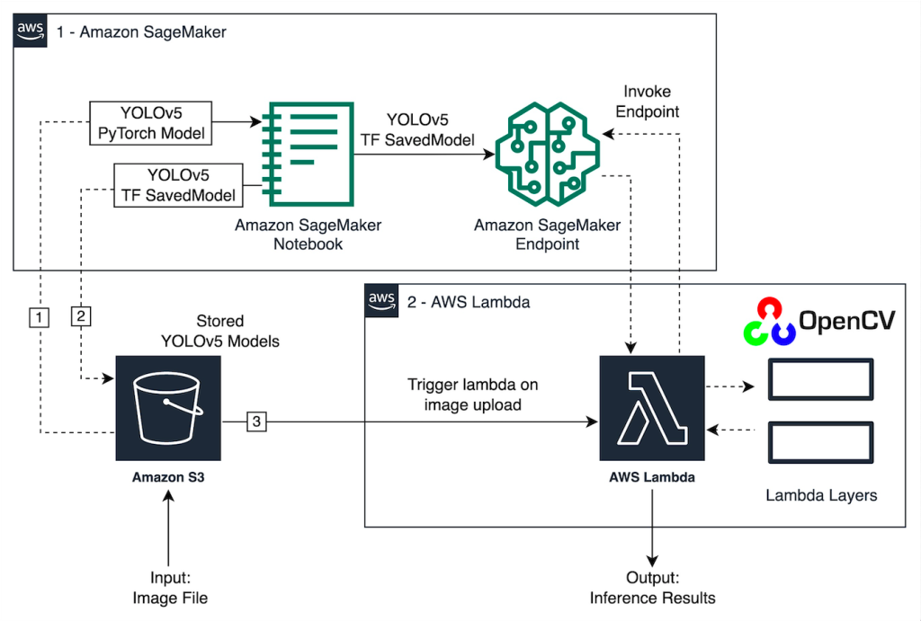
The following image outlines the AWS services used to host the YOLOv5 model using a SageMaker endpoint and invoke the endpoint using Lambda. The SageMaker notebook accesses a YOLOv5 PyTorch model from an Amazon Simple Storage Service (Amazon S3) bucket, converts it to YOLOv5 TensorFlow SavedModel format, and stores it back to the S3 bucket. This model is then used when hosting the endpoint. When an image is uploaded to Amazon S3, it acts as a trigger to run the Lambda function. The function utilizes OpenCV Lambda layers to read the uploaded image and run inference using the endpoint. After the inference is run, you can use the results obtained from it as needed.

AWS architecture

In this post, we walk through the process of utilizing a YOLOv5 default model in PyTorch and converting it to a TensorFlow SavedModel. This model is hosted using a SageMaker endpoint. Then we create and publish a Lambda function that invokes the endpoint to run inference. Pre-trained YOLOv5 models are available on GitHub. For the purpose of this post, we use the yolov5l model.

Prerequisites

As a prerequisite, we need to set up the following AWS Identity and Access Management (IAM) roles with appropriate access policies for SageMaker, Lambda, and Amazon S3:

  • SageMaker IAM role – This requires AmazonS3FullAccess policies attached for storing and accessing the model in the S3 bucket
  • Lambda IAM role – This role needs multiple policies:

    • To access images stored in Amazon S3, we require the following IAM policies:
      • s3:GetObject
      • s3:ListBucket
    • To run the SageMaker endpoint, we need access to the following IAM policies:
      • sagemaker:ListEndpoints
      • sagemaker:DescribeEndpoint
      • sagemaker:InvokeEndpoint
      • sagemaker:InvokeEndpointAsync

You also need the following resources and services:

  • The AWS Command Line Interface (AWS CLI), which we use to create and configure Lambda.
  • A SageMaker notebook instance. These come with Docker pre-installed, and we use this to create the Lambda layers. To set up the notebook instance, complete the following steps:
    • On the SageMaker console, create a notebook instance and provide the notebook name, instance type (for this post, we use ml.c5.large), IAM role, and other parameters.
    • Clone the public repository and add the YOLOv5 repository provided by Ultralytics.

Host YOLOv5 on a SageMaker endpoint

Before we can host the pre-trained YOLOv5 model on SageMaker, we must export and package it in the correct directory structure inside model.tar.gz. For this post, we demonstrate how to host YOLOv5 in the saved_model format. The YOLOv5 repo provides an export.py file that can export the model in many different ways. After you clone the YOLOv5 and enter the YOLOv5 directory from command line, you can export the model with the following command:

$ cd yolov5
$ pip install -r requirements.txt tensorflow-cpu
$ python export.py --weights yolov5l.pt --include saved_model --nms

This command creates a new directory called yolov5l_saved_model inside the yolov5 directory. Inside the yolov5l_saved_model directory, we should see the following items:

yolov5l_saved_model
    ├─ assets
    ├─ variables
    │    ├── variables.data-00000-of-00001
    │    └── variables.index
    └── saved_model.pb

To create a model.tar.gz file, move the contents of yolov5l_saved_model to export/Servo/1. From the command line, we can compress the export directory by running the following command and upload the model to the S3 bucket:

$ mkdir export && mkdir export/Servo
$ mv yolov5l_saved_model export/Servo/1
$ tar -czvf model.tar.gz export/
$ aws s3 cp model.tar.gz "<s3://BUCKET/PATH/model.tar.gz>"

Then, we can deploy a SageMaker endpoint from a SageMaker notebook by running the following code:

import os
import tensorflow as tf
from tensorflow.keras import backend
from sagemaker.tensorflow import TensorFlowModel

model_data = '<s3://BUCKET/PATH/model.tar.gz>'
role = '<IAM ROLE>'

model = TensorFlowModel(model_data=model_data,
                        framework_version='2.8', role=role)

INSTANCE_TYPE = 'ml.m5.xlarge'
ENDPOINT_NAME = 'yolov5l-demo'

predictor = model.deploy(initial_instance_count=1,
                            instance_type=INSTANCE_TYPE,
                            endpoint_name=ENDPOINT_NAME)

The preceding script takes approximately 2–3 minutes to fully deploy the model to the SageMaker endpoint. You can monitor the status of the deployment on the SageMaker console. After the model is hosted successfully, the model is ready for inference.

Test the SageMaker endpoint

After the model is successfully hosted on a SageMaker endpoint, we can test it out, which we do using a blank image. The testing code is as follows:

import numpy as np

ENDPOINT_NAME = 'yolov5l-demo'

modelHeight, modelWidth = 640, 640
blank_image = np.zeros((modelHeight,modelWidth,3), np.uint8)
data = np.array(resized_image.astype(np.float32)/255.)
payload = json.dumps([data.tolist()])
response = runtime.invoke_endpoint(EndpointName=ENDPOINT_NAME,
ContentType='application/json',
Body=payload)

result = json.loads(response['Body'].read().decode())
print('Results: ', result)

Set up Lambda with layers and triggers

We use OpenCV to demonstrate the model by passing an image and getting the inference results. Lambda doesn’t come with external libraries like OpenCV pre-built, therefore we need to build it before we can invoke the Lambda code. Furthermore, we want to make sure that we don’t build external libraries like OpenCV every time Lambda is being invoked. For this purpose, Lambda provides a functionality to create Lambda layers. We can define what goes in these layers, and they can be consumed by the Lambda code every time it’s invoked. We also demonstrate how to create the Lambda layers for OpenCV. For this post, we use an Amazon Elastic Compute Cloud (Amazon EC2) instance to create the layers.

After we have the layers in place, we create the app.py script, which is the Lambda code that uses the layers, runs the inference, and gets results. The following diagram illustrates this workflow.

Lambda permission

Create Lambda layers for OpenCV using Docker

Use Dockerfile as follows to create the Docker image using Python 3.7:

FROM amazonlinux

RUN yum update -y
RUN yum install gcc openssl-devel bzip2-devel libffi-devel wget tar gzip zip make -y

# Install Python 3.7
WORKDIR /
RUN wget https://www.python.org/ftp/python/3.7.12/Python-3.7.12.tgz
RUN tar -xzvf Python-3.7.12.tgz
WORKDIR /Python-3.7.12
RUN ./configure --enable-optimizations
RUN make altinstall

# Install Python packages
RUN mkdir /packages
RUN echo "opencv-python" >> /packages/requirements.txt
RUN mkdir -p /packages/opencv-python-3.7/python/lib/python3.7/site-packages
RUN pip3.7 install -r /packages/requirements.txt -t /packages/opencv-python-3.7/python/lib/python3.7/site-packages

# Create zip files for Lambda Layer deployment
WORKDIR /packages/opencv-python-3.7/
RUN zip -r9 /packages/cv2-python37.zip .
WORKDIR /packages/
RUN rm -rf /packages/opencv-python-3.7/

Build and run Docker and store the output ZIP file in the current directory under layers:

$ docker build --tag aws-lambda-layers:latest <PATH/TO/Dockerfile>
$ docker run -rm -it -v $(pwd):/layers aws-lambda-layers cp /packages/cv2-python37.zip /layers

Now we can upload the OpenCV layer artifacts to Amazon S3 and create the Lambda layer:

$ aws s3 cp layers/cv2-python37.zip s3://<BUCKET>/<PATH/TO/STORE/ARTIFACTS>
$ aws lambda publish-layer-version --layer-name cv2 --description "Open CV" --content S3Bucket=<BUCKET>,S3Key=<PATH/TO/STORE/ARTIFACTS>/cv2-python37.zip --compatible-runtimes python3.7

After the preceding commands run successfully, you have an OpenCV layer in Lambda, which you can review on the Lambda console.

Lambda console

Create the Lambda function

We utilize the app.py script to create the Lambda function and use OpenCV. In the following code, change the values for BUCKET_NAME and IMAGE_LOCATION to the location for accessing the image:

import os, logging, json, time, urllib.parse
import boto3, botocore
import numpy as np, cv2

logger = logging.getLogger()
logger.setLevel(logging.INFO)
client = boto3.client('lambda')

# S3 BUCKETS DETAILS
s3 = boto3.resource('s3')
BUCKET_NAME = "<NAME OF S3 BUCKET FOR INPUT IMAGE>"
IMAGE_LOCATION = "<S3 PATH TO IMAGE>/image.png"

# INFERENCE ENDPOINT DETAILS
ENDPOINT_NAME = 'yolov5l-demo'
config = botocore.config.Config(read_timeout=80)
runtime = boto3.client('runtime.sagemaker', config=config)
modelHeight, modelWidth = 640, 640

# RUNNING LAMBDA
def lambda_handler(event, context):
    key = urllib.parse.unquote_plus(event['Records'][0]['s3']['object']['key'], encoding='utf-8')

    # INPUTS - Download Image file from S3 to Lambda /tmp/
    input_imagename = key.split('/')[-1]
    logger.info(f'Input Imagename: {input_imagename}')
    s3.Bucket(BUCKET_NAME).download_file(IMAGE_LOCATION + '/' + input_imagename, '/tmp/' + input_imagename)

    # INFERENCE - Invoke the SageMaker Inference Endpoint
    logger.info(f'Starting Inference ... ')
    orig_image = cv2.imread('/tmp/' + input_imagename)
    if orig_image is not None:
        start_time_iter = time.time()
        # pre-processing input image
        image = cv2.resize(orig_image.copy(), (modelWidth, modelHeight), interpolation = cv2.INTER_AREA)
        data = np.array(image.astype(np.float32)/255.)
        payload = json.dumps([data.tolist()])
        # run inference
        response = runtime.invoke_endpoint(EndpointName=ENDPOINT_NAME, ContentType='application/json', Body=payload)
        # get the output results
        result = json.loads(response['Body'].read().decode())
        end_time_iter = time.time()
        # get the total time taken for inference
        inference_time = round((end_time_iter - start_time_iter)*100)/100
    logger.info(f'Inference Completed ... ')

    # OUTPUTS - Using the output to utilize in other services downstream
    return {
        "statusCode": 200,
        "body": json.dumps({
                "message": "Inference Time:// " + str(inference_time) + " seconds.",
                "results": result
                }),
            }

Deploy the Lambda function with the following code:

$ zip app.zip app.py
$ aws s3 cp app.zip s3://<BUCKET>/<PATH/TO/STORE/FUNCTION>
$ aws lambda create-function --function-name yolov5-lambda --handler app.lambda_handler --region us-east-1 --runtime python3.7 --environment "Variables={BUCKET_NAME=$BUCKET_NAME,S3_KEY=$S3_KEY}" --code S3Bucket=<BUCKET>,S3Key="<PATH/TO/STORE/FUNCTION/app.zip>"

Attach the OpenCV layer to the Lambda function

After we have the Lambda function and layer in place, we can connect the layer to the function as follows:

$ aws lambda update-function-configuration --function-name yolov5-lambda --layers cv2

We can review the layer settings via the Lambda console.

Lambda settings

Trigger Lambda when an image is uploaded to Amazon S3

We use an image upload to Amazon S3 as a trigger to run the Lambda function. For instructions, refer to Tutorial: Using an Amazon S3 trigger to invoke a Lambda function.

You should see the following function details on the Lambda console.

function overview

Run inference

After you set up Lambda and the SageMaker endpoint, you can test the output by invoking the Lambda function. We use an image upload to Amazon S3 as a trigger to invoke Lambda, which in turn invokes the endpoint for inference. As an example, we upload the following image to the Amazon S3 location <S3 PATH TO IMAGE>/test_image.png configured in the previous section.

test image

After the image is uploaded, the Lambda function is triggered to download and read the image data and send it to the SageMaker endpoint for inference. The output result from the SageMaker endpoint is obtained and returned by the function in JSON format, which we can use in different ways. The following image shows example output overlayed on the image.

inference result

Clean up

Depending on the instance type, SageMaker notebooks can require significant compute usage and cost. To avoid unnecessary costs, we advise stopping the notebook instance when it’s not in use. Additionally, Lambda functions and SageMaker endpoints incur charges only when they’re invoked. Therefore, no cleanup is necessary for those services. However, if an endpoint isn’t being used any longer, it’s good practice to remove the endpoint and the model.

Conclusion

In this post, we demonstrated how to host a pre-trained YOLOv5 model on a SageMaker endpoint and use Lambda to invoke inference and process the output. The detailed code is available on GitHub.

To learn more about SageMaker endpoints, check out Create your endpoint and deploy your model and Build, test, and deploy your Amazon SageMaker inference models to AWS Lambda, which highlights how you can automate the process of deploying YOLOv5 models.


About the authors

Kevin Song is an IoT Edge Data Scientist at AWS Professional Services. Kevin holds a PhD in Biophysics from The University of Chicago. He has over 4 years of industry experience in Computer Vision and Machine Learning. He is involved in helping customers in the sports and life sciences industry deploy  Machine Learning models.

Romil Shah is an IoT Edge Data Scientist at AWS Professional Services. Romil has over 6 years of industry experience in Computer Vision, Machine Learning and IoT edge devices. He is involved in helping customers optimize and deploy their Machine Learning models for edge devices for industrial setup.

Read More

NeuMan: Neural Human Radiance Field from a Single Video

Photorealistic rendering and reposing of humans is important for enabling augmented reality experiences. We propose a novel framework to reconstruct the human and the scene that can be rendered with novel human poses and views from just a single in-the-wild video. Given a video captured by a moving camera, we train two NeRF models: a human NeRF model and a scene NeRF model. To train these models, we rely on existing methods to estimate the rough geometry of the human and the scene. Those rough geometry estimates allow us to create a warping field from the observation space to the canonical…Apple Machine Learning Research

Why it’s a problem that pulse oximeters don’t work as well on patients of color

Pulse oximetry is a noninvasive test that measures the oxygen saturation level in a patient’s blood, and it has become an important tool for monitoring many patients, including those with Covid-19. But new research links faulty readings from pulse oximeters with racial disparities in health outcomes, potentially leading to higher rates of death and complications such as organ dysfunction, in patients with darker skin.

It is well known that non-white intensive care unit (ICU) patients receive less-accurate readings of their oxygen levels using pulse oximeters — the common devices clamped on patients’ fingers. Now, a paper co-authored by MIT scientists reveals that inaccurate pulse oximeter readings can lead to critically ill patients of color receiving less supplemental oxygen during ICU stays.

The paper,Assessment of Racial and Ethnic Differences in Oxygen Supplementation Among Patients in the Intensive Care Unit,” published in JAMA Internal Medicine, focused on the question of whether there were differences in supplemental oxygen administration among patients of different races and ethnicities that were associated with pulse oximeter performance discrepancies. 

The findings showed that inaccurate readings of Asian, Black, and Hispanic patients resulted in them receiving less supplemental oxygen than white patients. These results provide insight into how health technologies such as the pulse oximeter contribute to racial and ethnic disparities in care, according to the researchers.

The study’s senior author, Leo Anthony Celi, clinical research director and principal research scientist at the MIT Laboratory for Computational Physiology, and a principal research scientist at the MIT Institute for Medical Engineering and Science (IMES), says the challenge is that health care technology is routinely designed around the majority population.

“Medical devices are typically developed in rich countries with white, fit individuals as test subjects,” he explains. “Drugs are evaluated through clinical trials that disproportionately enroll white individuals. Genomics data overwhelmingly come from individuals of European descent.”

“It is therefore not surprising that we observe disparities in outcomes across demographics, with poorer outcomes among those who were not included in the design of health care,” Celi adds.

While pulse oximeters are widely used due to ease of use, the most accurate way to measure blood oxygen saturation (SaO2) levels is by taking a sample of the patient’s arterial blood. False readings of normal pulse oximetry (SpO2) can lead to hidden hypoxemia. Elevated bilirubin in the bloodstream and the use of certain medications in the ICU called vasopressors can also throw off pulse oximetry readings.

More than 3,000 participants were included in the study, of whom 2,667 were white, 207 Black, 112 Hispanic, and 83 Asian — using data from the Medical Information Mart for Intensive Care version 4, or MIMIC-IV dataset. This dataset is comprised of more than 50,000 patients admitted to the ICU at Beth Israel Deaconess Medical Center, and includes both pulse oximeter readings and oxygen saturation levels detected in blood samples. MIMIC-IV also includes rates of administration of supplemental oxygen.

When the researchers compared SpO2 levels taken by pulse oximeter to oxygen saturation from blood samples, they found that Black, Hispanic, and Asian patients had higher SpO2 readings than white patients for a given blood oxygen saturation level measured in blood samples. The turnaround time of arterial blood gas analysis may take from several minutes up to an hour. As a result, clinicians typically make decisions based on pulse oximetry reading, unaware of its suboptimal performance in certain patient demographics.

Eric Gottlieb, the study’s lead author, a nephrologist, a lecturer at MIT, and a Harvard Medical School fellow at Brigham and Women’s Hospital, called for more research to be done, in order to better understand “how pulse oximeter performance disparities lead to worse outcomes; possible differences in ventilation management, fluid resuscitation, triaging decisions, and other aspects of care should be explored. We then need to redesign these devices and properly evaluate them to ensure that they perform equally well for all patients.”

Celi emphasizes that understanding biases that exist within real-world data is crucial in order to better develop algorithms and artificial intelligence to assist clinicians with decision-making. “Before we invest more money on developing artificial intelligence for health care using electronic health records, we have to identify all the drivers of outcome disparities, including those that arise from the use of suboptimally designed technology,” he argues. “Otherwise, we risk perpetuating and magnifying health inequities with AI.”

Celi described the project and research as a testament to the value of data sharing that is the core of the MIMIC project. “No one team has the expertise and perspective to understand all the biases that exist in real-world data to prevent AI from perpetuating health inequities,” he says. “The database we analyzed for this project has more than 30,000 credentialed users consisting of teams that include data scientists, clinicians, and social scientists.”

The many researchers working on this topic together form a community that shares and performs quality checks on codes and queries, promotes reproducibility of the results, and crowdsources the curation of the data, Celi says. “There is harm when health data is not shared,” he says. “Limiting data access means limiting the perspectives with which data is analyzed and interpreted. We’ve seen numerous examples of model mis-specifications and flawed assumptions leading to models that ultimately harm patients.”

Read More