![]()

Real-world decision-making often requires reasoning about when an event will occur. The overarching goal of such reasoning is to help aid decision-making for optimal triage and subsequent intervention. Such problems involving estimation of Times-to-an-Event frequently arise across multiple application areas, including,
Healthcare and Bio-informatics: More commonly known as ‘Survival Analysis‘ involves prognostication of an adverse physiological event like a stroke, the onset of cancer, re-hospitalization, and mortality. Time-to-event or survival analysis can be used to proactively mitigate adverse outcomes and extend the longevity of patients.
Internet Marketing and e-commerce: Models employed for estimating customer churn and retention in large commercial organizations are essentially time-to-event regression models and help determine best practices to maximize customer retention.
Predictive Maintenance: Reliability engineering and systems safety research involves the use of remaining useful life prediction models to help extend the longevity of machinery and equipment by proactive part and component replacement.
Finance and Actuarial and Sciences: Time-to-Event models are ubiquitous in the estimation of optimal financial strategies for setting insurance premiums, as well as estimating credit defaulting behavior.
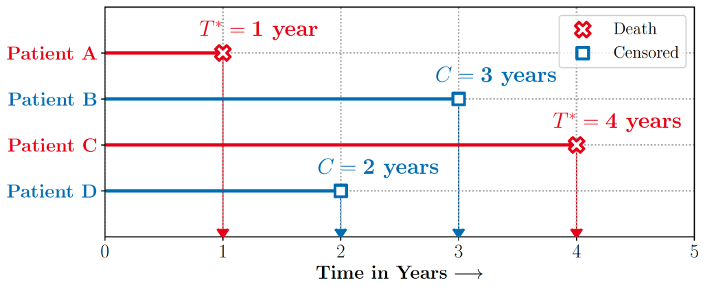
Figure 1 illustrates a typical example of a Time-to-Event problem in healthcare. The challenge of working with time-to-event data is compounded by the fact that as evidenced in the figure, such data typically includes individuals whose outcomes are unobserved, or ‘censored,’ either due to a loss of follow-up or end of the study.
Discretizing time-to-event outcomes to predict if an event will occur is a common approach in standard machine learning. However, this neglects temporal context, which could result in models that misestimate and lead to poorer generalization.
The auton-survival Package
In our recent Machine Learning for Healthcare ’22 paper, we present auton-survival – a comprehensive Python code repository of user-friendly, machine learning tools for working with censored time-to-event data. This package includes an exclusive suite of workflows for a range of tasks from data pre-processing and regression modeling to model evaluation. auton-survival includes an API similar to the scikit-learn package (Pedregosa et al., 2011), making its adoption easy for users with machine learning experience in Python. Additionally, to promote the usability of the package and rapid prototyping of solutions for both machine learning and clinical researchers, we include detailed documentation as well as example notebooks.
Time-to-Event Regression
Time-to-Event or Survival regression can be used to estimate the conditional probability of an event occurring within a specified time period or event-horizon. A time-to-event estimation problem thus reduces to estimating the conditional distribution of survival:
( mathbb{E}[1{T > t}|X = x] = mathbb{P}(T > t|X = x) = 1 − mathbb{P}(T ≤ t|X = x) )
Note that ( X) is a set of covariates, and ( T ) refers to the distribution of the censored survival time ( T = text{min}(T^∗, C) ) where ( T^∗ ) is the distribution of the true time-to-event and ( C ) is the distribution of the censoring time. Assuming conditional independence between ( T ) and ( C ) (ie., ( T ⊥ C|X )) allows identification of the distribution of ( mathbb{P}(T |X) ).
Survival regression naturally allows accounting for censored data. In the case of survival regression, the likelihood ( ell ) under censoring is given as
( ell ({x, t, δ}) ∝ mathbb{P}(T = t|X = x)^δmathbb{P}(T > t|X = x)^{1−δ} ).
Here ( x in mathbb{R}^d ) are the covariates, ( t in mathbb{R}^{+} ) is the event or censoring time and ( delta in {0, 1} ) is a binary indicator denoting if the individual was censored. For the censored individuals, the likelihood corresponds to the probability that the event takes place beyond the time horizon, ( t, mathbb{P}(T > t|X = x) ) also known as the ‘survival function‘.
Broadly, the popular approaches for learning estimators of survival in the presence of censoring can be categorized into:
- Parametric: Assume that time-to-event distribution ( mathbb{P}(T) ) adheres to a known parametric distribution, such as Weibull or Log-Normal.
- Non-Parametric: Involve learning kernels or similarity functions of the input covariates followed by a non-parametric (Kaplan-Meier or Nelson-Aalen) estimation of the survival rate weighted with the learned kernel.
- Semi-Parametric: As with Cox Proportional Hazards models, feature interactions are learned through a parametric model followed by a non-parametric estimation of the base survival (hazard) rate.
Estimators of Survival [Notebook] [Docs]
auton-survival includes flexible estimators of time-to-events in the presence of non-proportional hazards.Complex multimodal data often observed in healthcare and other applications, bring a multitude of challenges to traditional machine learning. auton-survival allows a simple interface to use deep neural networks and representation learning to model such complex data.
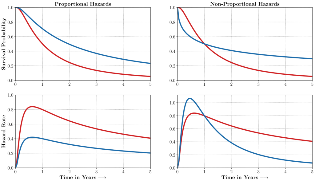
auton-survival includes extensions to the standard Cox Proportional Hazards (CPH) (Cox, 1972) involving deep representation learning (Faraggi and Simon, 1995; Katzman et al., 2018) as well as latent variable survival regression models, Deep Cox Mixtures (DCM), and Deep Survival Machines (DSM) (Nagpal et al., 2021 a,b) that ease the strong assumptions of proportional hazards shown in Figure 2 by modeling the time-to-event distribution as a fixed size mixture.
The SurvivalModel Class
The package provides a convenient SurvivalModel class that enables rapid experimentation via a consistent API that wraps multiple alternative regression estimators. In addition to the models mentioned above, the SurvivalModel class includes Random Survival Forests (RSF) (Ishwaran et al., 2008), which is a popular non-parametric survival model.
Hyperparameter tuning for model selection can be streamlined with the SurvivalRegressionCV class to apply ( K-text{fold} ) cross-validation over a user-specified hyperparameter grid.
Time-Varying Survival Regression
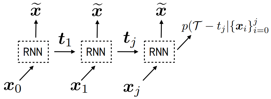
Real-world data often consists of multiple time-dependent observations per individual or time-varying covariates. auton-survival is equipped to handle time-varying covariates for survival analysis with auto-regressive deep learning models that allow learning temporal dependencies when estimating time-to-event outcomes. Implementations of time-varying DSM and Deep Cox Proportional Hazards model involve the use of RNNs, LSTMs, or GRUs (Chung et al., 2014; Hochreiter and Schmidhuber, 1997) for time-varying survival regression as shown in Figure 3.
Counterfactual Estimators of Survival
Decision support often requires reasoning about ‘what if’ scenarios regarding the effect of different treatments on outcomes. In observational settings, outcomes and treatment assignments may share common causes. Adjusting for such confounding factors is crucial when performing causal inference. auton-survival includes counterfactual survival regression as a tool for causal inference that accounts for confounding factors when estimating the effect of treatment on survival. Counterfactual survival regression involves fitting separate regression models on the treated and control populations and computing survival rates across treatment arms. Under the standard causal inference assumption of strong ignorability, the time-to-event outcome under intervention ( text{do}(A = a) ) can then be estimated as
(hat{S}big(t|text{do}(A = a)big) = mathop{mathbb{E}}_{X} big[hat{mathbb{E}}[1{T > t}|X = x, A = a] big] )
where (hat{mathbb{E}}[1{T > t}|X = x, A = a]) is just an estimate of the conditional expectation of survival learnt on the population under intervention ( (A=a) ).
Consider the data from the large SEER Cancer Incidence registry (Ries et al., 1975). When stratified by region (Figure 4a), there is an apparent disparity in survival rates. We demonstrate the use of counterfactual regression to provide insight into whether these discrepancies can be attributed to the geographic region or other socio-economic or physiological confounding factors that affect both belonging to these regions and the outcomes. To adjust estimates of survival with counterfactual estimation, we train two separate Deep Cox models on data from Greater California and Louisiana as counterfactual regressors. The fitted regressors are then applied to estimate the survival curves for each instance, which are then averaged over treatment groups to compute the domain-specific survival rate. Figure 4b presents the counterfactual survival rates compared with the survival rates obtained from a Kaplan-Meier estimator. The Kaplan-Meier estimator does not adjust for confounding factors and overestimates treatment effect, as evidenced by the extent that survival rates differ between regions. Alternatively, counterfactual regression adjusts for confounding factors and predicts more similar survival rates between regions.
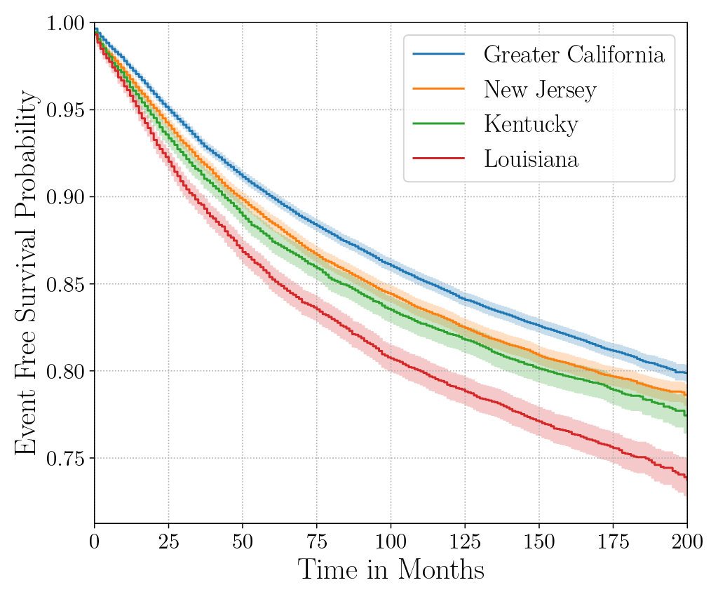
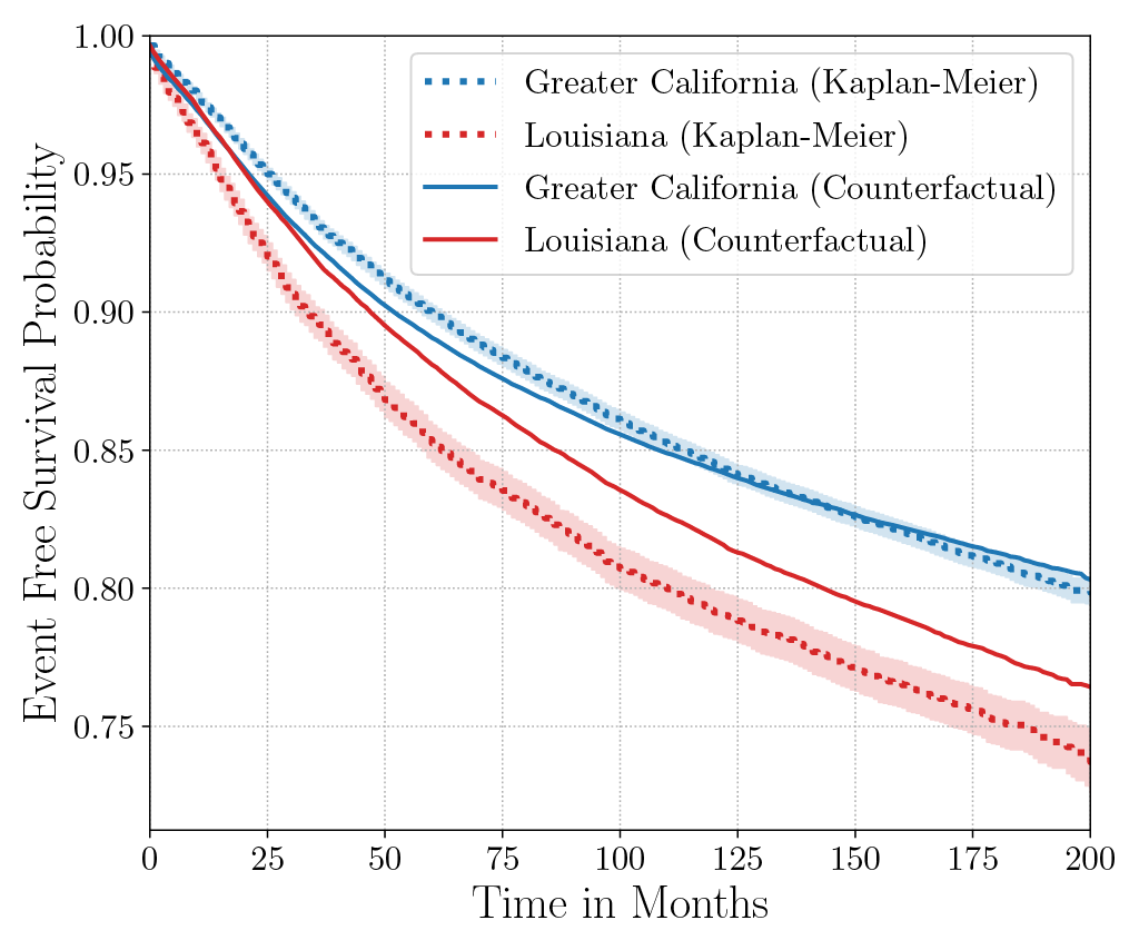
discrepancies in the Kaplan-Meier estimated survival rates when stratified by the geographic
region (left). The Kaplan-Meier estimator overestimates the effect of region on mortality compared with the counterfactual regression model, which reduces discrepancy in survival rates between regions (right).
Phenotyping Censored Survival Data [Notebook] [Docs]
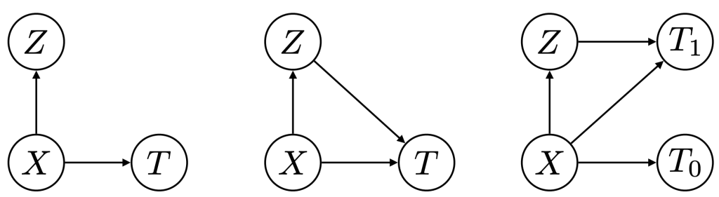
Figure 5: Phenotypers in auton-survival: ( X ) represents the covariates, ( T ) the time-to-event, and ( Z ) is the phenotype to be inferred.
Survival rates differ across groups of individuals with heterogeneous characteristics. Identifying groups of patients with similar survival rates can be used to derive insight into practices and interventions that can help improve longevity for such groups. While domain knowledge can help identify such subgroups, in practice there could be potentially complex, non-linear feature interactions that determine assignment to subgroups, making identification difficult. In auton-survival, we refer to this group identification and survival assessment as phenotyping.
Our package offers multiple approaches to phenotyping that involve either the use of specific domain knowledge, as in the case of the intersectional phenotyper, or a completely unsupervised approach that clusters subjects based on the observed covariates. Additionally, auton-survival also offers phenotypers that explicitly involve supervision in the form of the observed outcomes and counterfactuals inform the learned phenotypes to better stratify the data. Directed Acyclic Graphical representations of probabilistic phenotypers in auton-survival are shown in Figure 5.
- Intersectional Phenotyping: Recovers groups, or phenotypes, of individuals over exhaustive combinations of user-specified categorical and numerical features.
- Unsupervised Phenotyping: Identifies groups of individuals based on structured similarity in the feature space by first performing dimensionality reduction of the input covariates, followed by clustering. The estimated probability of an individual belonging to a latent group is computed as the distance to the cluster normalized by the sum of distances to other clusters.
- Supervised Phenotyping: Identifies latent groups of individuals with similar survival outcomes conditioned on outcomes. This approach can be performed as a direct consequence of training the DSM and DCM latent variable survival estimators.
- Counterfactual Phenotyping: Identifies groups of individuals that demonstrate enhanced or diminished treatment effects (Chirag et al., 2022).
Figure 6 presents the Kaplan-Meier survival curves of the phenogroups extracted from SUPPORT (Knaus et al., 1995) using the unsupervised and supervised phenotyping. The intersecting survival curves suggest the phenotypers’ ability to recover phenogroups that do not strictly adhere to assumptions of Proportional Hazards. From Figure 7, it can be inferred that supervised phenotyping extracts phenogroups with higher discriminative power as indicated by the contrasting Kaplan-Meier estimates of phenogroup level survival.


Figure 6: Kaplan-Meier survival curves of the phenogroups extracted from SUPPORT using the unsupervised and supervised phenotyping.
Treatment Effect Estimation
auton-survival offers additional tools to analyze the effect of an intervention on outcomes by computing propensity-adjusted treatment effects in terms of the following metrics through bootstrap resampling of the dataset with replacement:
- Hazard Ratio: Assuming the proportional hazards assumptions holds, the treatment effect can be measured as the ratio of hazard rates between the treatment and control arms.
- Time at Risk (TaR) (Figure 7a): The treatment effect can be measured as the difference in time-to-event at a specified level of risk.
- Risk at Time (Figure 7b): The treatment effect can be measured as the difference in risk at a specified time horizon.
- Restricted Mean Survival Time (RMST) (Figure 7c): The treatment effect can be measured as the difference in the expected (or mean) time-to-event conditioned on a specified time horizon.
Propensity-adjustment allows an alternative approach to estimate treatment effects of potential confounders that influence both treatment assignment and the outcome. Not adjusting for treatment propensity could result in misestimations of treatment effects.


Figure 7: Treatment effects measured in terms of the difference in metrics computed for
treatment and control groups including (a) the time at a specified level of risk (b) risk at a
certain time and (c) the expected survival time over a truncated time horizon.
auton-survival allows adjusting for treatment propensity with computation of treatment effects bootstrapped with sample weights. When the specified sample weights are propensity scores, such as obtained from a classification model, the bootstrapped distribution treatment effect converges to the Inverse Propensity of Treatment Weighting (IPTW) Thompson-Horvitz estimate of the population Average Treatment Effect.
(mathbb{ATE}(mathcal{D}^*, f) = mathbb{E}_{x sim mathcal{D}^*} big[mathbb{E} [f_1(x) – f_0(x) | X = x]big] ; quad mathcal{D}^* sim frac{1}{widehat{mathbb{P}}(A|X)} cdot mathbb{P}^*(mathcal{D}) )
In a second analysis of the effect of geographical region on breast cancer mortality using data from the SEER cancer registry (Ries et al., 1975), we compare treatment effects before and after adjusting for confounding factors by inverse propensity weighting. Similar to the previous analysis with counterfactual regression, we consider the regions of “Greater California” and “Louisiana” as the binary “treatment” in question. To adjust treatment effects for confounding factors, we first trained a logistic regression with an ( ell_2 ) penalty by regressing the geographical region on the set of confounding variables. The estimated propensity scores are then employed as sampling weights for the treatment effects in terms of hazard ratios, restricted mean survival time (RMST), and risk difference as in Figure 8. Adjusting for region propensity noticeably mitigates differences in treatment effects, indicating that mortality due to breast cancer is likely explained by confounding socio-economic and physiological factors rather than solely the geographic region.


Figure 8: Estimated probability densities of the bootstrapped treatment effects treatment effects before (blue) and after (red) adjusting for treatment propensity by inverse propensity weighting.
Conclusion
We present auton-survival, an open-source Python package encapsulating multiple pipelines to work with censored time-to-event data. Such data is ubiquitous in many fields, including healthcare and the maintenance of equipment. Through continuous collaboration with the machine learning for healthcare community, we aim to better aid machine learning research in efforts to create a robust, comprehensive repository of rigorous tools for reproducible analysis of censored time-to-event data.
Authors
Chirag Nagpal
PhD Candidate, Auton Lab
@nagpalchirag
cs.cmu.edu/~chiragn
Willa Potosnak
Research Intern and
Incoming PhD Student, Auton Lab
potosnakw.github.io
References
[1] Nagpal, C., Potosnak, W. and Dubrawski, A., 2022. auton-survival: an Open-Source Package for Regression, Counterfactual Estimation, Evaluation and Phenotyping with Censored Time-to-Event Data. arXiv preprint arXiv:2204.07276.
[2] Fabian Pedregosa, Ga¨el Varoquaux, Alexandre Gramfort, Vincent Michel, Bertrand Thirion, Olivier Grisel, Mathieu Blondel, Peter Prettenhofer, Ron Weiss, Vincent Dubourg, et al. Scikit-learn: Machine learning in python. the Journal of machine Learning research, 12: 2825–2830, 2011.
[3] D. R. Cox. Regression models and life-tables. Journal of the Royal Statistical Society. Series B (Methodological), 34(2):187–220, 1972.
[4] David Faraggi and Richard Simon. A neural network model for survival data. Statistics in medicine, 14(1):73–82, 1995.
[5] Jared L Katzman, Uri Shaham, Alexander Cloninger, Jonathan Bates, Tingting Jiang, and Yuval Kluger. Deepsurv: personalized treatment recommender system using a cox proportional hazards deep neural network. BMC medical research methodology, 18(1): 1–12, 2018.
[6] Nagpal, C., Li, X. and Dubrawski, A., 2021a. Deep survival machines: Fully parametric survival regression and representation learning for censored data with competing risks. IEEE Journal of Biomedical and Health Informatics, 25(8), pp.3163-3175.
[7] Nagpal, C., Yadlowsky, S., Rostamzadeh, N. and Heller, K., 2021b, October. Deep Cox mixtures for survival regression. In Machine Learning for Healthcare Conference (pp. 674-708). PMLR.
[8] H. Ishwaran, Udaya B. Kogalur, Eugene H. Blackstone, and Michael S. Lauer. Random survival forests. The Annals of Applied Statistics, 2(3), 2008.
[9] Junyoung Chung, Caglar Gulcehre, KyungHyun Cho, and Yoshua Bengio. Empirical evaluation of gated recurrent neural networks on sequence modeling. arXiv preprint arXiv:1412.3555, 2014.
[10] Sepp Hochreiter and J¨urgen Schmidhuber. Long short-term memory. Neural computation, 9 (8):1735–1780, 1997.
[11] LAG Ries, D Melbert, M Krapcho, DG Stinchcomb, N Howlader, MJ Horner, A Mariotto, BA Miller, EJ Feuer, SF Altekruse, et al. Seer cancer statistics review, 1975–2005. Bethesda, MD: National Cancer Institute, 2999, 2008.
[12] Nagpal, C., Goswami, M., Dufendach, K. and Dubrawski, A., 2022. Counterfactual Phenotyping with Censored Time-to-Events. arXiv preprint arXiv:2202.11089.
[13] W. A. Knaus, Harrell F. E., Lynn J, and et al. The support prognostic model: Objective estimates of survival for seriously ill hospitalized adults. Annals of Internal Medicine, 122: 191–203, 1995.

.jpg)
.jpg)


 NVIDIA GeForce NOW (@NVIDIAGFN)


