Our new paper, In conversation with AI: aligning language models with human values, explores a different approach, asking what successful communication between humans and an artificial conversational agent might look like and what values should guide conversation in these contexts.Read More
In conversation with AI: building better language models
Our new paper, In conversation with AI: aligning language models with human values, explores a different approach, asking what successful communication between humans and an artificial conversational agent might look like and what values should guide conversation in these contexts.Read More
How The Chefz serves the perfect meal with Amazon Personalize
This is a guest post by Ramzi Alqrainy, Chief Technology Officer, The Chefz.
The Chefz is a Saudi-based online food delivery startup, founded in 2016. At the core of The Chefz’s business model is enabling its customers to order food and sweets from top elite restaurants, bakeries, and chocolate shops. In this post, we explain how The Chefz uses Amazon Personalize filters to apply business rules on recommendations to end-users, increasing revenue by 35%.
Food delivery is a growing industry but at the same time is extremely competitive. The biggest challenge in the industry is maintaining customer loyalty. This requires a comprehensive understanding of the customer’s preferences, the ability to provide excellent response time in terms of on-time delivery, and good food quality. These three factors determine the most important metric for The Chefz’s customer satisfaction. The Chefz’s demands fluctuate, especially with spikes in order volumes at lunch and dinner times. Demand also fluctuates during special days such as Mother’s Day, the football final, Ramadan dusk (Suhoor) and sundown (Iftaar) times, or Eid festive holidays. During these times, the demand can increase by up to 300%, adding one more critical challenge to recommend the perfect meal based on time of the day, especially in Ramadan.
The perfect meal at the right time
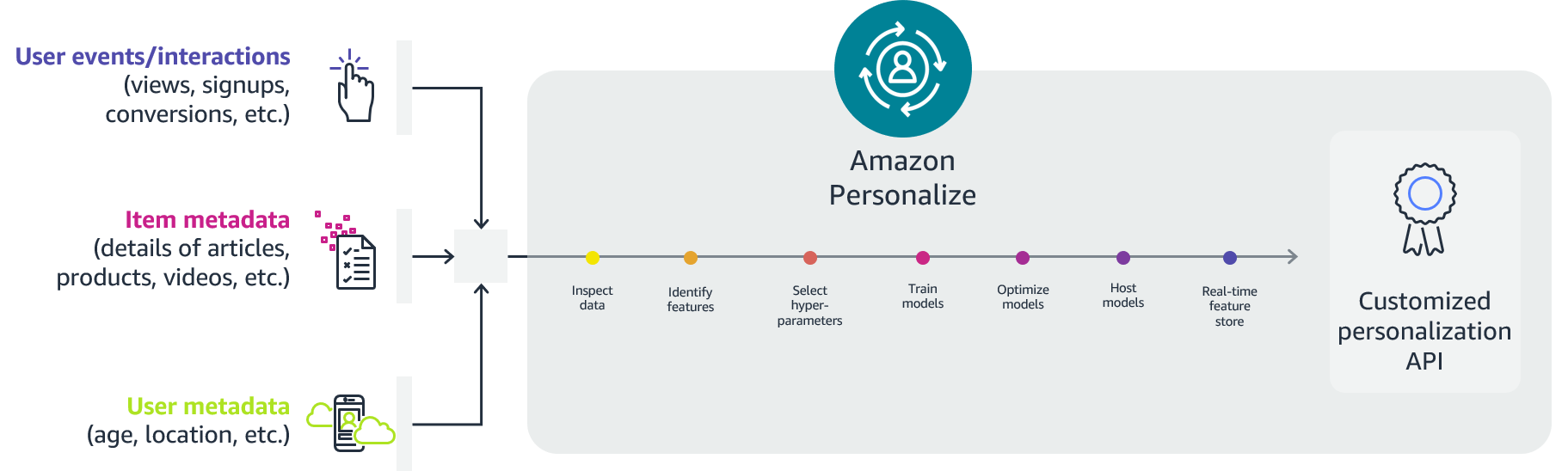
To make the ordering process more deterministic and to cater to peak demand times, The Chefz team decided to divide the day into different periods. For example, during Ramadan season, days are divided into Iftar and Suhoor. On regular days, days consist of four periods: breakfast, lunch, dinner, and dessert. The technology that underpins this deterministic ordering process is Amazon Personalize, a powerful recommendation engine. Amazon Personalize takes these grouped periods along with the location of the customer to provide a perfect recommendation.
This ensures the customer receives restaurant and meal recommendations based on their preference and from a nearby location so that it arrives quickly at their doorstep.
This recommendation engine based on Amazon Personalize is the key ingredient in how The Chefz’s customers enjoy personalized restaurant meal recommendations, rather than random recommendations for categories of favorites.
The personalization journey
The Chefz started its personalization journey by offering restaurant recommendations for customers using Amazon Personalize based on previous interactions, user metadata (such as age, nationality, and diet), restaurant metadata like category and food types offered, along with live tracking for customer interactions on the Chefz mobile application and web portal. The initial deployment phases of Amazon Personalize led to a 10% increase in customer interactions with the portal.
Although that was a milestone step, delivery time was still a problem that many customers encountered. One of the main difficulties customers had was delivery time during rush hour. To address this, the data scientist team added location as an additional feature to user metadata so recommendations would take into consideration both user preference and location for improved delivery time.
The next step in the recommendation journey was to consider annual timing, especially Ramadan, and the time of day. These considerations ensured The Chefz could recommend heavy meals or restaurants that provide Iftaar meals during Ramadan sundown, and lighter meals in the late evening. To solve this challenge, the data scientist team used Amazon Personalize filters updated by AWS Lambda functions, which were triggered by an Amazon CloudWatch cron job.
The following architecture shows the automated process for applying the filters:
- A CloudWatch event uses a cron expression to schedule when a Lambda function is invoked.
- When the Lambda function is triggered, it attaches the filter to the recommendation engine to apply business rules.
- Recommended meals and restaurants are delivered to end-users on the application.

Conclusion
Amazon Personalize enabled The Chefz to apply context about individual customers and their circumstances, and deliver customized recommendations based on business rules such as special deals and offers through our mobile application. This increased revenue by 35% per month and doubled customer orders at recommended restaurants.
“The customer is at the heart of everything we do at The Chefz, and we’re working tirelessly to improve and enhance their experience. With Amazon Personalize, we are able to achieve personalization at scale across our entire customer base, which was previously impossible.”
-Ramzi Algrainy, CTO at The Chefz.
About the authors
 Ramzi Alqrainy is Chief Technology Officer at The Chefz. Ramzi is a contributor to Apache Solr and Slack and technical reviewer, and has published many papers in IEEE focusing on search and data functions.
 Mohamed Ezzat is a Senior Solutions Architect at AWS with a focus in machine learning. He works with customers to address their business challenges using cloud technologies. Outside of work, he enjoys playing table tennis.
Distributed training with Amazon EKS and Torch Distributed Elastic
Distributed deep learning model training is becoming increasingly important as data sizes are growing in many industries. Many applications in computer vision and natural language processing now require training of deep learning models, which are growing exponentially in complexity and are often trained with hundreds of terabytes of data. It then becomes important to use a vast cloud infrastructure to scale the training of such large models.
Developers can use open-source frameworks such as PyTorch to easily design intuitive model architectures. However, scaling the training of these models across multiple nodes can be challenging due to increased orchestration complexity.
Distributed model training mainly consists of two paradigms:
- Model parallel – In model parallel training, the model itself is so large that it can’t fit in the memory of a single GPU, and multiple GPUs are needed to train the model. The Open AI’s GPT-3 model with 175 billion trainable parameters (approximately 350 GB in size) is a good example of this.
- Data parallel – In data parallel training, the model can reside in a single GPU, but because the data is so large, it can take days or weeks to train a model. Distributing the data across multiple GPU nodes can significantly reduce the training time.
In this post, we provide an example architecture to train PyTorch models using the Torch Distributed Elastic framework in a distributed data parallel fashion using Amazon Elastic Kubernetes Service (Amazon EKS).
Prerequisites
To replicate the results reported in this post, the only prerequisite is an AWS account. In this account, we create an EKS cluster and an Amazon FSx for Lustre file system. We also push container images to an Amazon Elastic Container Registry (Amazon ECR) repository in the account. Instructions to set up these components are provided as needed throughout the post.
EKS clusters
Amazon EKS is a managed container service to run and scale Kubernetes applications on AWS. With Amazon EKS, you can efficiently run distributed training jobs using the latest Amazon Elastic Compute Cloud (Amazon EC2) instances without needing to install, operate, and maintain your own control plane or nodes. It is a popular orchestrator for machine learning (ML) and AI workflows. A typical EKS cluster in AWS looks like the following figure.

We have released an open-source project, AWS DevOps for EKS (aws-do-eks), which provides a large collection of easy-to-use and configurable scripts and tools to provision EKS clusters and run distributed training jobs. This project is built following the principles of the Do Framework: Simplicity, Flexibility, and Universality. You can configure your desired cluster by using the eks.conf file and then launch it by running the eks-create.sh script. Detailed instructions are provided in the GitHub repo.
Train PyTorch models using Torch Distributed Elastic
Torch Distributed Elastic (TDE) is a native PyTorch library for training large-scale deep learning models where it’s critical to scale compute resources dynamically based on availability. The TorchElastic Controller for Kubernetes is a native Kubernetes implementation for TDE that automatically manages the lifecycle of the pods and services required for TDE training. It allows for dynamically scaling compute resources during training as needed. It also provides fault-tolerant training by recovering jobs from node failure.
In this post, we discuss the steps to train PyTorch EfficientNet-B7 and ResNet50 models using ImageNet data in a distributed fashion with TDE. We use the PyTorch DistributedDataParallel API and the Kubernetes TorchElastic controller, and run our training jobs on an EKS cluster containing multiple GPU nodes. The following diagram shows the architecture diagram for this model training.
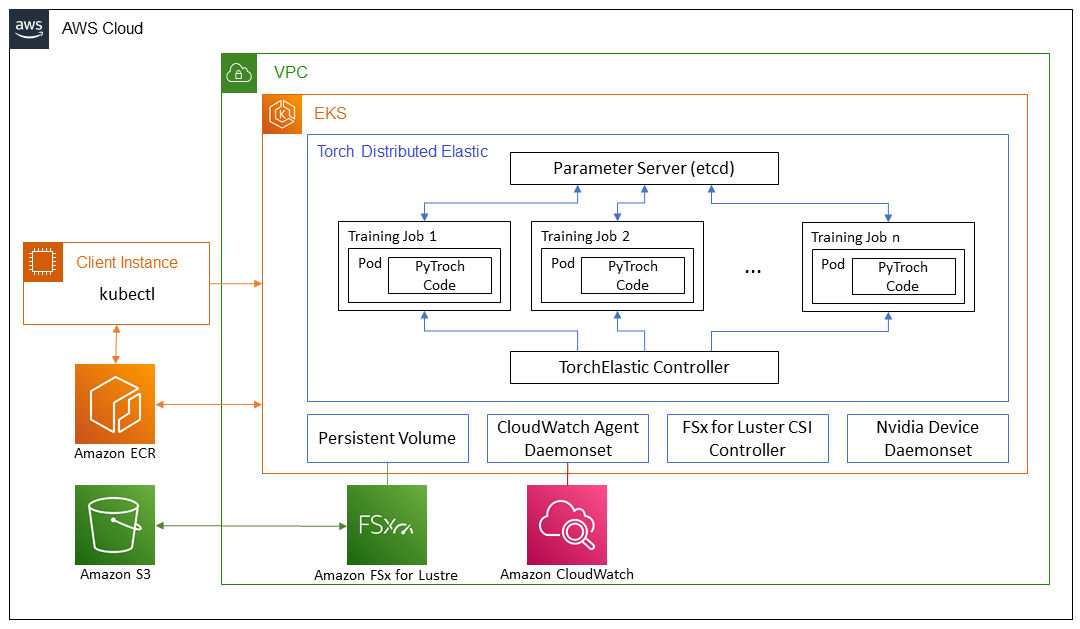
TorchElastic for Kubernetes consists mainly of two components: the TorchElastic Kubernetes Controller (TEC) and the parameter server (etcd). The controller is responsible for monitoring and managing the training jobs, and the parameter server keeps track of the worker nodes for distributed synchronization and peer discovery.
In order for the training pods to access the data, we need a shared data volume that can be mounted by each pod. Some options for shared volumes through Container Storage Interface (CSI) drivers included in AWS DevOps for EKS are Amazon Elastic File System (Amazon EFS) and FSx for Lustre.
Cluster setup
In our cluster configuration, we use one c5.2xlarge instance for system pods. We use three p4d.24xlarge instances as worker pods to train an EfficientNet model. For ResNet50 training, we use p3.8xlarge instances as worker pods. Additionally, we use an FSx shared file system to store our training data and model artifacts.
AWS p4d.24xlarge instances are equipped with Elastic Fabric Adapter (EFA) to provide networking between nodes. We discuss EFA more later in the post. To enable communication through EFA, we need to configure the cluster setup through a .yaml file. An example file is provided in the GitHub repository.
After this .yaml file is properly configured, we can launch the cluster using the script provided in the GitHub repo:
Refer to the GitHub repo for detailed instructions.
There is practically no difference between running jobs on p4d.24xlarge and p3.8xlarge. The steps described in this post work for both. The only difference is the availability of EFA on p4d.24xlarge instances. For smaller models like ResNet50, standard networking compared to EFA networking has minimal impact on the speed of training.
FSx for Lustre file system
FSx is designed for high-performance computing workloads and provides sub-millisecond latency using solid-state drive storage volumes. We chose FSx because it provided better performance as we scaled to a large number of nodes. An important detail to note is that FSx can only exist in a single Availability Zone. Therefore, all nodes accessing the FSx file system should exist in the same Availability Zone as the FSx file system. One way to achieve this is to specify the relevant Availability Zone in the cluster .yaml file for the specific node groups before creating the cluster. Alternatively, we can modify the network part of the auto scaling group for these nodes after the cluster is set up, and limit it to using a single subnet. This can be easily done on the Amazon EC2 console.
Assuming that the EKS cluster is up and running, and the subnet ID for the Availability Zone is known, we can set up an FSx file system by providing the necessary information in the fsx.conf file as described in the readme and running the deploy.sh script in the fsx folder. This sets up the correct policy and security group for accessing the file system. The script also installs the CSI driver for FSx as a daemonset. Finally, we can create the FSx persistent volume claim in Kubernetes by applying a single .yaml file:
This creates an FSx file system in the Availability Zone specified in the fsx.conf file, and also creates a persistent volume claim fsx-pvc, which can be mounted by any of the pods in the cluster in a read-write-many (RWX) fashion.
In our experiment, we used complete ImageNet data, which contains more that 12 million training images divided into 1,000 classes. The data can be downloaded from the ImageNet website. The original TAR ball has several directories, but for our model training, we’re only interested in ILSVRC/Data/CLS-LOC/, which includes the train and val subdirectories. Before training, we need to rearrange the images in the val subdirectory to match the directory structure required by the PyTorch ImageFolder class. This can be done using a simple Python script after the data is copied to the persistent volume in the next step.
To copy the data from an Amazon Simple Storage Service (Amazon S3) bucket to the FSx file system, we create a Docker image that includes scripts for this task. An example Dockerfile and a shell script are included in the csi folder within the GitHub repo. We can build the image using the build.sh script and then push it to Amazon ECR using the push.sh script. Before using these scripts, we need to provide the correct URI for the ECR repository in the .env file in the root folder of the GitHub repo. After we push the Docker image to Amazon ECR, we can launch a pod to copy the data by applying the relevant .yaml file:
The pod automatically runs the script data-prep.sh to copy the data from Amazon S3 to the shared volume. Because the ImageNet data has more than 12 million files, the copy process takes a couple of hours. The Python script imagenet_data_prep.py is also run to rearrange the val dataset as expected by PyTorch.
Network acceleration
We can use Elastic Fabric Adapter (EFA) in combination with supported EC2 instance types to accelerate network traffic between the GPU nodes in your cluster. This can be useful when running large distributed training jobs where standard network communication may be a bottleneck. Scripts to deploy and test the EFA device plugin in the EKS cluster that we use here are included in the efa-device-plugin folder in the GitHub repo. To enable a job with EFA in your EKS cluster, in addition to the cluster nodes having the necessary hardware and software, the EFA device plugin needs to be deployed to the cluster, and your job container needs to have compatible CUDA and NCCL versions installed.
To demonstrate running NCCL tests and evaluating the performance of EFA on p4d.24xlarge instances, we first must deploy the Kubeflow MPI operator by running the corresponding deploy.sh script in the mpi-operator folder. Then we run the deploy.sh script and update the test-efa-nccl.yaml manifest so limits and requests for resource vpc.amazonaws.com are set to 4. The four available EFA adapters in the p4d.24xlarge nodes get bundled together to provide maximum throughput.
Run kubectl apply -f ./test-efa-nccl.yaml to apply the test and then display the logs of the test pod. The following line in the log output confirms that EFA is being used:
The test results should look similar to the following output:
We can observe in the test results that the max throughput is about 42 GB/sec and average bus bandwidth is approximately 8 GB.
We also conducted experiments with a single EFA adapter enabled as well as no EFA adapters. All results are summarized in the following table.
| Number of EFA Adapters | Net/OFI Selected Provider | Avg. Bandwidth (GB/s) | Max. Bandwith (GB/s) |
| 4 | efa | 8.24 | 42.04 |
| 1 | efa | 3.02 | 5.89 |
| 0 | socket | 0.97 | 2.38 |
We also found that for relatively small models like ImageNet, the use of accelerated networking reduces the training time per epoch only with 5–8% at batch size of 64. For larger models and smaller batch sizes, when increased network communication of weights is needed, the use of accelerated networking has greater impact. We observed a decrease of epoch training time with 15–18% for training of EfficientNet-B7 with batch size 1. The actual impact of EFA on your training will depend on the size of your model.
GPU monitoring
Before running the training job, we can also set up Amazon CloudWatch metrics to visualize the GPU utilization during training. It can be helpful to know whether the resources are being used optimally or potentially identify resource starvation and bottlenecks in the training process.
The relevant scripts to set up CloudWatch are located in the gpu-metrics folder. First, we create a Docker image with amazon-cloudwatch-agent and nvidia-smi. We can use the Dockerfile in the gpu-metrics folder to create this image. Assuming that the ECR registry is already set in the .env file from the previous step, we can build and push the image using build.sh and push.sh. After this, running the deploy.sh script automatically completes the setup. It launches a daemonset with amazon-cloudwatch-agent and pushes various metrics to CloudWatch. The GPU metrics appear under the CWAgent namespace on the CloudWatch console. The rest of the cluster metrics show under the ContainerInsights namespace.
Model training
All the scripts needed for PyTorch training are located in the elasticjob folder in the GitHub repo. Before launching the training job, we need to run the etcd server, which is used by the TEC for worker discovery and parameter exchange. The deploy.sh script in the elasticjob folder does exactly that.
To take advantage of EFA in p4d.24xlarge instances, we need to use a specific Docker image available in the Amazon ECR Public Gallery that supports NCCL communication through EFA. We just need to copy our training code to this Docker image. The Dockerfile under the samples folder creates an image to be used when running training job on p4d instances. As always, we can use the build.sh and push.sh scripts in the folder to build and push the image.
The imagenet-efa.yaml file describes the training job. This .yaml file sets up the resources needed for running the training job and also mounts the persistent volume with the training data set up in the previous section.
A couple of things are worth pointing out here. The number of replicas should be set to the number of nodes available in the cluster. In our case, we set this to 3 because we had three p4d.24xlarge nodes. In the imagenet-efa.yaml file, the nvidia.com/gpu parameter under resources and nproc_per_node under args should be set to the number of GPUs per node, which in the case of p4d.24xlarge is 8. Also, the worker argument for the Python script sets the number of CPUs per process. We chose this to be 4 because, in our experiments, this provides optimal performance when running on p4d.24xlarge instances. These settings are necessary in order to maximize the use of all the hardware resources available in the cluster.
When the job is running, we can observe the GPU usage in CloudWatch for all the GPUs in the cluster. The following is an example from one of our training jobs with three p4d.24xlarge nodes in the cluster. Here we’ve selected one GPU from each node. With the settings mentioned earlier, the GPU usage is close to 100% during the training phase of the epoch for all of the nodes in the cluster.

For training a ResNet50 model using p3.8xlarge instances, we need exactly the same steps as described for the EfficientNet training using p4d.24xlarge. We can also use the same Docker image. As mentioned earlier, p3.8xlarge instances aren’t equipped with EFA. However, for the ResNet50 model, this is not a significant drawback. The imagenet-fsx.yaml script provided in the GitHub repository sets up the training job with appropriate resources for the p3.8xlarge node type. The job uses the same dataset from the FSx file system.
GPU scaling
We ran some experiments to observe how the training time scales for the EfficientNet-B7 model by increasing the number of GPUs. To do this, we changed the number of replicas from 1 to 3 in our training .yaml file for each training run. We only observed the time for a single epoch while using the complete ImageNet dataset. The following figure shows the results for our GPU scaling experiment. The red dotted line represents how the training time should go down from a run using 8 GPUs by increasing the number of GPUs. As we can see, the scaling is quite close to what is expected.

Similarly, we obtained the GPU scaling plot for ResNet50 training on p3.8xlarge instances. For this case, we changed the replicas in our .yaml file from 1 to 4. The results of this experiment are shown in the following figure.

Clean up
It’s important to spin down resources after model training in order to avoid costs associated with running idle instances. With each script that creates resources, the GitHub repo provides a matching script to delete them. To clean up our setup, we must delete the FSx file system before deleting the cluster because it’s associated with a subnet in the cluster’s VPC. To delete the FSx file system, we just need to run the following command (from inside the fsx folder):
Note that this will not only delete the persistent volume, it will also delete the FSx file system, and all the data on the file system will be lost. When this step is complete, we can delete the cluster by using the following script in the eks folder:
This will delete all the existing pods, remove the cluster, and delete the VPC created in the beginning.
Conclusion
In this post, we detailed the steps needed for running PyTorch distributed data parallel model training on EKS clusters. This task may seem daunting, but the AWS DevOps for EKS project created by the ML Frameworks team at AWS provides all the necessary scripts and tools to simplify the process and make distributed model training easily accessible.
For more information on the technologies used in this post, visit Amazon EKS and Torch Distributed Elastic. We encourage you to apply the approach described here to your own distributed training use cases.
Resources
- Amazon EC2 Instance Types
- Machine Learning on Amazon EKS
- Running TorchServe on Amazon Elastic Kubernetes Service
- Distributed Model Training Workshop for AWS EKS
About the authors
 Imran Younus is a Principal Solutions Architect for ML Frameworks team at AWS. He focuses on large scale machine learning and deep learning workloads across AWS services like Amazon EKS and AWS ParallelCluster. He has extensive experience in applications of Deep Leaning in Computer Vision and Industrial IoT. Imran obtained his PhD in High Energy Particle Physics where he has been involved in analyzing experimental data at peta-byte scales.
 Alex Iankoulski is a full-stack software and infrastructure architect who likes to do deep, hands-on work. He is currently a Principal Solutions Architect for Self-managed Machine Learning at AWS. In his role he focuses on helping customers with containerization and orchestration of ML and AI workloads on container-powered AWS services. He is also the author of the open source Do framework and a Docker captain who loves applying container technologies to accelerate the pace of innovation while solving the world’s biggest challenges. During the past 10 years, Alex has worked on combating climate change, democratizing AI and ML, making travel safer, healthcare better, and energy smarter.
Long-term Dynamics of Fairness Intervention in Connection Recommender Systems
Figure 1: Modeled recommendation cycle. We demonstrate how enforcing group-fairness in every recommendation slate separately does not necessarily promote equity in second order variables of interest like network size.
Connection recommendation is at the heart of user experience in many online social networks. Given a prompt such as ‘People you may know’, connection recommender systems suggest a list of users, and the recipient of the recommendation decides which of the users to connect with. In some instances, connection recommendations can account for more than 50% of the social network graph [1]. Depending on the platform, being connected to the right people is tied to important advantages such as job opportunities or increased visibility. While this makes it imperative to treat users fairly, it is far from obvious how fairness can be enforced or what it even means to have a ‘fair’ system in this scenario. In fact, when enforcing fairness in dynamic systems like this, we are often interested in second-order variables while interventions target equity in single steps [2]. In connection recommendation, this generally means enforcing some sort of parity condition in each recommendation slate, e.g. equal exposure of female and male users for every query, while simultaneously hoping that this will promote more equitable network sizes in the long run. In our work, we demonstrate how this approach can fail and common statistical notions of recommendation fairness do not ensure equity of network sizes in the long run. In fact, we see that fairness interventions are not even sufficient to mitigate the amplification of existing biases. We reach these conclusions based on an extensive simulation study supplemented by theoretical limit analyses. In the following, we focus on a discussion of empirical results and refer to the full paper for theoretical derivations.
Recommendation procedure
The assumed recommendation cycle is depicted in Figure 1. We briefly summarize the involved steps and give more detail on the most important components in the following sections. On the left in the flowchart, a user queries a connection recommendation, for example, by loading the ‘People You may Know’ page on the platform’s website. The system then computes relevance scores between the user who is seeking recommendations – which we will refer to as the source user – and other previously unconnected users who will be referred to as the destination users. Based on these relevance scores, we derive a ranking of destination users subject to fairness constraints and display a list of possible connections to the source user. After new connections have been made, the cycle repeats.
Fairness constrained probabilistic ranking framework
For each recommendation query, the system obtains a set of relevance scores and derives a probabilistic ranking. This probabilistic ranking takes the form of a matrix (P_{s,d}^q) where the entry in the (d)th row and (r)th column denotes the probability of displaying member (d) in slot (r) of the recommendation list. The probabilities are selected to maximize the expected utility for the source user which is common practice in the recommendation literature [3].
More formally, we denote the source member as (s) and the destination member as (d). (q) denotes a query for an ordered list of (m) destination members and (u_{s,d}^q) the relevance score of (s) and (d) under query (q). We model a form of position bias by discounting the expected attention a recommended user receives based on how far down the list the recommendation, i.e. we define the exposure of slot (r) as (v(r)=1/log(r+1)). Given these quantities, the optimization problem for query (q) can be written as
$$argmax_{P}u_s^TP^q_sv$$
$$text{s.t.} sum_{i=1}^nP_s^q(d,i)leq 1 text{ for all } din[D_q],$$
$$sum_{i=1}^{D_q}P_s^q(i,r)=1text{ for all }rin[m],$$
$$0leq P_s^q(i,r)leq 1text{ for all }iin[D_q],jin[m].$$
The constraints in this problem ensure that each slot has a recommended user and each user can be recommended at most once in a given list. We explore two types of fairness constraints to add to this problem. First, we consider demographic parity of exposure which is a commonly suggested form of fairness in recommendations. It requires that groups receive expected exposure proportional to their population shares, i.e. for groups (G_0) and (G_1)
$$frac{1}{vert G_0vert}sum_{din G_0}sum_{r=1}^mP_s^q(d,r)v_r=frac{1}{vert G_1vert}sum_{din G_1}sum_{r=1}^mP_s^q(d,r)v_r.$$
Assume a setting in which there is no position bias (v), the population is split into 60% majority group and 40% minority group, and each recommendation list has 10 slots. In this setting, demographic parity of exposure requires (in expectation) that 6 of the recommended members belong to the majority group while 4 belong to the minority group in every recommendation list.
Second, we explore a dynamic parity of utility constraint. As opposed to the first constraint, this fairness measure does not only consider the exposure of groups but also the total utility that can be expected from the exposure, i.e. for two groups (G_0) and (G_1),
$$frac{1}{vert G_0vert}sum_{din G_0}u_{s,d}^qsum_{r=1}^mP_s^q(d,r)v_r=frac{1}{vert G_1vert}sum_{din G_1}u_{s,d}^qsum_{r=1}^mP_s^q(d,r)v_r.$$
On a high level, the constraint requires that the sum of relevance scores across groups is proportional to the population share of groups discounted by the exposure limitations posed by position bias. To understand what this means, let us consider the example setting from before with no position bias, a 60%/40% group split, and recommendation lists with 10 slots. Assume that all destination members of the majority group have a relevance score of 0.12 while all destination members of the minority group have a fixed relevance of 0.08. The probabilistic ranking fulfills dynamic parity of utility if the expected group-split in the recommendation list is 50%/50% because (0.5 * 10 * 0.12 = 0.6) and (0.5 * 10 * 0.08 = 0.4).
How do we model relevance scores?
Relevance scores usually model the probability of connection if recommended, a measure of downstream engagement or some mixture of the two. The exact models employed by social media platforms are usually proprietary, but we opt for a synthetic model in the form of logistic regression in three realistic features [4,5]. Assuming our prediction target is the probability of connection, we first use the source member’s network size. This is based on the assumption that users with larger networks are more likely to be proactive in connection forming as they are generally more active on the platform. Next, we assume that users with more common connections are more likely to connect. The common connections feature is rooted in social network literature where it is commonly referred to as triadic closure [e.g. 6,7]. Lastly, we make the assumption that users with similarities such as demographics, interests, education, workplace, etc. are more likely to connect. This follows the observation that individuals like to be connected to similar individuals commonly referred to as homophily in sociology and other social sciences [e.g. 8].
The main simulation procedure makes use of the relevance scoring model for user pairs as follows. We assume a fixed-size graph of evolving connections with two groups of members. 65% of members belong to an initially more connected majority group. First, we assume a ground truth model for matching scores by imposing ground-truth parameter values in the presented logistic regression function. We use this function to simulate a data set of recommendations and formed connections and use the synthetic data to train a logistic regression matching scores model.
Simulation procedure
We sample covariate vectors from group-dependent distributions for each member in the graph. These vectors will be used to compute the similarity between members which we set as negative Euclidean distance. The connections in the graph are initialized with a stochastic block model in which user pairs in the majority group are slightly more likely to connect than user pairs in the minority group and user pairs who belong to the same group are slightly more likely to connect than user pairs who belong to opposite groups. This models the initial advantage for majority group members we would expect to see in practice and accounts for homophily preferences. Given the initial specifications, we go through the previously described recommendation cycle for 2,500 timesteps and keep track of key fairness and performance metrics. Following our reasoning from the scoring model, the frequency with which users seek out recommendations is based on exponential waiting times with a mean depending on the current network size of a user. The whole simulation procedure is repeated with each fairness intervention separately and without intervention for comparison. Results are averaged over 10 runs.
Rich-gets-richer in groups
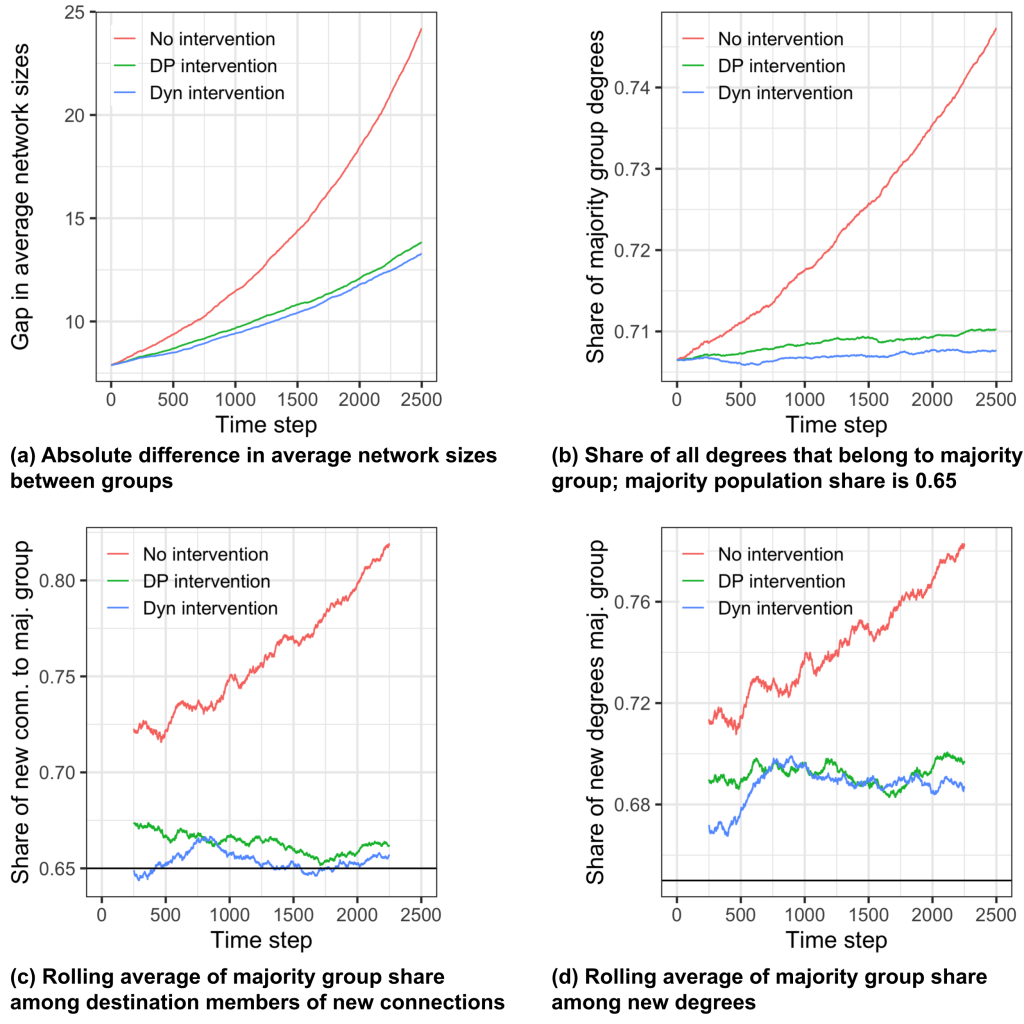
Figure 2 depicts the performance of all 3 intervention types. With no intervention – which is displayed in red in the graphs – we observe that the gap in average network sizes between groups drastically increases over time. In fact, our results reveal a group-wise rich-get-richer effect in which network sizes tend to a power law distribution with a lower mode in the minority population. Members whose networks are in the tail of the distribution tend to be the members who had large networks, as compared to their peers, to begin with. These observations are in line with previous findings on rich-get-richer phenomena under homophily.
Demographic parity of exposure intervention
We now move to the results for the demographic parity of exposure intervention. First, we can see that the majority group share of exposure in recommendations is down to 66.3% which suggests that the intervention is working. However, as we can see in panels (a) and (b), the gap in average network sizes is still increasing over time. Why is this the case? First, majority group members seek out recommendations more frequently based on their already larger network sizes and activity levels. This leads to more connections formed with majority group members at the source side of the recommendation while our intervention can only target the destination side. Second, majority group members have higher ranking scores and are thus more likely to be invited for connection even if both groups are exposed equally. Consider the following example recommendation:
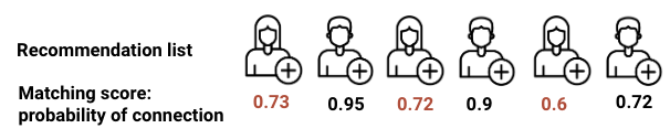
Here, both female and male users have the same exposure – we will ignore position bias for this example. However, the probability of connection and its proxy – the matching score – are much lower for women than for men essentially leading to fewer new connections for women than for men. While the intervention suggests recommendations are made fairly, this does not align with our intuitive goal of more equitable network sizes.
Dynamic parity of utility intervention
Some of the problems with the demographic parity of exposure intervention are addressed by the dynamic parity of utility intervention. We see that the majority group share of destination members of new connections is down to 65.4% as desired. Yet, even with this type of constraint, panels (a) and (b) show that the gap in average network sizes is still increasing over time. Like in the previous case, one of the reasons for this is that majority group members seek out recommendations more frequently. In addition, our analysis reveals that source members from the majority group generally form more connections per recommendation query leading to the increased share in panel (d). To understand why this is the case, consider the following example:
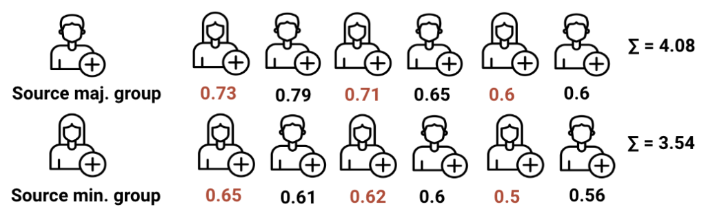
In the first row, a majority group member – here displayed as male – receives recommendations. In the second row, a minority group member – here female – receives recommendations. In both recommendation lists the dynamic parity of utility constraint is fulfilled, but the male source member receives more overall utility from the query because the constraint can only target fairness within a list and not in between different sets of recommendations.
Summary of findings
Let us summarize the key findings. Our study shows that unconstrained connection recommendation leads to a group-wise rich-get-richer effect. Enforcing demographic parity of exposure or dynamic parity of utility between groups, which are commonly suggested remedies against demographic bias in recommender systems, leads to less bias amplification but is not sufficient in order to mitigate an increase in the disparities in network sizes over time. As shown in the full paper, theoretical limit analysis shows that dynamic parity of utility would be the optimal intervention if there was no source-side bias. Yet, this is an unrealistic assumption in practice.
Overall, the common practice of measuring fairness in recommender systems in a one-shot or time-aggregate static manner can lead to an illusion of fairness and deployment of fairness-enhancing algorithms with unforeseen consequences. Connection recommendation operates on a dynamical system that needs to be taken into account to ensure equitable outcomes in the long run.
The full paper is published in the proceedings of the AAAI / ACM conference on Artificial Intelligence, Ethics, and Society (AIES 2022). A preprint is available here.
References
[1] LinkedIn PYMK: https://engineering.linkedin.com/teams/data/artificial-intelligence/people-you-may-know [Online; accessed 7/6/22] [2] Lydia T. Liu, Sarah Dean, Esther Rolf, Max Simchowitz, and Moritz Hardt. Delayed impact of fair machine learning. In Proceedings of the 35th International Conference on Machine Learning (ICLM 2018), 2018. [3] Deepak K. Agarwal and Bee-Chung Chen. 2016. Statistical Methods for Recommender Systems. Cambridge University Press. [4] LinkedIn PYMK: https://engineering.linkedin.com/teams/data/artificial-intelligence/people-you-may-know [Online; accessed 7/6/22] [5] Facebook PYMK: https://www.facebook.com/help/336320879782850 [Online; accessed 7/6/22] [6] Kossinets, G., & Watts, D. J. (2006). Empirical Analysis of an Evolving Social Network. In Science (Vol. 311, Issue 5757, pp. 88–90). American Association for the Advancement of Science (AAAS). [7] David Liben-Nowell and Jon Kleinberg. 2007. The link-prediction problem for social networks. J. Am. Soc. Inf. Sci. Technol. 58, 7 (May 2007), 1019–1031. [8] McPherson, M., Smith-Lovin, L., & Cook, J. M. (2001). Birds of a Feather: Homophily in Social Networks. In Annual Review of Sociology (Vol. 27, Issue 1, pp. 415–444). Annual Reviews.Model assesses the validity of tips offered in product reviews
Method would enable customers to evaluate supporting evidence for tip reliability.Read More
Using machine learning to identify undiagnosable cancers
The first step in choosing the appropriate treatment for a cancer patient is to identify their specific type of cancer, including determining the primary site — the organ or part of the body where the cancer begins.
In rare cases, the origin of a cancer cannot be determined, even with extensive testing. Although these cancers of unknown primary tend to be aggressive, oncologists must treat them with non-targeted therapies, which frequently have harsh toxicities and result in low rates of survival.
A new deep-learning approach developed by researchers at the Koch Institute for Integrative Cancer Research at MIT and Massachusetts General Hospital (MGH) may help classify cancers of unknown primary by taking a closer look the gene expression programs related to early cell development and differentiation.
“Sometimes you can apply all the tools that pathologists have to offer, and you are still left without an answer,” says Salil Garg, a Charles W. (1955) and Jennifer C. Johnson Clinical Investigator at the Koch Institute and a pathologist at MGH. “Machine learning tools like this one could empower oncologists to choose more effective treatments and give more guidance to their patients.”
Garg is the senior author of a new study, published Aug. 30 in Cancer Discovery, and MIT postdoc Enrico Moiso is the lead author. The artificial intelligence tool is capable of identifying cancer types with a high degree of sensitivity and accuracy.
Machine learning in development
Parsing the differences in the gene expression among different kinds of tumors of unknown primary is an ideal problem for machine learning to solve. Cancer cells look and behave quite differently from normal cells, in part because of extensive alterations to how their genes are expressed. Thanks to advances in single cell profiling and efforts to catalog different cell expression patterns in cell atlases, there are copious — if, to human eyes, overwhelming — data that contain clues to how and from where different cancers originated.
However, building a machine learning model that leverages differences between healthy and normal cells, and among different kinds of cancer, into a diagnostic tool is a balancing act. If a model is too complex and accounts for too many features of cancer gene expression, the model may appear to learn the training data perfectly, but falter when it encounters new data. However, by simplifying the model by narrowing the number of features, the model may miss the kinds of information that would lead to accurate classifications of cancer types.
In order to strike a balance between reducing the number of features while still extracting the most relevant information, the team focused the model on signs of altered developmental pathways in cancer cells. As an embryo develops and undifferentiated cells specialize into various organs, a multitude of pathways directs how cells divide, grow, change shape, and migrate. As the tumor develops, cancer cells lose many of the specialized traits of a mature cell. At the same time, they begin to resemble embryonic cells in some ways, as they gain the ability to proliferate, transform, and metastasize to new tissues. Many of the gene expression programs that drive embryogenesis are known to be reactivated or dysregulated in cancer cells.
The researchers compared two large cell atlases, identifying correlations between tumor and embryonic cells: the Cancer Genome Atlas (TCGA), which contains gene expression data for 33 tumor types, and the Mouse Organogenesis Cell Atlas (MOCA), which profiles 56 separate trajectories of embryonic cells as they develop and differentiate.
“Single-cell resolution tools have dramatically changed how we study the biology of cancer, but how we make this revolution impactful for patients is another question,” explains Moiso. “With the emergence of developmental cell atlases, especially ones that focus on early phases of organogenesis such as MOCA, we can expand our tools beyond histological and genomic information and open doors to new ways of profiling and identifying tumors and developing new treatments.”
The resulting map of correlations between developmental gene expression patterns in tumor and embryonic cells was then transformed into a machine learning model. The researchers broke down the gene expression of tumor samples from the TCGA into individual components that correspond to a specific point of time in a developmental trajectory, and assigned each of these components a mathematical value. The researchers then built a machine-learning model, called the Developmental Multilayer Perceptron (D-MLP), that scores a tumor for its developmental components and then predicts its origin.
Classifying tumors
After training, the D-MLP was applied to 52 new samples of particularly challenging cancers of unknown primary that could not be diagnosed using available tools. These cases represented the most challenging seen at MGH over a four-year period beginning in 2017. Excitingly, the model classed the tumors to four categories, and yielded predictions and other information that could guide diagnosis and treatment of these patients.
For example, one sample came from a patient with a history of breast cancer who showed signs of an aggressive cancer in the fluid spaces around the abdomen. Oncologists initially could not find a tumor mass, and could not classify cancer cells using the tools they had at the time. However, the D-MLP strongly predicted ovarian cancer. Six months after the patient first presented, a mass was finally found in the ovary that proved to be the origin of tumor.
Moreover, the study’s systematic comparisons between tumor and embryonic cells revealed promising, and sometimes surprising, insights into the gene expression profiles of specific tumor types. For instance, in early stages of embryonic development, a rudimentary gut tube forms, with the lungs and other nearby organs arising from the foregut, and much of the digestive tract forming from the mid- and hindgut. The study showed that lung-derived tumor cells showed strong similarities not just to the foregut as might be expected, but to the to mid- and hindgut-derived developmental trajectories. Findings like these suggest that differences in developmental programs could one day be exploited in the same way that genetic mutations are commonly used to design personalized or targeted cancer treatments.
While the study presents a powerful approach to classifying tumors, it has some limitations. In future work, researchers plan to increase the predictive power of their model by incorporating other types of data, notably information gleaned from radiology, microscopy, and other types of tumor imaging.
“Developmental gene expression represents only one small slice of all the factors that could be used to diagnose and treat cancers,” says Garg. “Integrating radiology, pathology, and gene expression information together is the true next step in personalized medicine for cancer patients.”
This study was funded, in part, by the Koch Institute Support (core) Grant from the National Cancer Institute and by the National Cancer Institute.
Using machine learning to identify undiagnosable cancers
The first step in choosing the appropriate treatment for a cancer patient is to identify their specific type of cancer, including determining the primary site — the organ or part of the body where the cancer begins.
In rare cases, the origin of a cancer cannot be determined, even with extensive testing. Although these cancers of unknown primary tend to be aggressive, oncologists must treat them with non-targeted therapies, which frequently have harsh toxicities and result in low rates of survival.
A new deep-learning approach developed by researchers at the Koch Institute for Integrative Cancer Research at MIT and Massachusetts General Hospital (MGH) may help classify cancers of unknown primary by taking a closer look the gene expression programs related to early cell development and differentiation.
“Sometimes you can apply all the tools that pathologists have to offer, and you are still left without an answer,” says Salil Garg, a Charles W. (1955) and Jennifer C. Johnson Clinical Investigator at the Koch Institute and a pathologist at MGH. “Machine learning tools like this one could empower oncologists to choose more effective treatments and give more guidance to their patients.”
Garg is the senior author of a new study, published Aug. 30 in Cancer Discovery. The artificial intelligence tool is capable of identifying cancer types with a high degree of sensitivity and accuracy. Garg is the senior author of the study, and MIT postdoc Enrico Moiso is the lead author.
Machine learning in development
Parsing the differences in the gene expression among different kinds of tumors of unknown primary is an ideal problem for machine learning to solve. Cancer cells look and behave quite differently from normal cells, in part because of extensive alterations to how their genes are expressed. Thanks to advances in single cell profiling and efforts to catalog different cell expression patterns in cell atlases, there are copious — if, to human eyes, overwhelming — data that contain clues to how and from where different cancers originated.
However, building a machine learning model that leverages differences between healthy and normal cells, and among different kinds of cancer, into a diagnostic tool is a balancing act. If a model is too complex and accounts for too many features of cancer gene expression, the model may appear to learn the training data perfectly, but falter when it encounters new data. However, by simplifying the model by narrowing the number of features, the model may miss the kinds of information that would lead to accurate classifications of cancer types.
In order to strike a balance between reducing the number of features while still extracting the most relevant information, the team focused the model on signs of altered developmental pathways in cancer cells. As an embryo develops and undifferentiated cells specialize into various organs, a multitude of pathways directs how cells divide, grow, change shape, and migrate. As the tumor develops, cancer cells lose many of the specialized traits of a mature cell. At the same time, they begin to resemble embryonic cells in some ways, as they gain the ability to proliferate, transform, and metastasize to new tissues. Many of the gene expression programs that drive embryogenesis are known to be reactivated or dysregulated in cancer cells.
The researchers compared two large cell atlases, identifying correlations between tumor and embryonic cells: the Cancer Genome Atlas (TCGA), which contains gene expression data for 33 tumor types, and the Mouse Organogenesis Cell Atlas (MOCA), which profiles 56 separate trajectories of embryonic cells as they develop and differentiate.
“Single-cell resolution tools have dramatically changed how we study the biology of cancer, but how we make this revolution impactful for patients is another question,” explains Moiso. “With the emergence of developmental cell atlases, especially ones that focus on early phases of organogenesis such as MOCA, we can expand our tools beyond histological and genomic information and open doors to new ways of profiling and identifying tumors and developing new treatments.”
The resulting map of correlations between developmental gene expression patterns in tumor and embryonic cells was then transformed into a machine learning model. The researchers broke down the gene expression of tumor samples from the TCGA into individual components that correspond to a specific point of time in a developmental trajectory, and assigned each of these components a mathematical value. The researchers then built a machine-learning model, called the Developmental Multilayer Perceptron (D-MLP), that scores a tumor for its developmental components and then predicts its origin.
Classifying tumors
After training, the D-MLP was applied to 52 new samples of particularly challenging cancers of unknown primary that could not be diagnosed using available tools. These cases represented the most challenging seen at MGH over a four-year period beginning in 2017. Excitingly, the model classed the tumors to four categories, and yielded predictions and other information that could guide diagnosis and treatment of these patients.
For example, one sample came from a patient with a history of breast cancer who showed signs of an aggressive cancer in the fluid spaces around the abdomen. Oncologists initially could not find a tumor mass, and could not classify cancer cells using the tools they had at the time. However, the D-MLP strongly predicted ovarian cancer. Six months after the patient first presented, a mass was finally found in the ovary that proved to be the origin of tumor.
Moreover, the study’s systematic comparisons between tumor and embryonic cells revealed promising, and sometimes surprising, insights into the gene expression profiles of specific tumor types. For instance, in early stages of embryonic development, a rudimentary gut tube forms, with the lungs and other nearby organs arising from the foregut, and much of the digestive tract forming from the mid- and hindgut. The study showed that lung-derived tumor cells showed strong similarities not just to the foregut as might be expected, but to the to mid- and hindgut-derived developmental trajectories. Findings like these suggest that differences in developmental programs could one day be exploited in the same way that genetic mutations are commonly used to design personalized or targeted cancer treatments.
While the study presents a powerful approach to classifying tumors, it has some limitations. In future work, researchers plan to increase the predictive power of their model by incorporating other types of data, notably information gleaned from radiology, microscopy, and other types of tumor imaging.
“Developmental gene expression represents only one small slice of all the factors that could be used to diagnose and treat cancers,” says Garg. “Integrating radiology, pathology, and gene expression information together is the true next step in personalized medicine for cancer patients.”
This study was funded, in part, by the Koch Institute Support (core) Grant from the National Cancer Institute and by the National Cancer Institute.
NVIDIA GTC Dives Into the Industrial Metaverse, Digital Twins
This month’s NVIDIA GTC provides the best opportunity yet to learn how leading companies and their designers, planners and operators are using the industrial metaverse to create physically accurate, perfectly synchronized, AI-enabled digital twins.
The global conference, which runs online Sept. 19-22, will focus in part on how NVIDIA Omniverse Enterprise enables companies to design products, processes and facilities before bringing them to life in the real world — as well as simulate current and future operations.
Here are some of the experts — from such fields as retail, healthcare and manufacturing — who will discuss the of use AI-enabled digital twins:
- The Opportunity of the Industrial Metaverse, a panel discussion featuring Peggy Johnson, CEO of Magic Leap; Inga von Bibra, chief information officer of research and development at Mercedes Benz AG; Matthew Ball, CEO of Epyllion; Tony Hemmelgarn, CEO of Siemens Digital Industries Software; Dean Takahashi, lead writer at VentureBeat; and Rev Lebaredian, vice president of simulation technology and Omniverse engineering at NVIDIA.
- Lowe’s: Fully Digitizing the World of Home Improvement, a panel discussion featuring Cheryl Friedman, vice president, and Mason Sheffield, director of creative technology at Lowe’s Innovation Lab.
- Customer-Driven Grocery Enabled by NVIDIA AI at Kroger, a fireside chat featuring Wesley Rhodes, vice president of technology transformation and research and development at Kroger, and Azita Martin, vice president of AI for retail and consumer packaged goods at NVIDIA.
- Making Production More Sustainable With the Industrial Metaverse, a talk featuring Cedrik Neike, CEO of digital industries at Siemens AG.
- The Rise of Transformer AI and Digital Twins in Healthcare, a special address featuring Kimberly Powell, vice president of healthcare and life sciences at NVIDIA.
Other sessions feature Guido Quaroni, senior director of engineering at Adobe; Matt Sivertson, vice president and chief architect for media and entertainment at Autodesk; and Steve May, vice president and chief technology officer at Pixar.
Plus, learn how to build a digital twin with these introductory learning sessions:
- How to Build a Digital Twin: Full-Design Fidelity Visualization and Aggregation of 3D Data
- How to Build a Digital Twin: Bringing in Robotics
- Technical Breakout: How to Build a Digital Twin With NVIDIA Omniverse
For hands-on, instructor-led training workshops, check out sessions from the NVIDIA Deep Learning Institute. GTC offers a full day of learning on Monday, Sept. 19.
Register free for GTC and watch NVIDIA founder and CEO Jensen Huang’s keynote on Tuesday, Sept. 20, at 8 a.m. PT to hear about the latest technology breakthroughs.
Feature image courtesy of Amazon Robotics.
The post NVIDIA GTC Dives Into the Industrial Metaverse, Digital Twins appeared first on NVIDIA Blog.