A key challenge in many modern data analysis tasks is that user data is heterogeneous. Different users may possess vastly different numbers of data points. More importantly, it cannot be assumed that all users sample from the same underlying distribution. This is true, for example in language data, where different speech styles result in data heterogeneity. In this work we propose a simple model of heterogeneous user data that differs in both distribution and quantity of data, and we provide a method for estimating the population-level mean while preserving user-level differential privacy. We…Apple Machine Learning Research
Two-Layer Bandit Optimization for Recommendations
Online commercial app marketplaces serve millions of apps to billions of users in an efficient manner. Bandit optimization algorithms are used to ensure that the recommendations are relevant, and converge to the best performing content over time. However, directly applying bandits to real-world systems, where the catalog of items is dynamic and continuously refreshed, is not straightforward. One of the challenges we face is the existence of several competing content surfacing components, a phenomenon not unusual in large-scale recommender systems. This often leads to challenging scenarios…Apple Machine Learning Research
Index your Dropbox content using the Dropbox connector for Amazon Kendra
Amazon Kendra is a highly accurate and simple-to-use intelligent search service powered by machine learning (ML). Amazon Kendra offers a suite of data source connectors to simplify the process of ingesting and indexing your content, wherever it resides.
Valuable data in organizations is stored in both structured and unstructured repositories. An enterprise search solution should be able to pull together data across several structured and unstructured repositories to index and search on.
One such data repository is Dropbox. Enterprise users use Dropbox to upload, transfer, and store documents to the cloud. Along with the ability to store documents, Dropbox offers Dropbox Paper, a coediting tool that lets users collaborate and create content in one place. Dropbox Paper can optionally use templates to add structure to documents. In addition to files and paper, Dropbox also allows you to store shortcuts to webpages in your folders.
We’re excited to announce that you can now use the Amazon Kendra connector for Dropbox to search information stored in your Dropbox account. In this post, we show how to index information stored in Dropbox and use the Amazon Kendra intelligent search function. In addition, Amazon Kendra’s ML powered intelligent search can accurately find information from unstructured documents having natural language narrative content, for which keyword search is not very effective.
Solution overview
With Amazon Kendra, you can configure multiple data sources to provide a central place to search across your document repository. For our solution, we demonstrate how to index a Dropbox repository or folder using the Amazon Kendra connector for Dropbox. The solution consists of the following steps:
- Configure an app on Dropbox and get the connection details.
- Store the details in AWS Secrets Manager.
- Create a Dropbox data source via the Amazon Kendra console.
- Index the data in the Dropbox repository.
- Run a sample query to get the information.
Prerequisites
To try out the Amazon Kendra connector for Dropbox, you need the following:
- A Dropbox Enterprise (not personal) account.
- An AWS account with privileges to create AWS Identity and Access Management (IAM) roles and policies. For more information, see Overview of access management: Permissions and policies.
- Basic knowledge of AWS.
Configure a Dropbox app and gather connection details
Before we set up the Dropbox data source, we need a few details about your Dropbox repository. Let’s gather those in advance.
- Go to www.dropbox.com/developers.
- Choose App console.

- Sign in with your credentials (make sure you’re signing in to an Enterprise account).

- Choose Create app.

- Select Scoped access.
- Select Full Dropbox (or the name of the specific folder you want to index).
- Enter a name for your app.
- Choose Create app.

You can see the configuration screen with a set of tabs. - To set up permissions, choose the Permissions tab.
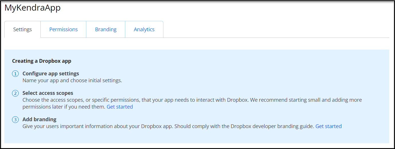
- Select a minimal set of permissions, as shown in the following screenshots.
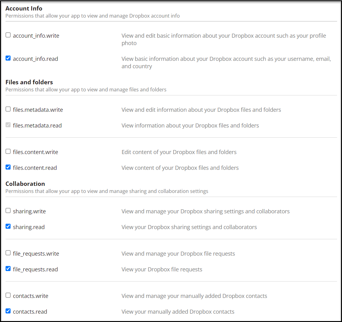


- Choose Submit.

A message appears saying that the permission change was successful.

- On the Settings tab, copy the app key.
- Choose Show next to App secret and copy the secret.
- Under Generated access token, choose Generate and copy the token.
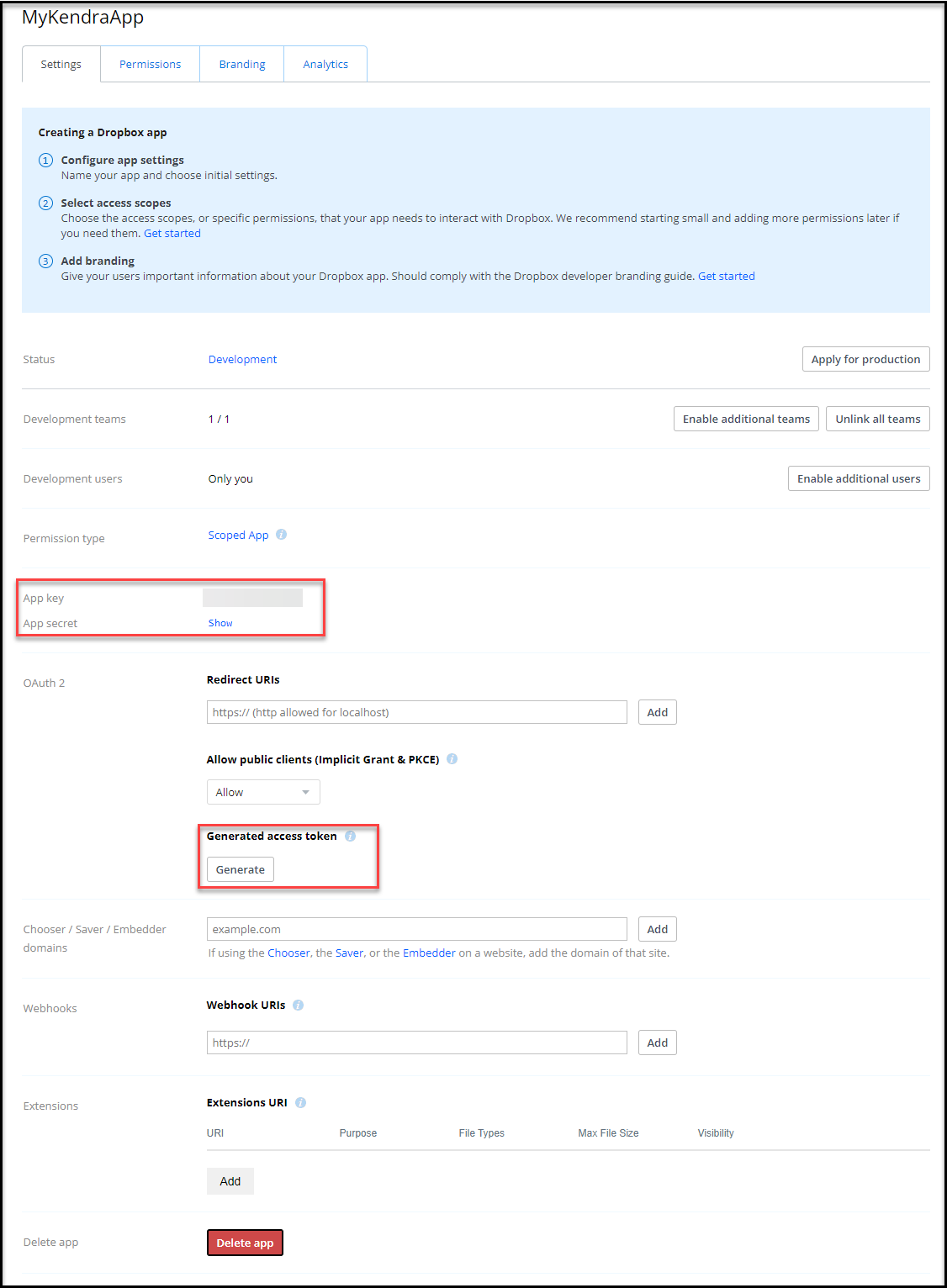
Store these values in a safe place—we need to refer to these later.
The session token is valid for up to 4 hours. You have to generate a new session token each time you index the content.
Store Dropbox credentials in Secrets Manager
To store your Dropbox credentials in Secrets Manager, compete the following steps:
- On the Secrets Manager console, choose Store a new secret.
- Choose Other type of secret.
- Create three key-value pairs for
appKey,appSecret, andrefreshTokenand enter the values saved from Dropbox. - Choose Save.

- For Secret name, enter a name (for example,
AmazonKendra-dropbox-secret). - Enter an optional description.
- Choose Next.

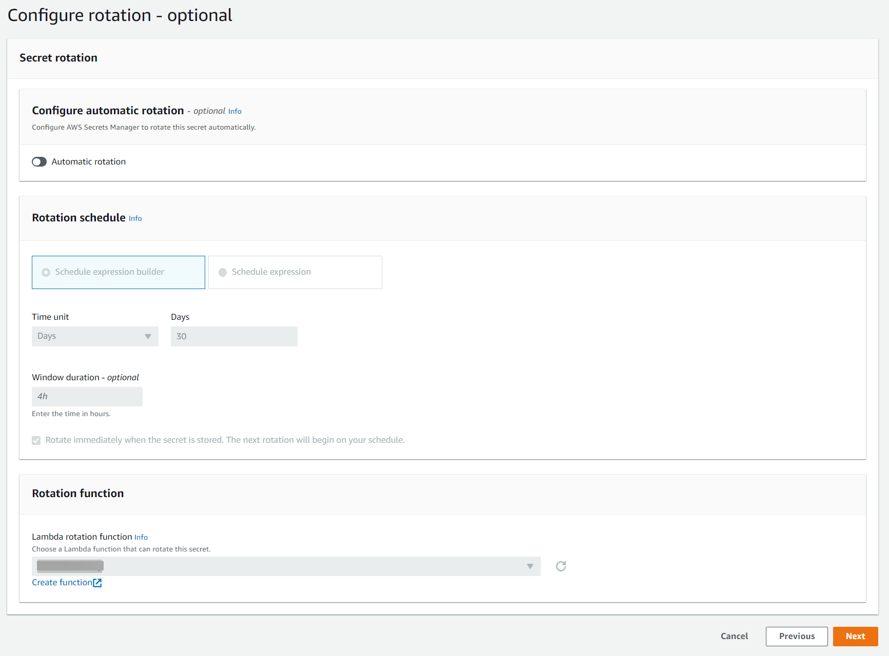
- In the Configure rotation section, keep all settings at their defaults and choose Next.
- On the Review page, choose Store.

Configure the Amazon Kendra connector for Dropbox
To configure the Amazon Kendra connector, complete the following steps:
- On the Amazon Kendra console, choose Create an Index.

- For Index name, enter a name for the index (for example,
my-dropbox-index). - Enter an optional description.
- For Role name, enter an IAM role name.
- Configure optional encryption settings and tags.
- Choose Next.

- In the Configure user access control section, leave the settings at their defaults and choose Next.

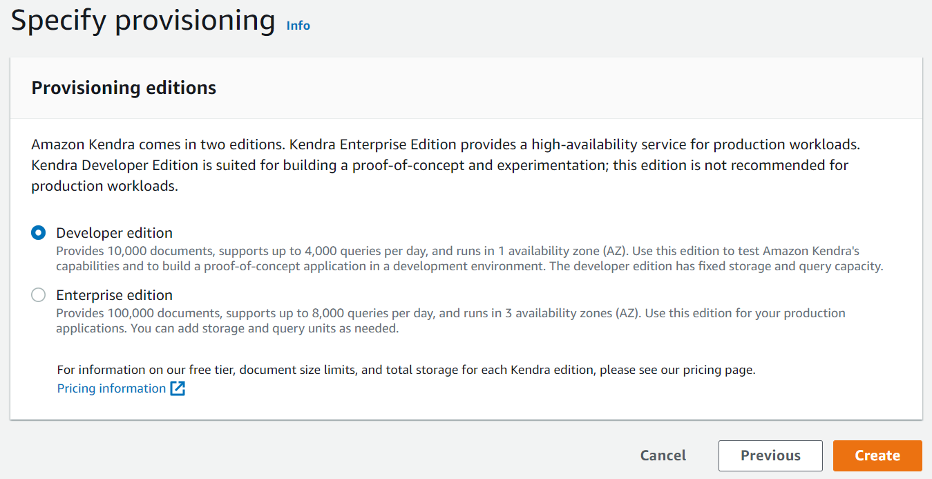
- For Provisioning editions, select Developer edition.
- Choose Create.
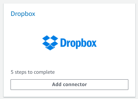
This creates and propagates the IAM role and then creates the Amazon Kendra index, which can take up to 30 minutes. - Choose Data sources in the navigation pane.

- Under Dropbox, choose Add connector.
- For Data source name, enter a name (for example,
my-dropbox-connector). - Enter an optional description.
- Choose Next.

- For Type of authentication token, select Access Token (temporary use).
- For AWS Secrets Manager secret, choose the secret you created earlier.
- For IAM role, choose Create a new role.
- For Role name, enter a name (for example,
AmazonKendra-dropbox-role). - Choose Next.

- For Select entities or content types, choose your content types.
- For Frequency, choose Run on demand.
- Choose Next.

- Set any optional field mappings and choose Next.
- Choose Review and Create and choose Add data source.
- Choose Sync now.

- Wait for the sync to complete.

Test the solution
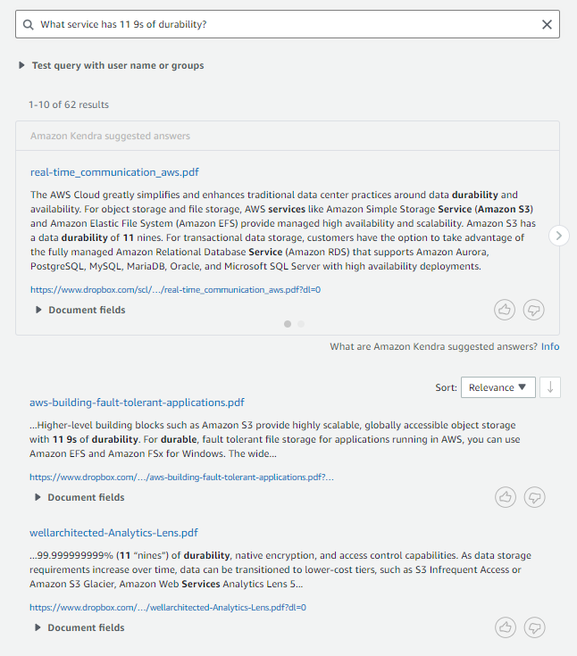
Now that you have ingested the content from your Dropbox account into your Amazon Kendra index, you can test some queries.
Go to your index and choose Search indexed content. Enter a sample search query and test out your search results (your query will vary based on the contents of your account).
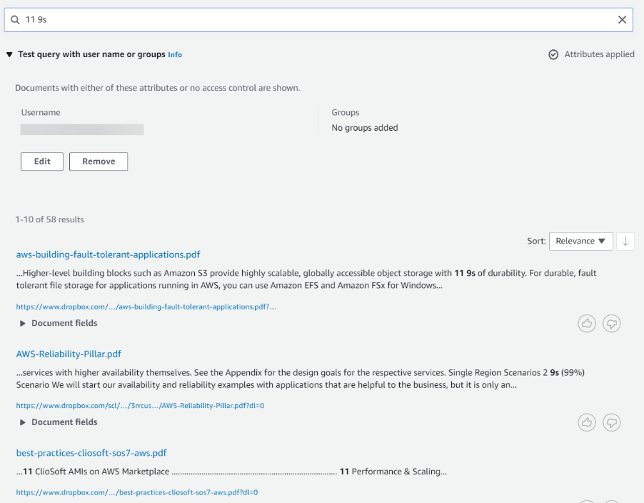
The Dropbox connector also crawls local identity information from Dropbox. For users, it sets user email id as principal. For groups, it sets group id as principal. To filter search results by users/groups, go to the Search Console.
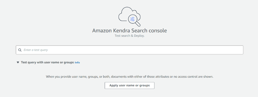
Click on “Test query with user name or groups” to expand it and click on the button that says “apply user name or groups”.
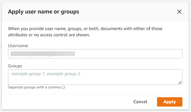
Enter the user and/or group names and click Apply. Next, enter the search query and hit enter. This brings you a filtered set of results based on your criteria.
Congratulations! You have successfully used Amazon Kendra to surface answers and insights based on the content indexed from your Dropbox account.
Generate permanent tokens for offline access
The instructions in this post walk you through creating, configuring, and using a temporary access token. Apps can also get long-term access by requesting offline access, in which case the app receives a refresh token that can be used to retrieve new short-lived access tokens as needed, without further manual user intervention. You can find more information in the Dropbox OAuth Guide and Dropbox authorization documentation. Use the following steps to create a permanent refresh token (for example to set the sync to trigger on a schedule):
- Get the app key and app secret as before.
- In a new browser, navigate to
https://www.dropbox.com/oauth2/authorize?token_access_type=offline&response_type=code&client_id=<appkey>. - Accept the defaults and choose Submit.
- Choose Continue.

- Choose Allow.

An access code is generated for you. - Copy the access code.

Now you get the refresh token from the access code. - In a terminal window, run the following curl command:
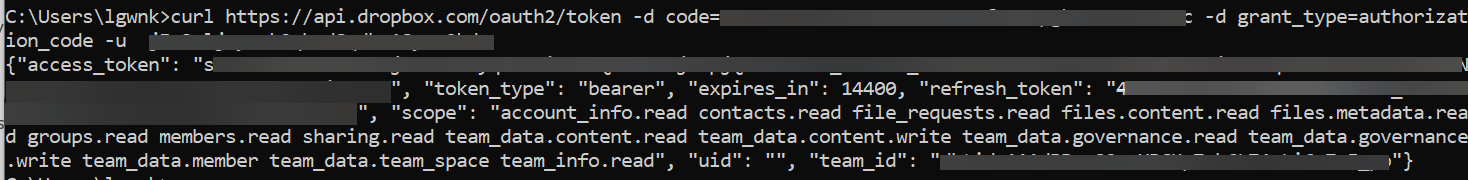
You can store this refresh token along with the app key and app secret to configure a permanent token in the data source configuration for Amazon Kendra. Amazon Kendra generates the access token and uses it as needed for access.
Limitations
This solution has the following limitations:
- File comments are not imported into the index
- You don’t have the option to add custom metadata for Dropbox
- Google docs, sheets, and slides need a Google workspace or Google account and are not included
Conclusion
With the Dropbox connector for Amazon Kendra, organizations can tap into the repository of information stored in their account securely using intelligent search powered by Amazon Kendra.
In this post, we introduced you to the basics, but there are many additional features that we didn’t cover. For example:
- You can enable user-based access control for your Amazon Kendra index and restrict access to users and groups that you configure
- You can specify
allowedUsersColumnandallowedGroupsColumnso you can apply access controls based on users and groups, respectively - You can map additional fields to Amazon Kendra index attributes and enable them for faceting, search, and display in the search results
- You can integrate the Dropbox data source with the Custom Document Enrichment (CDE) capability in Amazon Kendra to perform additional attribute mapping logic and even custom content transformation during ingestion
To learn about these possibilities and more, refer to the Amazon Kendra Developer Guide.
About the author
 Ashish Lagwankar is a Senior Enterprise Solutions Architect at AWS. His core interests include AI/ML, serverless, and container technologies. Ashish is based in the Boston, MA, area and enjoys reading, outdoors, and spending time with his family.

Neurodegenerative disease can progress in newly identified patterns
Neurodegenerative diseases — like amyotrophic lateral sclerosis (ALS, or Lou Gehrig’s disease), Alzheimer’s, and Parkinson’s — are complicated, chronic ailments that can present with a variety of symptoms, worsen at different rates, and have many underlying genetic and environmental causes, some of which are unknown. ALS, in particular, affects voluntary muscle movement and is always fatal, but while most people survive for only a few years after diagnosis, others live with the disease for decades. Manifestations of ALS can also vary significantly; often slower disease development correlates with onset in the limbs and affecting fine motor skills, while the more serious, bulbar ALS impacts swallowing, speaking, breathing, and mobility. Therefore, understanding the progression of diseases like ALS is critical to enrollment in clinical trials, analysis of potential interventions, and discovery of root causes.
However, assessing disease evolution is far from straightforward. Current clinical studies typically assume that health declines on a downward linear trajectory on a symptom rating scale, and use these linear models to evaluate whether drugs are slowing disease progression. However, data indicate that ALS often follows nonlinear trajectories, with periods where symptoms are stable alternating with periods when they are rapidly changing. Since data can be sparse, and health assessments often rely on subjective rating metrics measured at uneven time intervals, comparisons across patient populations are difficult. These heterogenous data and progression, in turn, complicate analyses of invention effectiveness and potentially mask disease origin.
Now, a new machine-learning method developed by researchers from MIT, IBM Research, and elsewhere aims to better characterize ALS disease progression patterns to inform clinical trial design.
“There are groups of individuals that share progression patterns. For example, some seem to have really fast-progressing ALS and others that have slow-progressing ALS that varies over time,” says Divya Ramamoorthy PhD ’22, a research specialist at MIT and lead author of a new paper on the work that was published this month in Nature Computational Science. “The question we were asking is: can we use machine learning to identify if, and to what extent, those types of consistent patterns across individuals exist?”
Their technique, indeed, identified discrete and robust clinical patterns in ALS progression, many of which are non-linear. Further, these disease progression subtypes were consistent across patient populations and disease metrics. The team additionally found that their method can be applied to Alzheimer’s and Parkinson’s diseases as well.
Joining Ramamoorthy on the paper are MIT-IBM Watson AI Lab members Ernest Fraenkel, a professor in the MIT Department of Biological Engineering; Research Scientist Soumya Ghosh of IBM Research; and Principal Research Scientist Kenney Ng, also of IBM Research. Additional authors include Kristen Severson PhD ’18, a senior researcher at Microsoft Research and former member of the Watson Lab and of IBM Research; Karen Sachs PhD ’06 of Next Generation Analytics; a team of researchers with Answer ALS; Jonathan D. Glass and Christina N. Fournier of the Emory University School of Medicine; the Pooled Resource Open-Access ALS Clinical Trials Consortium; ALS/MND Natural History Consortium; Todd M. Herrington of Massachusetts General Hospital (MGH) and Harvard Medical School; and James D. Berry of MGH.
Reshaping health decline
After consulting with clinicians, the team of machine learning researchers and neurologists let the data speak for itself. They designed an unsupervised machine-learning model that employed two methods: Gaussian process regression and Dirichlet process clustering. These inferred the health trajectories directly from patient data and automatically grouped similar trajectories together without prescribing the number of clusters or the shape of the curves, forming ALS progression “subtypes.” Their method incorporated prior clinical knowledge in the way of a bias for negative trajectories — consistent with expectations for neurodegenerative disease progressions — but did not assume any linearity. “We know that linearity is not reflective of what’s actually observed,” says Ng. “The methods and models that we use here were more flexible, in the sense that, they capture what was seen in the data,” without the need for expensive labeled data and prescription of parameters.
Primarily, they applied the model to five longitudinal datasets from ALS clinical trials and observational studies. These used the gold standard to measure symptom development: the ALS functional rating scale revised (ALSFRS-R), which captures a global picture of patient neurological impairment but can be a bit of a “messy metric.” Additionally, performance on survivability probabilities, forced vital capacity (a measurement of respiratory function), and subscores of ALSFRS-R, which looks at individual bodily functions, were incorporated.
New regimes of progression and utility
When their population-level model was trained and tested on these metrics, four dominant patterns of disease popped out of the many trajectories — sigmoidal fast progression, stable slow progression, unstable slow progression, and unstable moderate progression — many with strong nonlinear characteristics. Notably, it captured trajectories where patients experienced a sudden loss of ability, called a functional cliff, which would significantly impact treatments, enrollment in clinical trials, and quality of life.
The researchers compared their method against other commonly used linear and nonlinear approaches in the field to separate the contribution of clustering and linearity to the model’s accuracy. The new work outperformed them, even patient-specific models, and found that subtype patterns were consistent across measures. Impressively, when data were withheld, the model was able to interpolate missing values, and, critically, could forecast future health measures. The model could also be trained on one ALSFRS-R dataset and predict cluster membership in others, making it robust, generalizable, and accurate with scarce data. So long as 6-12 months of data were available, health trajectories could be inferred with higher confidence than conventional methods.
The researchers’ approach also provided insights into Alzheimer’s and Parkinson’s diseases, both of which can have a range of symptom presentations and progression. For Alzheimer’s, the new technique could identify distinct disease patterns, in particular variations in the rates of conversion of mild to severe disease. The Parkinson’s analysis demonstrated a relationship between progression trajectories for off-medication scores and disease phenotypes, such as the tremor-dominant or postural instability/gait difficulty forms of Parkinson’s disease.
The work makes significant strides to find the signal amongst the noise in the time-series of complex neurodegenerative disease. “The patterns that we see are reproducible across studies, which I don’t believe had been shown before, and that may have implications for how we subtype the [ALS] disease,” says Fraenkel. As the FDA has been considering the impact of non-linearity in clinical trial designs, the team notes that their work is particularly pertinent.
As new ways to understand disease mechanisms come online, this model provides another tool to pick apart illnesses like ALS, Alzheimer’s, and Parkinson’s from a systems biology perspective.
“We have a lot of molecular data from the same patients, and so our long-term goal is to see whether there are subtypes of the disease,” says Fraenkel, whose lab looks at cellular changes to understand the etiology of diseases and possible targets for cures. “One approach is to start with the symptoms … and see if people with different patterns of disease progression are also different at the molecular level. That might lead you to a therapy. Then there’s the bottom-up approach, where you start with the molecules” and try to reconstruct biological pathways that might be affected. “We’re going [to be tackling this] from both ends … and finding if something meets in the middle.”
This research was supported, in part, by the MIT-IBM Watson AI Lab, the Muscular Dystrophy Association, Department of Veterans Affairs of Research and Development, the Department of Defense, NSF Gradate Research Fellowship Program, Siebel Scholars Fellowship, Answer ALS, the United States Army Medical Research Acquisition Activity, National Institutes of Health, and the NIH/NINDS.

New program to support translational research in AI, data science, and machine learning
The MIT School of Engineering and Pillar VC today announced the MIT-Pillar AI Collective, a one-year pilot program funded by a gift from Pillar VC that will provide seed grants for projects in artificial intelligence, machine learning, and data science with the goal of supporting translational research. The program will support graduate students and postdocs through access to funding, mentorship, and customer discovery.
Administered by the MIT Deshpande Center for Technological Innovation, the MIT-Pillar AI Collective will center on the market discovery process, advancing projects through market research, customer discovery, and prototyping. Graduate students and postdocs will aim to emerge from the program having built minimum viable products, with support from Pillar VC and experienced industry leaders.
“We are grateful for this support from Pillar VC and to join forces to converge the commercialization of translational research in AI, data science, and machine learning, with an emphasis on identifying and cultivating prospective entrepreneurs,” says Anantha Chandrakasan, dean of the MIT School of Engineering and Vannevar Bush Professor of Electrical Engineering and Computer Science. “Pillar’s focus on mentorship for our graduate students and postdoctoral researchers, and centering the program within the Deshpande Center, will undoubtedly foster big ideas in AI and create an environment for prospective companies to launch and thrive.”
Founded by Jamie Goldstein ’89, Pillar VC is committed to growing companies and investing in personal and professional development, coaching, and community.
“Many of the most promising companies of the future are living at MIT in the form of transformational research in the fields of data science, AI, and machine learning,” says Goldstein. “We’re honored by the chance to help unlock this potential and catalyze a new generation of founders by surrounding students and postdoctoral researchers with the resources and mentorship they need to move from the lab to industry.”
The program will launch with the 2022-23 academic year. Grants will be open only to MIT faculty and students, with an emphasis on funding for graduate students in their final year, as well as postdocs. Applications must be submitted by MIT employees with principal investigator status. A selection committee composed of three MIT representatives will include Devavrat Shah, faculty director of the Deshpande Center, the Andrew (1956) and Erna Viterbi Professor in the Department of Electrical Engineering and Computer Science and the Institute for Data, Systems, and Society; the chair of the selection committee; and a representative from the MIT Schwarzman College of Computing. The committee will also include representation from Pillar VC. Funding will be provided for up to nine research teams.
“The Deshpande Center will serve as the perfect home for the new collective, given its focus on moving innovative technologies from the lab to the marketplace in the form of breakthrough products and new companies,” adds Chandrakasan.
“The Deshpande Center has a 20-year history of guiding new technologies toward commercialization, where they can have a greater impact,” says Shah. “This new collective will help the center expand its own impact by helping more projects realize their market potential and providing more support to researchers in the fast-growing fields of AI, machine learning, and data science.”
Provision and manage ML environments with Amazon SageMaker Canvas using AWS CDK and AWS Service Catalog
The proliferation of machine learning (ML) across a wide range of use cases is becoming prevalent in every industry. However, this outpaces the increase in the number of ML practitioners who have traditionally been responsible for implementing these technical solutions to realize business outcomes.
In today’s enterprise, there is a need for machine learning to be used by non-ML practitioners who are proficient with data, which is the foundation of ML. To make this a reality, the value of ML is being realized across the enterprise through no-code ML platforms. These platforms enable different personas, for example business analysts, to use ML without writing a single line of code and deliver solutions to business problems in a quick, simple, and intuitive manner. Amazon SageMaker Canvas is a visual point-and-click service that enables business analysts to use ML to solve business problems by generating accurate predictions on their own—without requiring any ML experience or having to write a single line of code. Canvas has expanded the use of ML in the enterprise with a simple-to-use intuitive interface that helps businesses implement solutions quickly.
Although Canvas has enabled democratization of ML, the challenge of provisioning and deploying ML environments in a secure manner still remains. Typically, this is the responsibility of central IT teams in most large enterprises. In this post, we discuss how IT teams can administer, provision, and manage secure ML environments using Amazon SageMaker Canvas, AWS Cloud Development Kit (AWS CDK) and AWS Service Catalog. The post presents a step-by-step guide for IT administrators to achieve this quickly and at scale.
Overview of the AWS CDK and AWS Service Catalog
The AWS CDK is an open-source software development framework to define your cloud application resources. It uses the familiarity and expressive power of programming languages for modeling your applications, while provisioning resources in a safe and repeatable manner.
AWS Service Catalog lets you centrally manage deployed IT services, applications, resources, and metadata. With AWS Service Catalog, you can create, share, organize and govern cloud resources with infrastructure as code (IaC) templates and enable fast and straightforward provisioning.
Solution overview
We enable provisioning of ML environments using Canvas in three steps:
- First, we share how you can manage a portfolio of resources necessary for the approved usage of Canvas using AWS Service Catalog.
- Then, we deploy an example AWS Service Catalog portfolio for Canvas using the AWS CDK.
- Finally, we demonstrate how you can provision Canvas environments on demand within minutes.
Prerequisites
To provision ML environments with Canvas, the AWS CDK, and AWS Service Catalog, you need to do the following:
- Have access to the AWS account where the Service Catalog portfolio will be deployed. Make sure you have the credentials and permissions to deploy the AWS CDK stack into your account. The AWS CDK Workshop is a helpful resource you can refer to if you need support.
- We recommend following certain best practices that are highlighted through the concepts detailed in the following resources:
- Clone this GitHub repository into your environment.
Provision approved ML environments with Amazon SageMaker Canvas using AWS Service Catalog
In regulated industries and most large enterprises, you need to adhere to the requirements mandated by IT teams to provision and manage ML environments. These may include a secure, private network, data encryption, controls to allow only authorized and authenticated users such as AWS Identity and Access Management (IAM) for accessing solutions such as Canvas, and strict logging and monitoring for audit purposes.
As an IT administrator, you can use AWS Service Catalog to create and organize secure, reproducible ML environments with SageMaker Canvas into a product portfolio. This is managed using IaC controls that are embedded to meet the requirements mentioned before, and can be provisioned on demand within minutes. You can also maintain control of who can access this portfolio to launch products.
The following diagram illustrates this architecture.

Example flow
In this section, we demonstrate an example of an AWS Service Catalog portfolio with SageMaker Canvas. The portfolio consists of different aspects of the Canvas environment that are part of the Service Catalog portfolio:
- Studio domain – Canvas is an application that runs within Studio domains. The domain consists of an Amazon Elastic File System (Amazon EFS) volume, a list of authorized users, and a range of security, application, policy, and Amazon Virtual Private Cloud (VPC) configurations. An AWS account is linked to one domain per Region.
- Amazon S3 bucket – After the Studio domain is created, an Amazon Simple Storage Service (Amazon S3) bucket is provisioned for Canvas to allow importing datasets from local files, also known as local file upload. This bucket is in the customer’s account and is provisioned once.
- Canvas user – SageMaker Canvas is an application where you can add user profiles within the Studio domain for each Canvas user, who can proceed to import datasets, build and train ML models without writing code, and run predictions on the model.
- Scheduled shutdown of Canvas sessions – Canvas users can log out from the Canvas interface when they’re done with their tasks. Alternatively, administrators can shut down Canvas sessions from the AWS Management Console as part of managing the Canvas sessions. In this part of the AWS Service Catalog portfolio, an AWS Lambda function is created and provisioned to automatically shut down Canvas sessions at defined scheduled intervals. This helps manage open sessions and shut them down when not in use.
This example flow can be found in the GitHub repository for quick reference.
Deploy the flow with the AWS CDK
In this section, we deploy the flow described earlier using the AWS CDK. After it’s deployed, you can also do version tracking and manage the portfolio.
The portfolio stack can be found in app.py and the product stacks under the products/ folder. You can iterate on the IAM roles, AWS Key Management Service (AWS KMS) keys, and VPC setup in the studio_constructs/ folder. Before deploying the stack into your account, you can edit the following lines in app.py and grant portfolio access to an IAM role of your choice.

You can manage access to the portfolio for the relevant IAM users, groups, and roles. See Granting Access to Users for more details.
Deploy the portfolio into your account
You can now run the following commands to install the AWS CDK and make sure you have the right dependencies to deploy the portfolio:
Run the following commands to deploy the portfolio into your account:
The first two commands get your account ID and current Region using the AWS Command Line Interface (AWS CLI) on your computer. Following this, cdk bootstrap and cdk deploy build assets locally, and deploy the stack in a few minutes.

The portfolio can now be found in AWS Service Catalog, as shown in the following screenshot.

On-demand provisioning
The products within the portfolio can be launched quickly and easily on demand from the Provisioning menu on the AWS Service Catalog console. A typical flow is to launch the Studio domain and the Canvas auto shutdown first because this is usually a one-time action. You can then add Canvas users to the domain. The domain ID and user IAM role ARN are saved in AWS Systems Manager and are automatically populated with the user parameters as shown in the following screenshot.
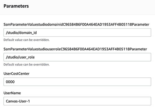
You can also use cost allocation tags that are attached to each user. For example, UserCostCenter is a sample tag where you can add the name of each user.
Key considerations for governing ML environments using Canvas
Now that we have provisioned and deployed an AWS Service Catalog portfolio focused on Canvas, we’d like to highlight a few considerations to govern the Canvas-based ML environments focused on the domain and the user profile.
The following are considerations regarding the Studio domain:
- Networking for Canvas is managed at the Studio domain level, where the domain is deployed on a private VPC subnet for secure connectivity. See Securing Amazon SageMaker Studio connectivity using a private VPC to learn more.
- A default IAM execution role is defined at the domain level. This default role is assigned to all Canvas users in the domain.
- Encryption is done using AWS KMS by encrypting the EFS volume in the domain. For additional controls, you can specify your own managed key, also known as a customer managed key (CMK). See Protect Data at Rest Using Encryption to learn more.
- The ability to upload files from your local disk is done by attaching a cross-origin resource sharing (CORS) policy to the S3 bucket used by Canvas. See Give Your Users Permissions to Upload Local Files to learn more.
The following are considerations regarding the user profile:
- Authentication in Studio can be done both through single sign-on (SSO) and IAM. If you have an existing identity provider to federate users to access the console, you can assign a Studio user profile to each federated identity using IAM. See the section Assigning the policy to Studio users in Configuring Amazon SageMaker Studio for teams and groups with complete resource isolation to learn more.
- You can assign IAM execution roles to each user profile. While using Studio, a user assumes the role mapped to their user profile that overrides the default execution role. You can use this for fine-grained access controls within a team.
- You can achieve isolation using attribute-based access controls (ABAC) to ensure users can only access the resources for their team. See Configuring Amazon SageMaker Studio for teams and groups with complete resource isolation to learn more.
- You can perform fine-grained cost tracking by applying cost allocation tags to user profiles.
Clean up
In order to clean up the resources created by the AWS CDK stack above, navigate over to the AWS CloudFormation stacks page and delete the Canvas stacks. You can also run cdk destroy from within the repository folder, to do the same.
Conclusion
In this post, we shared how you can quickly and easily provision ML environments with Canvas using AWS Service Catalog and the AWS CDK. We discussed how you can create a portfolio on AWS Service Catalog, provision the portfolio, and deploy it in your account. IT administrators can use this method to deploy and manage users, sessions, and associated costs while provisioning Canvas.
Learn more about Canvas on the product page and the Developer Guide. For further reading, you can learn how to enable business analysts to access SageMaker Canvas using AWS SSO without the console. You can also learn how business analysts and data scientists can collaborate faster using Canvas and Studio.
About the Authors
 Davide Gallitelli is a Specialist Solutions Architect for AI/ML in the EMEA region. He is based in Brussels and works closely with customers throughout Benelux. He has been a developer since he was very young, starting to code at the age of 7. He started learning AI/ML at university, and has fallen in love with it since then.
 Sofian Hamiti is an AI/ML specialist Solutions Architect at AWS. He helps customers across industries accelerate their AI/ML journey by helping them build and operationalize end-to-end machine learning solutions.
 Shyam Srinivasan is a Principal Product Manager on the AWS AI/ML team, leading product management for Amazon SageMaker Canvas. Shyam cares about making the world a better place through technology and is passionate about how AI and ML can be a catalyst in this journey.
 Avi Patel works as a software engineer on the Amazon SageMaker Canvas team. His background consists of working full stack with a frontend focus. In his spare time, he likes to contribute to open source projects in the crypto space and learn about new DeFi protocols.
 Jared Heywood is a Senior Business Development Manager at AWS. He is a global AI/ML specialist helping customers with no-code machine learning. He has worked in the AutoML space for the past 5 years and launched products at Amazon like Amazon SageMaker JumpStart and Amazon SageMaker Canvas.
New features for Amazon SageMaker Pipelines and the Amazon SageMaker SDK
Amazon SageMaker Pipelines allows data scientists and machine learning (ML) engineers to automate training workflows, which helps you create a repeatable process to orchestrate model development steps for rapid experimentation and model retraining. You can automate the entire model build workflow, including data preparation, feature engineering, model training, model tuning, and model validation, and catalog it in the model registry. You can configure pipelines to run automatically at regular intervals or when certain events are triggered, or you can run them manually as needed.
In this post, we highlight some of the enhancements to the Amazon SageMaker SDK and introduce new features of Amazon SageMaker Pipelines that make it easier for ML practitioners to build and train ML models.
Pipelines continues to innovate its developer experience, and with these recent releases, you can now use the service in a more customized way:
-
2.99.0, 2.101.1, 2.102.0, 2.104.0 – Updated documentation on
PipelineVariableusage for estimator, processor, tuner, transformer, and model base classes, Amazon models, and framework models. There will be additional changes coming with newer versions of the SDK to support all subclasses of estimators and processors. - 2.90.0 – Availability of ModelStep for integrated model resource creation and registration tasks.
- 2.88.2 – Availability of PipelineSession for managed interaction with SageMaker entities and resources.
- 2.88.2 – Subclass compatibility for workflow pipeline job steps so you can build job abstractions and configure and run processing, training, transform, and tuning jobs as you would without a pipeline.
- 2.76.0 – Availability of FailStep to conditionally stop a pipeline with a failure status.
In this post, we walk you through a workflow using a sample dataset with a focus on model building and deployment to demonstrate how to implement Pipelines’s new features. By the end, you should have enough information to successfully use these newer features and simplify your ML workloads.
Features overview
Pipelines offers the following new features:
-
Pipeline variable annotation – Certain method parameters accept multiple input types, including
PipelineVariables, and additional documentation has been added to clarify wherePipelineVariablesare supported in both the latest stable version of SageMaker SDK documentation and the init signature of the functions. For example, in the following TensorFlow estimator, the init signature now shows thatmodel_dirandimage_urisupportPipelineVariables, whereas the other parameters do not. For more information, refer to TensorFlow Estimator.- Before:
- After:
-
Pipeline session – PipelineSession is a new concept introduced to bring unity across the SageMaker SDK and introduces lazy initialization of the pipeline resources (the run calls are captured but not run until the pipeline is created and run). The
PipelineSessioncontext inherits theSageMakerSessionand implements convenient methods for you to interact with other SageMaker entities and resources, such as training jobs, endpoints, and input datasets stored in Amazon Simple Storage Service (Amazon S3). -
Subclass compatibility with workflow pipeline job steps – You can now build job abstractions and configure and run processing, training, transform, and tuning jobs as you would without a pipeline.
- For example, creating a processing step with
SKLearnProcessorpreviously required the following: - As we see in the preceding code,
ProcessingStepneeds to do basically the same preprocessing logic as.run, just without initiating the API call to start the job. But with subclass compatibility now enabled with workflow pipeline job steps, we declare thestep_argsargument that takes the preprocessing logic with .run so you can build a job abstraction and configure it as you would use it without Pipelines. We also pass in thepipeline_session, which is aPipelineSessionobject, instead ofsagemaker_sessionto make sure the run calls are captured but not called until the pipeline is created and run. See the following code:
- For example, creating a processing step with
-
Model step (a streamlined approach with model creation and registration steps) –Pipelines offers two step types to integrate with SageMaker models:
CreateModelStepandRegisterModel. You can now achieve both using only theModelSteptype. Note that aPipelineSessionis required to achieve this. This brings similarity between the pipeline steps and the SDK.- Before:
-
- After:
-
Fail step (conditional stop of the pipeline run) –
FailStepallows a pipeline to be stopped with a failure status if a condition is met, such as if the model score is below a certain threshold.
Solution overview
In this solution, your entry point is the Amazon SageMaker Studio integrated development environment (IDE) for rapid experimentation. Studio offers an environment to manage the end-to-end Pipelines experience. With Studio, you can bypass the AWS Management Console for your entire workflow management. For more information on managing Pipelines from within Studio, refer to View, Track, and Execute SageMaker Pipelines in SageMaker Studio.
The following diagram illustrates the high-level architecture of the ML workflow with the different steps to train and generate inferences using the new features.

The pipeline includes the following steps:
- Preprocess data to build features required and split data into train, validation, and test datasets.
- Create a training job with the SageMaker XGBoost framework.
- Evaluate the trained model using the test dataset.
- Check if the AUC score is above a predefined threshold.
- If the AUC score is less than the threshold, stop the pipeline run and mark it as failed.
- If the AUC score is greater than the threshold, create a SageMaker model and register it in the SageMaker model registry.
- Apply batch transform on the given dataset using the model created in the previous step.
Prerequisites
To follow along with this post, you need an AWS account with a Studio domain.
Pipelines is integrated directly with SageMaker entities and resources, so you don’t need to interact with any other AWS services. You also don’t need to manage any resources because it’s a fully managed service, which means that it creates and manages resources for you. For more information on the various SageMaker components that are both standalone Python APIs along with integrated components of Studio, see the SageMaker product page.
Before getting started, install SageMaker SDK version >= 2.104.0 and xlrd >=1.0.0 within the Studio notebook using the following code snippet:
ML workflow
For this post, you use the following components:
-
Data preparation
- SageMaker Processing – SageMaker Processing is a fully managed service allowing you to run custom data transformations and feature engineering for ML workloads.
-
Model building
- Studio notebooks – One-click notebooks with elastic compute.
- SageMaker built-in algorithms – XGBoost as a built-in algorithm.
-
Model training and evaluation
- One-click training – The SageMaker distributed training feature. SageMaker provides distributed training libraries for data parallelism and model parallelism. The libraries are optimized for the SageMaker training environment, help adapt your distributed training jobs to SageMaker, and improve training speed and throughput.
- SageMaker Experiments – Experiments is a capability of SageMaker that lets you organize, track, compare, and evaluate your ML iterations.
- SageMaker batch transform – Batch transform or offline scoring is a managed service in SageMaker that lets you predict on a larger dataset using your ML models.
-
Workflow orchestration
- SageMaker Pipelines – ML workflow orchestration and automation
A SageMaker pipeline is a series of interconnected steps defined by a JSON pipeline definition. It encodes a pipeline using a directed acyclic graph (DAG). The DAG gives information on the requirements for and relationships between each step of the pipeline, and its structure is determined by the data dependencies between steps. These dependencies are created when the properties of a step’s output are passed as the input to another step.
The following diagram illustrates the different steps in the SageMaker pipeline (for a churn prediction use case) where the connections between the steps are inferred by SageMaker based on the inputs and outputs defined by the step definitions.
The next sections walk through creating each step of the pipeline and running the entire pipeline once created.

Project structure
Let’s start with the project structure:
-
/sm-pipelines-end-to-end-example – The project name
- /data – The datasets
-
/pipelines – The code files for pipeline components
- /customerchurn
- preprocess.py
- evaluate.py
- /customerchurn
- sagemaker-pipelines-project.ipynb – A notebook walking through the modeling workflow using Pipelines’s new features
Download the dataset
To follow along with this post, you need to download and save the sample dataset under the data folder within the project home directory, which saves the file in Amazon Elastic File System (Amazon EFS) within the Studio environment.
Build the pipeline components
Now you’re ready to build the pipeline components.
Import statements and declare parameters and constants
Create a Studio notebook called sagemaker-pipelines-project.ipynb within the project home directory. Enter the following code block in a cell, and run the cell to set up SageMaker and S3 client objects, create PipelineSession, and set up the S3 bucket location using the default bucket that comes with a SageMaker session:
Pipelines supports parameterization, which allows you to specify input parameters at runtime without changing your pipeline code. You can use the modules available under the sagemaker.workflow.parameters module, such as ParameterInteger, ParameterFloat, and ParameterString, to specify pipeline parameters of various data types. Run the following code to set up multiple input parameters:
Generate a batch dataset
Generate the batch dataset, which you use later in the batch transform step:
Upload data to an S3 bucket
Upload the datasets to Amazon S3:
Define a processing script and processing step
In this step, you prepare a Python script to do feature engineering, one hot encoding, and curate the training, validation, and test splits to be used for model building. Run the following code to build your processing script:
Next, run the following code block to instantiate the processor and the Pipelines step to run the processing script. Because the processing script is written in Pandas, you use a SKLearnProcessor. The Pipelines ProcessingStep function takes the following arguments: the processor, the input S3 locations for raw datasets, and the output S3 locations to save processed datasets.
Define a training step
Set up model training using a SageMaker XGBoost estimator and the Pipelines TrainingStep function:
Define the evaluation script and model evaluation step
Run the following code block to evaluate the model once trained. This script encapsulates the logic to check if the AUC score meets the specified threshold.
Next, run the following code block to instantiate the processor and the Pipelines step to run the evaluation script. Because the evaluation script uses the XGBoost package, you use a ScriptProcessor along with the XGBoost image. The Pipelines ProcessingStep function takes the following arguments: the processor, the input S3 locations for raw datasets, and the output S3 locations to save processed datasets.
Define a create model step
Run the following code block to create a SageMaker model using the Pipelines model step. This step utilizes the output of the training step to package the model for deployment. Note that the value for the instance type argument is passed using the Pipelines parameter you defined earlier in the post.
Define a batch transform step
Run the following code block to run batch transformation using the trained model with the batch input created in the first step:
Define a register model step
The following code registers the model within the SageMaker model registry using the Pipelines model step:
Define a fail step to stop the pipeline
The following code defines the Pipelines fail step to stop the pipeline run with an error message if the AUC score doesn’t meet the defined threshold:
Define a condition step to check AUC score
The following code defines a condition step to check the AUC score and conditionally create a model and run a batch transformation and register a model in the model registry, or stop the pipeline run in a failed state:
Build and run the pipeline
After defining all of the component steps, you can assemble them into a Pipelines object. You don’t need to specify the order of pipeline because Pipelines automatically infers the order sequence based on the dependencies between the steps.
Run the following code in a cell in your notebook. If the pipeline already exists, the code updates the pipeline. If the pipeline doesn’t exist, it creates a new one.
Conclusion
In this post, we introduced some of the new features now available with Pipelines along with other built-in SageMaker features and the XGBoost algorithm to develop, iterate, and deploy a model for churn prediction. The solution can be extended with additional data sources
to implement your own ML workflow. For more details on the steps available in the Pipelines workflow, refer to Amazon SageMaker Model Building Pipeline and SageMaker Workflows. The AWS SageMaker Examples GitHub repo has more examples around various use cases using Pipelines.
About the Authors
 Jerry Peng is a software development engineer with AWS SageMaker. He focuses on building end-to-end large-scale MLOps system from training to model monitoring in production. He is also passionate about bringing the concept of MLOps to broader audience.
 Dewen Qi is a Software Development Engineer in AWS. She currently focuses on developing and improving SageMaker Pipelines. Outside of work, she enjoys practicing Cello.
 Gayatri Ghanakota is a Sr. Machine Learning Engineer with AWS Professional Services. She is passionate about developing, deploying, and explaining AI/ ML solutions across various domains. Prior to this role, she led multiple initiatives as a data scientist and ML engineer with top global firms in the financial and retail space. She holds a master’s degree in Computer Science specialized in Data Science from the University of Colorado, Boulder.
 Rupinder Grewal is a Sr Ai/ML Specialist Solutions Architect with AWS. He currently focuses on serving of models and MLOps on SageMaker. Prior to this role he has worked as Machine Learning Engineer building and hosting models. Outside of work he enjoys playing tennis and biking on mountain trails.
 Ray Li is a Sr. Data Scientist with AWS Professional Services. His specialty focuses on building and operationalizing AI/ML solutions for customers of varying sizes, ranging from startups to enterprise organizations. Outside of work, Ray enjoys fitness and traveling.

Quantization for Fast and Environmentally Sustainable Reinforcement Learning
Deep reinforcement learning (RL) continues to make great strides in solving real-world sequential decision-making problems such as balloon navigation, nuclear physics, robotics, and games. Despite its promise, one of its limiting factors is long training times. While the current approach to speed up RL training on complex and difficult tasks leverages distributed training scaling up to hundreds or even thousands of computing nodes, it still requires the use of significant hardware resources which makes RL training expensive, while increasing its environmental impact. However, recent work [1, 2] indicates that performance optimizations on existing hardware can reduce the carbon footprint (i.e., total greenhouse gas emissions) of training and inference.
RL can also benefit from similar system optimization techniques that can reduce training time, improve hardware utilization and reduce carbon dioxide (CO2) emissions. One such technique is quantization, a process that converts full-precision floating point (FP32) numbers to lower precision (int8) numbers and then performs computation using the lower precision numbers. Quantization can save memory storage cost and bandwidth for faster and more energy-efficient computation. Quantization has been successfully applied to supervised learning to enable edge deployments of machine learning (ML) models and achieve faster training. However, there remains an opportunity to apply quantization to RL training.
To that end, we present “QuaRL: Quantization for Fast and Environmentally SustainableReinforcement Learning”, published in the Transactions of Machine Learning Research journal, which introduces a new paradigm called ActorQ that applies quantization to speed up RL training by 1.5-5.4x while maintaining performance. Additionally, we demonstrate that compared to training in full-precision, the carbon footprint is also significantly reduced by a factor of 1.9-3.8x.
Applying Quantization to RL Training
In traditional RL training, a learner policy is applied to an actor, which uses the policy to explore the environment and collect data samples. The samples collected by the actor are then used by the learner to continuously refine the initial policy. Periodically, the policy trained on the learner side is used to update the actor’s policy. To apply quantization to RL training, we develop the ActorQ paradigm. ActorQ performs the same sequence described above, with one key difference being that the policy update from learner to actors is quantized, and the actor explores the environment using the int8 quantized policy to collect samples.
Applying quantization to RL training in this fashion has two key benefits. First, it reduces the memory footprint of the policy. For the same peak bandwidth, less data is transferred between learners and actors, which reduces the communication cost for policy updates from learners to actors. Second, the actors perform inference on the quantized policy to generate actions for a given environment state. The quantized inference process is much faster when compared to performing inference in full precision.
 |
| An overview of traditional RL training (left) and ActorQ RL training (right). |
In ActorQ, we use the ACME distributed RL framework. The quantizer block performs uniform quantization that converts the FP32 policy to int8. The actor performs inference using optimized int8 computations. Though we use uniform quantization when designing the quantizer block, we believe that other quantization techniques can replace uniform quantization and produce similar results. The samples collected by the actors are used by the learner to train a neural network policy. Periodically the learned policy is quantized by the quantizer block and broadcasted to the actors.
Quantization Improves RL Training Time and Performance
We evaluate ActorQ in a range of environments, including the Deepmind Control Suite and the OpenAI Gym. We demonstrate the speed-up and improved performance of D4PG and DQN. We chose D4PG as it was the best learning algorithm in ACME for Deepmind Control Suite tasks, and DQN is a widely used and standard RL algorithm.
We observe a significant speedup (between 1.5x and 5.41x) in training RL policies. More importantly, performance is maintained even when actors perform int8 quantized inference. The figures below demonstrate this for the D4PG and DQN agents for Deepmind Control Suite and OpenAI Gym tasks.
 |
| A comparison of RL training using the FP32 policy (q=32) and the quantized int8 policy (q=8) for D4PG agents on various Deepmind Control Suite tasks. Quantization achieves speed-ups of 1.5x to 3.06x. |
 |
| A comparison of RL training using the FP32 policy (q=32) and the quantized int8 policy (q=8) for DQN agents in the OpenAI Gym environment. Quantization achieves a speed-up of 2.2x to 5.41x. |
Quantization Reduces Carbon Emission
Applying quantization in RL using ActorQ improves training time without affecting performance. The direct consequence of using the hardware more efficiently is a smaller carbon footprint. We measure the carbon footprint improvement by taking the ratio of carbon emission when using the FP32 policy during training over the carbon emission when using the int8 policy during training.
In order to measure the carbon emission for the RL training experiment, we use the experiment-impact-tracker proposed in prior work. We instrument the ActorQ system with carbon monitor APIs to measure the energy and carbon emissions for each training experiment.
Compared to the carbon emission when running in full precision (FP32), we observe that the quantization of policies reduces the carbon emissions anywhere from 1.9x to 3.76x, depending on the task. As RL systems are scaled to run on thousands of distributed hardware cores and accelerators, we believe that the absolute carbon reduction (measured in kilograms of CO2) can be quite significant.
 |
| Carbon emission comparison between training using a FP32 policy and an int8 policy. The X-axis scale is normalized to the carbon emissions of the FP32 policy. Shown by the red bars greater than 1, ActorQ reduces carbon emissions. |
Conclusion and Future Directions
We introduce ActorQ, a novel paradigm that applies quantization to RL training and achieves speed-up improvements of 1.5-5.4x while maintaining performance. Additionally, we demonstrate that ActorQ can reduce RL training’s carbon footprint by a factor of 1.9-3.8x compared to training in full-precision without quantization.
ActorQ demonstrates that quantization can be effectively applied to many aspects of RL, from obtaining high-quality and efficient quantized policies to reducing training times and carbon emissions. As RL continues to make great strides in solving real-world problems, we believe that making RL training sustainable will be critical for adoption. As we scale RL training to thousands of cores and GPUs, even a 50% improvement (as we have experimentally demonstrated) will generate significant savings in absolute dollar cost, energy, and carbon emissions. Our work is the first step toward applying quantization to RL training to achieve efficient and environmentally sustainable training.
While our design of the quantizer in ActorQ relied on simple uniform quantization, we believe that other forms of quantization, compression and sparsity can be applied (e.g., distillation, sparsification, etc.). We hope that future work will consider applying more aggressive quantization and compression methods, which may yield additional benefits to the performance and accuracy tradeoff obtained by the trained RL policies.
Acknowledgments
We would like to thank our co-authors Max Lam, Sharad Chitlangia, Zishen Wan, and Vijay Janapa Reddi (Harvard University), and Gabriel Barth-Maron (DeepMind), for their contribution to this work. We also thank the Google Cloud team for providing research credits to seed this work.