This paper was accepted at the workshop “Causality for Real-world Impact” at NeurIPS 2022.
The Apple Watch encourages users to stand throughout the day by delivering a notification onto the users’ wrist if they have been sitting for the first 50 minutes of an hour. This simple behavioral intervention exemplifies the classical definition of nudge as a choice architecture that alters behavior without forbidding options or significantly changing economic incentives. In order to estimate from observational data the causal effect of the notification on the user’s standing probability through-out…Apple Machine Learning Research
Improving Generalization with Physical Equations
This paper was accepted at the workshop “Machine Learning 4 Physical Sciences” at NeurIPS 2022.
Hybrid modelling reduces the misspecification of expert physical models with a machine learning (ML) component learned from data. Similarly to many ML algorithms, hybrid model performance guarantees are limited to the training distribution. To address this limitation, here we introduce a hybrid data augmentation strategy, termed expert augmentation. Based on a probabilistic formalization of hybrid modelling, we demonstrate that expert augmentation improves generalization. We validate the practical…Apple Machine Learning Research
Multi-layered Mapping of Brain Tissue via Segmentation Guided Contrastive Learning
Mapping the wiring and firing activity of the human brain is fundamental to deciphering how we think — how we sense the world, learn, decide, remember, and create — as well as what issues can arise in brain disease or dysfunction. Recent efforts have delivered publicly available brain maps (high-resolution 3D mapping of brain cells and their connectivities) at unprecedented quality and scale, such as H01, a 1.4 petabyte nanometer-scale digital reconstruction of a sample of human brain tissue from Harvard / Google, and the cubic millimeter mouse cortex dataset from our colleagues at the MICrONS consortium.
To interpret brain maps at this scale requires multiple layers of analysis, including the identification of synaptic connections, cellular subcompartments, and cell types. Machine learning and computer vision technology have played a central role in enabling these analyses, but deploying such systems is still a laborious process, requiring hours of manual ground truth labeling by expert annotators and significant computational resources. Moreover, some important tasks, such as identifying the cell type from only a small fragment of axon or dendrite, can be challenging even for human experts, and have not yet been effectively automated.
Today, in “Multi-Layered Maps of Neuropil with Segmentation-Guided Contrastive Learning”, we are announcing Segmentation-Guided Contrastive Learning of Representations (SegCLR), a method for training rich, generic representations of cellular morphology (the cell’s shape) and ultrastructure (the cell’s internal structure) without laborious manual effort. SegCLR produces compact vector representations (i.e., embeddings) that are applicable across diverse downstream tasks (e.g., local classification of cellular subcompartments, unsupervised clustering), and are even able to identify cell types from only small fragments of a cell. We trained SegCLR on both the H01 human cortex dataset and the MICrONS mouse cortex dataset, and we are releasing the resulting embedding vectors, about 8 billion in total, for researchers to explore.
| From brain cells segmented out of a 3D block of tissue, SegCLR embeddings capture cellular morphology and ultrastructure and can be used to distinguish cellular subcompartments (e.g., dendritic spine versus dendrite shaft) or cell types (e.g., pyramidal versus microglia cell). |
Representing Cellular Morphology and Ultrastructure
SegCLR builds on recent advances in self-supervised contrastive learning. We use a standard deep network architecture to encode inputs comprising local 3D blocks of electron microscopy data (about 4 micrometers on a side) into 64-dimensional embedding vectors. The network is trained via a contrastive loss to map semantically related inputs to similar coordinates in the embedding space. This is close to the popular SimCLR setup, except that we also require an instance segmentation of the volume (tracing out individual cells and cell fragments), which we use in two important ways.
First, the input 3D electron microscopy data are explicitly masked by the segmentation, forcing the network to focus only on the central cell within each block. Second, we leverage the segmentation to automatically define which inputs are semantically related: positive pairs for the contrastive loss are drawn from nearby locations on the same segmented cell and trained to have similar representations, while inputs drawn from different cells are trained to have dissimilar representations. Importantly, publicly available automated segmentations of the human and mouse datasets were sufficiently accurate to train SegCLR without requiring laborious review and correction by human experts.
 |
| SegCLR is trained to represent rich cellular features without manual labeling. Top: The SegCLR architecture maps local masked 3D views of electron microscopy data to embedding vectors. Only the microscopy volume and a draft automated instance segmentation are required. Bottom: The segmentation is also used to define positive versus negative example pairs, whose representations are pushed closer together (positives, blue arrows) or further apart (negatives, red arrows) during training. |
Reducing Annotation Training Requirements by Three Orders of Magnitude
SegCLR embeddings can be used in diverse downstream settings, whether supervised (e.g., training classifiers) or unsupervised (e.g., clustering or content-based image retrieval). In the supervised setting, embeddings simplify the training of classifiers, and can greatly reduce ground truth labeling requirements. For example, we found that for identifying cellular subcompartments (axon, dendrite, soma, etc.) a simple linear classifier trained on top of SegCLR embeddings outperformed a fully supervised deep network trained on the same task, while using only about one thousand labeled examples instead of millions.
 |
| We assessed the classification performance for axon, dendrite, soma, and astrocyte subcompartments in the human cortex dataset via mean F1-Score, while varying the number of training examples used. Linear classifiers trained on top of SegCLR embeddings matched or exceeded the performance of a fully supervised deep classifier (horizontal line), while using a fraction of the training data. |
Distinguishing Cell Types, Even from Small Fragments
Distinguishing different cell types is an important step towards understanding how brain circuits develop and function in health and disease. Human experts can learn to identify some cortical cell types based on morphological features, but manual cell typing is laborious and ambiguous cases are common. Cell typing also becomes more difficult when only small fragments of cells are available, which is common for many cells in current connectomic reconstructions.
 |
| Human experts manually labeled cell types for a small number of proofread cells in each dataset. In the mouse cortex dataset, experts labeled six neuron types (top) and four glia types (not shown). In the human cortex dataset, experts labeled two neuron types (not shown) and four glia types (bottom). (Rows not to scale with each other.) |
We found that SegCLR accurately infers human and mouse cell types, even for small fragments. Prior to classification, we collected and averaged embeddings within each cell over a set aggregation distance, defined as the radius from a central point. We found that human cortical cell types can be identified with high accuracy for aggregation radii as small as 10 micrometers, even for types that experts find difficult to distinguish, such as microglia (MGC) versus oligodendrocyte precursor cells (OPC).
 |
| SegCLR can classify cell types, even from small fragments. Left: Classification performance over six human cortex cell types for shallow ResNet models trained on SegCLR embeddings for different sized cell fragments. Aggregation radius zero corresponds to very small fragments with only a single embedding. Cell type performance reaches high accuracy (0.938 mean F1-Score) for fragments with aggregation radii of only 10 micrometers (boxed point). Right: Class-wise confusion matrix at 10 micrometers aggregation radius. Darker shading along the diagonal indicates that predicted cell types agree with expert labels in most cases. AC: astrocyte; MGC: microglia cell; OGC: oligodendrocyte cell; OPC: oligodendrocyte precursor cell; E: excitatory neuron; I: inhibitory neuron. |
In the mouse cortex, ten cell types could be distinguished with high accuracy at aggregation radii of 25 micrometers.
 |
| Left: Classification performance over the ten mouse cortex cell types reaches 0.832 mean F1-Score for fragments with aggregation radius 25 micrometers (boxed point). Right: The class-wise confusion matrix at 25 micrometers aggregation radius. Boxes indicate broad groups (glia, excitatory neurons, and inhibitory interneurons). P: pyramidal cell; THLC: thalamocortical axon; BC: basket cell; BPC: bipolar cell; MC: Martinotti cell; NGC: neurogliaform cell. |
In additional cell type applications, we used unsupervised clustering of SegCLR embeddings to reveal further neuronal subtypes, and demonstrated how uncertainty estimation can be used to restrict classification to high confidence subsets of the dataset, e.g., when only a few cell types have expert labels.
Revealing Patterns of Brain Connectivity
Finally, we showed how SegCLR can be used for automated analysis of brain connectivity by cell typing the synaptic partners of reconstructed cells throughout the mouse cortex dataset. Knowing the connectivity patterns between specific cell types is fundamental to interpreting large-scale connectomic reconstructions of brain wiring, but this typically requires manual tracing to identify partner cell types. Using SegCLR, we replicated brain connectivity findings that previously relied on intensive manual tracing, while extending their scale in terms of the number of synapses, cell types, and brain areas analyzed. (See the paper for further details.)
 |
| SegCLR automated analysis of brain connectivity. Top: An example mouse pyramidal cell, with synapse locations color-coded according to whether the synaptic partner was classified as inhibitory (blue), excitatory (red), or unknown (black). Inset shows higher detail of the soma and proximal dendrites. Bottom: We counted how many upstream synaptic partners were classified as thalamocortical axons, which bring input from sensory systems to the cortex. We found that thalamic input arrives primarily at cortical layer L4, the canonical cortical input layer, and preferentially targets primary visual area V1, rather than higher visual areas (HVA). |
What’s Next?
SegCLR captures rich cellular features and can greatly simplify downstream analyses compared to working directly with raw image and segmentation data. We are excited to see what the community can discover using the ~8 billion embeddings we are releasing for the human and mouse cortical datasets (example access code; browsable human and mouse views in Neuroglancer). By reducing complex microscopy data to rich and compact embedding representations, SegCLR opens many novel avenues for biological insight, and may serve as a link to complementary modalities for high-dimensional characterization at the cellular and subcellular levels, such as spatially-resolved transcriptomics.

What Is Denoising?
Anyone who’s taken a photo with a digital camera is likely familiar with a “noisy” image: discolored spots that make the photo lose clarity and sharpness.
Many photographers have tips and tricks to reduce noise in images, including fixing the settings on the camera lens or taking photos in different lighting. But it isn’t just photographs that can look discolored — noise is common in computer graphics, too.
Noise refers to the random variations of brightness and color that aren’t part of the original image. Removing noise from imagery — which is becoming more common in the field of image processing and computer vision — is known as denoising.
Image denoising uses advanced algorithms to remove noise from graphics and renders, making a huge difference to the quality of images. Photorealistic visuals and immersive renders could not be possible without denoising technology.
What Is Denoising?
In computer graphics, images can be made up of both useful information and noise. The latter reduces clarity. The ideal end product of denoising would be a crisp image that only preserves the useful information. When denoising an image, it’s also important to keep visual details and components such as edges, corners, textures and other sharp structures.
To reduce noise without affecting the visual details, three types of signals in an image must be targeted by denoising:
- Diffuse — scattered lighting reflected in all directions;
- Specular or reflections — lighting reflected in a particular direction; and
- Infinite light-source shadows — sunlight, shadows and any other visible light source.
To create the clearest image, a user must cast thousands of rays in directions following the diffuse and specular signals. Often in real-time ray tracing, however, only one ray per pixel or even less is used.
Denoising is necessary in real-time ray tracing because of the relatively low ray counts to maintain interactive performance.

How Does Denoising Work?
Image denoising is commonly based on three techniques: spatial filtering, temporal accumulation, and machine learning and deep learning reconstruction.

Spatial filtering selectively alters parts of an image by reusing similar neighboring pixels. The advantage of spatial filtering is that it doesn’t produce temporal lag, which is the inability to immediately respond to changing flow conditions. However, spatial filtering introduces blurriness and muddiness, as well as temporal instability, which refers to flickering and visual imperfections in the image.
Temporal accumulation reuses data from the previous frame to determine if there are any artifacts — or visual anomalies — in the current frame that can be corrected. Although temporal accumulation introduces temporal lag, it doesn’t produce blurriness. Instead, it adds temporal stability to reduce flickering and artifacts over multiple frames.

Machine learning and deep learning reconstruction uses a neural network to reconstruct the signal. The neural network is trained using various noisy and reference signals. Though the reconstructed signal for a single frame can look complete, it can become temporally unstable over time, so a form of temporal stabilization is needed.
Denoising in Images
Denoising provides users with immediate visual feedback, so they can see and interact with graphics and designs. This allows them to experiment with variables like light, materials, viewing angle and shadows.
Solutions like NVIDIA Real-Time Denoisers (NRD) make denoising techniques more accessible for developers to integrate into pipelines. NRD is a spatio-temporal denoising library that’s agnostic to application programming interfaces and designed to work with low rays per pixel.
NRD uses input signals and environmental conditions to deliver results comparable to ground-truth images. See NRD in action below:
With NRD, developers can achieve real-time results using a limited budget of rays per pixel. In the video above, viewers can see the heavy lifting that NRD does in real time to resolve image noise.
Popular games such as Dying Light 2 and Hitman III use NRD for denoising.

NRD supports the denoising of diffuse, specular or reflections, and shadow signals. The denoisers included in NRD are:
- ReBLUR — based on the idea of self-stabilizing, recurrent blurring. It’s designed to work with diffuse and specular signals generated with low ray budgets.
- SIGMA — a fast shadow denoiser. It supports shadows from any type of light source, like the sun and local lights.
- ReLAX — preserves lighting details produced by NVIDIA RTX Direct Illumination, a framework that enables developers to render scenes with millions of dynamic area lights in real time. ReLAX also yields better temporal stability and remains responsive to changing lighting conditions.
See NRD in action with Hitman 3:
Learn about more technologies in game development.
The post What Is Denoising? appeared first on NVIDIA Blog.

NVIDIA AI Turbocharges Industrial Research, Scientific Discovery in the Cloud on Rescale HPC-as-a-Service Platform
Just like many businesses, the world of industrial scientific computing has a data problem.
Solving seemingly intractable challenges — from developing new energy sources and creating new modes of transportation, to addressing mission-critical issues such as driving operational efficiencies and improving customer support — requires massive amounts of high performance computing.
Instead of having to architect, engineer and build ever-more supercomputers, companies such as Electrolux, Denso, Samsung and Virgin Orbit are embracing benefits offered by Rescale’s cloud platform. This makes it possible to scale their accelerated computing in an energy-efficient way and to speed their innovation.
Addressing the industrial scientific community’s rising demand for AI in the cloud, NVIDIA founder and CEO Jensen Huang joined Rescale founder and CEO Joris Poort at the Rescale Big Compute virtual conference, where they announced that Rescale is adopting the NVIDIA AI software portfolio.
NVIDIA AI will bring new capabilities to Rescale’s HPC-as-a-service offerings, which include simulation and engineering software used by hundreds of customers across industries. NVIDIA is also accelerating the Rescale Compute Recommendation Engine announced today, which enables customers to identify the right infrastructure options to optimize cost and speed objectives.
“Fusing principled and data-driven methods, physics-ML AI models let us explore our design space at speeds and scales many orders of magnitude greater than ever before,” Huang said. “Rescale is at the intersection of these major trends. NVIDIA’s accelerated and AI computing platform perfectly complements Rescale to advance industrial scientific computing.”
“Engineers and scientists working on breakthrough innovations need integrated cloud platforms that put R&D software and accelerated computing at their fingertips,” said Poort. “We’ve helped customers speed discoveries and save costs with NVIDIA-accelerated HPC, and adding NVIDIA AI Enterprise to the Rescale platform will bring together the most advanced computing capabilities with the best of AI, and support an even broader range of AI-powered workflows R&D leaders can run on any cloud of their choice.”
Expanding HPC to New Horizons in the Cloud With NVIDIA AI
The companies announced that they are working to bring NVIDIA AI Enterprise to Rescale, broadening the cloud platform’s offerings to include NVIDIA-supported AI workflows and processing engines. Once it’s available, customers will be able to develop AI applications in any leading cloud, with support from NVIDIA.
The globally adopted software of the NVIDIA AI platform, NVIDIA AI Enterprise includes essential processing engines for each step of the AI workflow, from data processing and AI model training to simulation and large-scale deployment.
NVIDIA AI enables organizations to develop predictive models to complement and expand industrial HPC research and development with applications such as computer vision, route and supply chain optimization, robotics simulations and more.
The Rescale software catalog provides access to hundreds of NVIDIA-accelerated containerized applications and pretrained AI models on NVIDIA NGC, and allows customers to run simulations on demand and scale up or down as needed.
NVIDIA Modulus to Speed Physics-Based Machine Learning
Rescale now offers the NVIDIA Modulus framework for developing physics machine learning neural network models to support a broad range of engineering use cases.
Modulus blends the power of physics with data to build high-fidelity models that enable near-real-time simulations. With just a few clicks on the Rescale platform, Modulus will allow customers to run their entire AI-driven simulation workflow, from data pre-processing and model training to inference and model deployment.
On-Prem to Cloud Workflow Orchestration Expands Flexibility
Rescale is additionally integrating the NVIDIA Base Command Platform AI developer workflow management software, which can orchestrate workloads across clouds to on-premises NVIDIA DGX systems.
Rescale’s HPC-as-a-service platform is accelerated by NVIDIA on leading cloud service provider platforms, including Amazon Web Services, Google Cloud, Microsoft Azure and Oracle Cloud Infrastructure. Rescale is a member of the NVIDIA Inception program.
To learn more, watch Huang and Poort discuss the news in the replay of the Big Compute keynote address.
The post NVIDIA AI Turbocharges Industrial Research, Scientific Discovery in the Cloud on Rescale HPC-as-a-Service Platform appeared first on NVIDIA Blog.
How scarce computing shaped Carlos Huertas’s career
At Amazon, he develops machine learning models to help keeping Amazon stores safe and trustworthy for customers and selling partners.Read More
NVIDIA Hopper, Ampere GPUs Sweep Benchmarks in AI Training
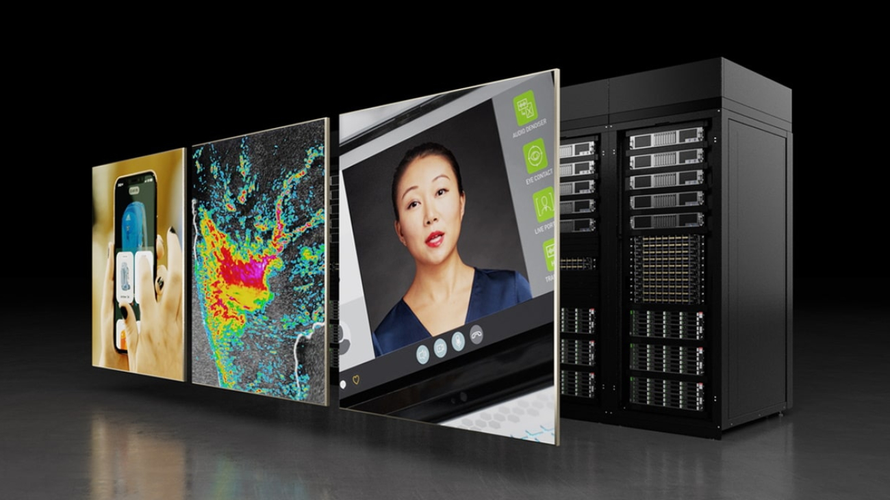
Two months after their debut sweeping MLPerf inference benchmarks, NVIDIA H100 Tensor Core GPUs set world records across enterprise AI workloads in the industry group’s latest tests of AI training.
Together, the results show H100 is the best choice for users who demand utmost performance when creating and deploying advanced AI models.
MLPerf is the industry standard for measuring AI performance. It’s backed by a broad group that includes Amazon, Arm, Baidu, Google, Harvard University, Intel, Meta, Microsoft, Stanford University and the University of Toronto.
In a related MLPerf benchmark also released today, NVIDIA A100 Tensor Core GPUs raised the bar they set last year in high performance computing (HPC).
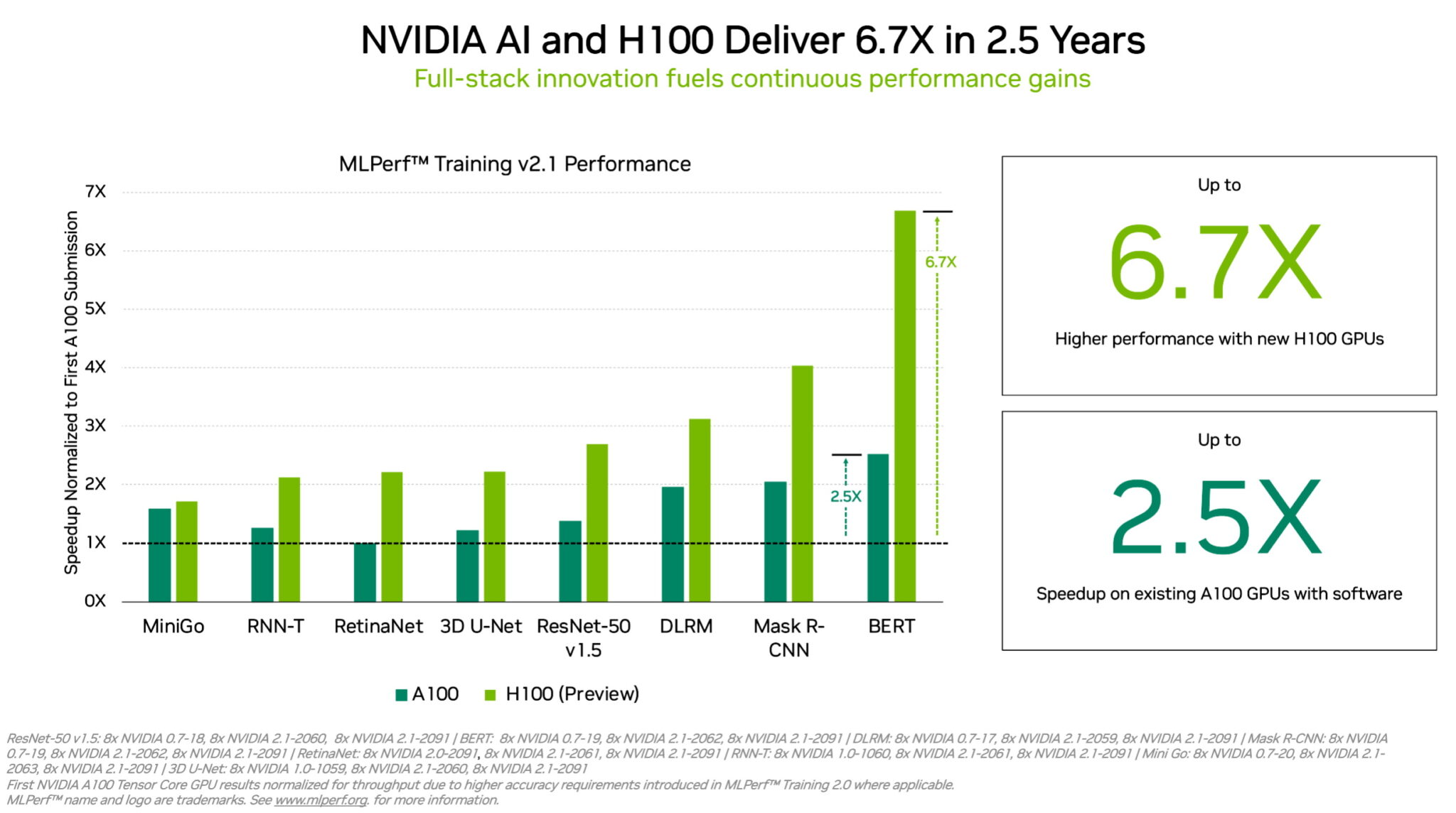
H100 GPUs (aka Hopper) raised the bar in per-accelerator performance in MLPerf Training. They delivered up to 6.7x more performance than previous-generation GPUs when they were first submitted on MLPerf training. By the same comparison, today’s A100 GPUs pack 2.5x more muscle, thanks to advances in software.
Due in part to its Transformer Engine, Hopper excelled in training the popular BERT model for natural language processing. It’s among the largest and most performance-hungry of the MLPerf AI models.
MLPerf gives users the confidence to make informed buying decisions because the benchmarks cover today’s most popular AI workloads — computer vision, natural language processing, recommendation systems, reinforcement learning and more. The tests are peer reviewed, so users can rely on their results.
A100 GPUs Hit New Peak in HPC
In the separate suite of MLPerf HPC benchmarks, A100 GPUs swept all tests of training AI models in demanding scientific workloads run on supercomputers. The results show the NVIDIA AI platform’s ability to scale to the world’s toughest technical challenges.
For example, A100 GPUs trained AI models in the CosmoFlow test for astrophysics 9x faster than the best results two years ago in the first round of MLPerf HPC. In that same workload, the A100 also delivered up to a whopping 66x more throughput per chip than an alternative offering.
The HPC benchmarks train models for work in astrophysics, weather forecasting and molecular dynamics. They are among many technical fields, like drug discovery, adopting AI to advance science.
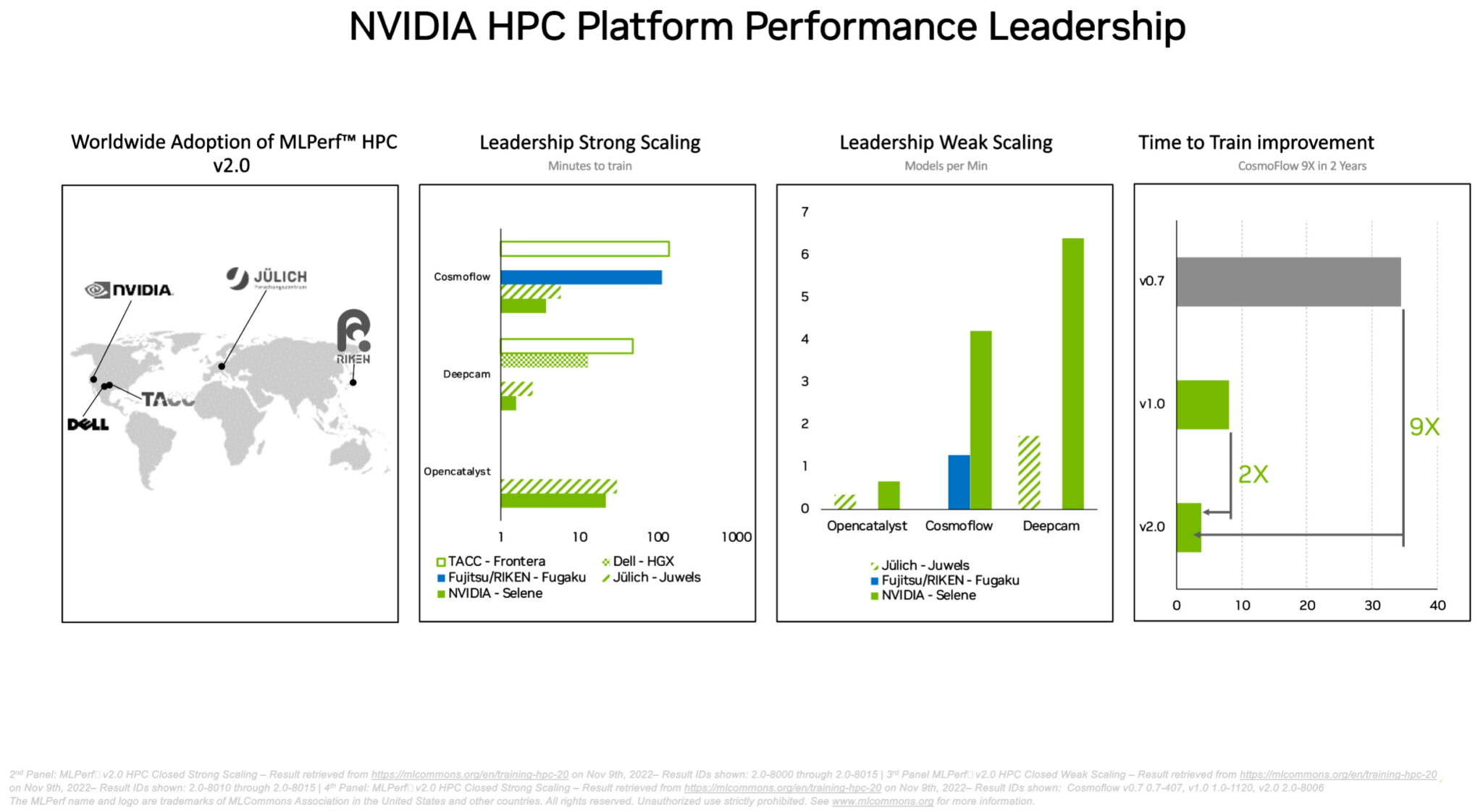
Supercomputer centers in Asia, Europe and the U.S. participated in the latest round of the MLPerf HPC tests. In its debut on the DeepCAM benchmarks, Dell Technologies showed strong results using NVIDIA A100 GPUs.
An Unparalleled Ecosystem
In the enterprise AI training benchmarks, a total of 11 companies, including the Microsoft Azure cloud service, made submissions using NVIDIA A100, A30 and A40 GPUs. System makers including ASUS, Dell Technologies, Fujitsu, GIGABYTE, Hewlett Packard Enterprise, Lenovo and Supermicro used a total of nine NVIDIA-Certified Systems for their submissions.
In the latest round, at least three companies joined NVIDIA in submitting results on all eight MLPerf training workloads. That versatility is important because real-world applications often require a suite of diverse AI models.
NVIDIA partners participate in MLPerf because they know it’s a valuable tool for customers evaluating AI platforms and vendors.
Under the Hood
The NVIDIA AI platform provides a full stack from chips to systems, software and services. That enables continuous performance improvements over time.
For example, submissions in the latest HPC tests applied a suite of software optimizations and techniques described in a technical article. Together they slashed runtime on one benchmark by 5x, to just 22 minutes from 101 minutes.
A second article describes how NVIDIA optimized its platform for the enterprise AI benchmarks. For example, we used NVIDIA DALI to efficiently load and pre-process data for a computer vision benchmark.
All the software used in the tests is available from the MLPerf repository, so anyone can get these world-class results. NVIDIA continuously folds these optimizations into containers available on NGC, a software hub for GPU applications.
The post NVIDIA Hopper, Ampere GPUs Sweep Benchmarks in AI Training appeared first on NVIDIA Blog.
Elastic Weight Consolidation Improves the Robustness of Self-Supervised Learning Methods under Transfer
This paper was accepted at the workshop “Self-Supervised Learning – Theory and Practice” at NeurIPS 2022.
Self-supervised representation learning (SSL) methods provide an effective label-free initial condition for fine-tuning downstream tasks. However, in numerous realistic scenarios, the downstream task might be biased with respect to the target label distribution. This in turn moves the learned fine-tuned model posterior away from the initial (label) bias-free self-supervised model posterior. In this work, we re-interpret SSL fine-tuning under the lens of Bayesian continual learning and…Apple Machine Learning Research
Brain tumor segmentation at scale using AWS Inferentia
Medical imaging is an important tool for the diagnosis and localization of disease. Over the past decade, collections of medical images have grown rapidly, and open repositories such as The Cancer Imaging Archive and Imaging Data Commons have democratized access to this vast imaging data. Computational tools such as machine learning (ML) and artificial intelligence (AI) have emerged as an effective and viable option for rapid analysis of this imaging data. Many algorithms have been developed for different kinds of image analysis. These include classification, segmentation, and localization, to name a few. However, the development of the algorithm and training of the required ML model is only one piece of the larger ML/AI puzzle.
Cost-efficient and high-performance deployment of the model is also vital. Additionally, for a model to be of any use at scale, it must be deployed for inference in a reliable, scalable environment.
In this post, we discuss one possible approach of using native AWS technologies to deploy ML algorithms at scale for a medical imaging use case. We talk about segmenting a tumor from MRI brain scans and cover solution architecture, compute infrastructure, and results.
Solution overview
The solution proposed in this post is based around a trained U-net model using the popular Keras framework and with a sample dataset from the popular Kaggle competition platform.
The trained U-net model is then processed via the AWS Neuron SDK so that it can be optimized to target Amazon EC2 Inf1 instances, featuring AWS Inferentia, the first AWS ML accelerator optimized for inference.
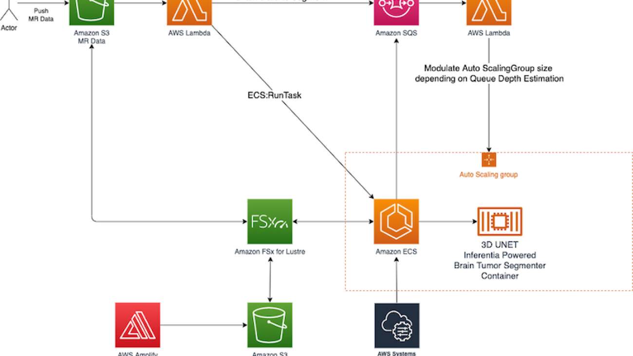
The solution uses a managed elastic architecture with fast storage to ensure that high throughput is maintained across each layer of the solution. The following diagram describes the overall architecture.
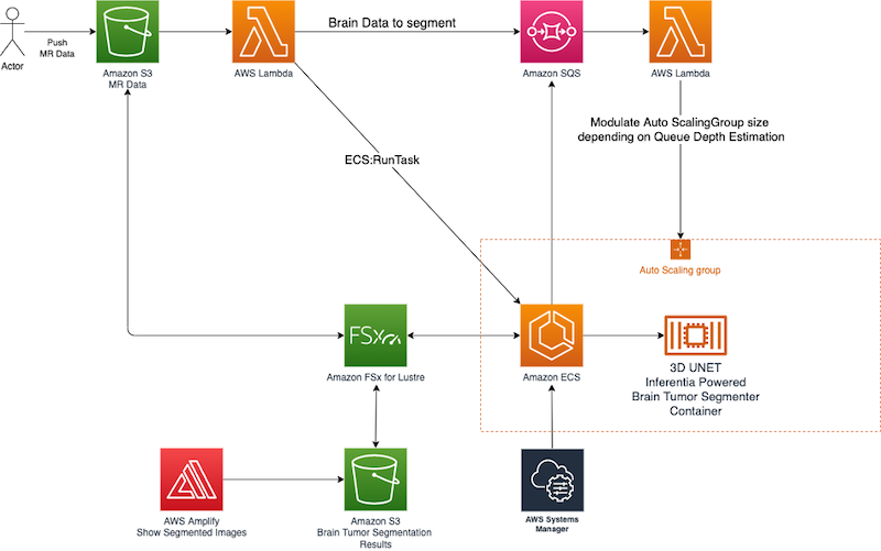
The central idea around the proposed architecture spins around an elastic cluster of AWS Inferentia-powered containers running on Amazon Elastic Container Service (Amazon ECS) serving a U-net model optimized via the AWS Neuron SDK.
The inference nodes: AWS Inferentia

AWS offers various ways to deploy a deep learning model in the cloud. One option uses AWS Inferentia, which is a high-performance ML inference chip designed by AWS.
AWS Inferentia delivers up to 80% lower cost per inference and up to 2.3 times higher throughput than comparable current generation GPU-based Amazon Elastic Compute Cloud (Amazon EC2) instances. With Inf1 instances, you can run high-scale ML inference applications for a variety of medical imaging uses cases. The AWS Neuron SDK optimizes models for deployment onto AWS Inferentia-powered instances.
AWS Neuron consists of a compiler, runtime, and profiling tools that help optimize the performance of workloads for AWS Inferentia.
With AWS Neuron, developers can deploy neural network models using popular frameworks like PyTorch or TensorFlow on AWS Inferentia-based EC2 Inf1 instances.
The workflow to deploy a trained deep learning model into an AWS Inferentia accelerated inference node consists of the following steps:
- Train a neural network model.
- Process the trained model via the AWS Neuron compiler to generate an AWS Inferentia-optimized trained neural model.
- Use the AWS Neuron runtime to load the AWS Inferentia-optimized model to EC2 Inf1 instances and run inference requests.
Inference at scale: An elastic architecture for AWS Inferentia
The architecture elasticity is determined by an AWS Lambda function and Amazon Simple Queue Service (Amazon SQS) queue that receives requests for segmentations initiated by simply uploading the volume that needs to be segmented into an Amazon Simple Storage Service (Amazon S3) bucket.
The AWS Inferentia ECS cluster gets fed from a highly performant Amazon FSx for Lustre file system, which accelerates compute workloads with shared storage that provides sub-millisecond latencies, up to hundreds of GBs/s of throughput, and millions of IOPS.
The following diagram outlines the architecture that enables the AWS Inferentia cluster to be elastic and scale dynamically according the number of inference requests submitted to the whole system.
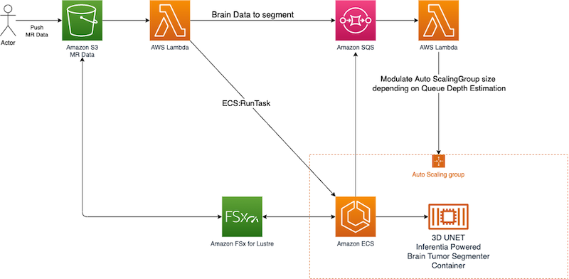
In this architecture, an actor pushes an image volume to an S3 bucket. After the image volume is uploaded to THE S3 bucket, a Lambda function gets triggered using the built-in Amazon S3 event notification.
This function places the image volume S3 key into a request queue implemented via Amazon SQS. At the same time, it instructs the AWS Inferentia ECS cluster to start a new task to process the uploaded image volume.
To compliment this architecture, another Lambda function fetches the SQS queue depth and uses this value to modulate the size of the ECS cluster, adding or removing nodes according to the queue depth.
To ensure that the ECS cluster can be fed constantly with data, a highly performant FSx for Lustre file system is placed in front of the ECS cluster. Here, using the automated integration of FSx for Lustre with Amazon S3, the data uploaded into the S3 bucket landing zone is automatically made available in the FSx for Lustre file system and is ready to be consumed by the ECS cluster.
Inference results
The following sample images show the results of a brain tumor classification (multi-class segmentation) task done using the architecture described in this post.

The following figure shows the benchmark results of AWS Inferentia vs. NVIDIA Tesla V100-SXM2-16GB GPU.

Conclusion
Medical imaging is an important tool for the diagnosis and localization of disease. With the growing demand for diagnosis from various modalities, for example from emergency units, the need for automated tools to isolate and support radiologists and doctors in the diagnosis of various pathologies is becoming increasingly important.
In this post, we explored using EC2 Inf1 instance types with AWS Inferentia acceleration to build an elastic inference architecture that can support the ever-increasing inference demand while keeping costs under control.
To learn more about how AWS is accelerating innovation in healthcare, visit AWS for Health.
About the Author
 Benedetto Carollo is the Senior Solution Architect for medical imaging and healthcare at Amazon Web Services in Europe, Middle East, and Africa. His work focuses on helping medical imaging and healthcare customers solve business problems by leveraging technology. Benedetto has over 15 years of experience of technology and medical imaging and has worked for companies like Canon Medical Research and Vital Images. Benedetto received his summa cum laude MSc in Software Engineering from the University of Palermo – Italy.
Serve multiple models with Amazon SageMaker and Triton Inference Server
Amazon SageMaker is a fully managed service for data science and machine learning (ML) workflows. It helps data scientists and developers prepare, build, train, and deploy high-quality ML models quickly by bringing together a broad set of capabilities purpose-built for ML.
In 2021, AWS announced the integration of NVIDIA Triton Inference Server in SageMaker. You can use NVIDIA Triton Inference Server to serve models for inference in SageMaker. By using an NVIDIA Triton container image, you can easily serve ML models and benefit from the performance optimizations, dynamic batching, and multi-framework support provided by NVIDIA Triton. Triton helps maximize the utilization of GPU and CPU, further lowering the cost of inference.
In some scenarios, users want to deploy multiple models. For example, an application for revising English composition always includes several models, such as BERT for text classification and GECToR to grammar checking. A typical request may flow across multiple models, like data preprocessing, BERT, GECToR, and postprocessing, and they run serially as inference pipelines. If these models are hosted on different instances, the additional network latency between these instances increases the overall latency. For an application with uncertain traffic, deploying multiple models on different instances will inevitably lead to inefficient utilization of resources.
Consider another scenario, in which users develop multiple models with different versions, and each model uses a different training framework. A common practice is to use multiple containers, each of which deploys a model. But this will cause increased workload and costs for development, operation, and maintenance. In this post, we discuss how SageMaker and NVIDIA Triton Inference Server can solve this problem.
Solution overview
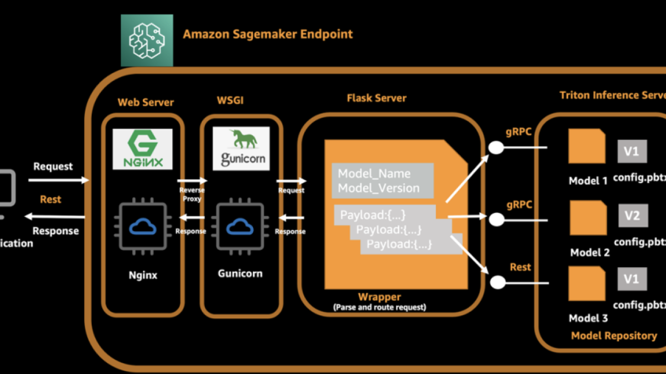
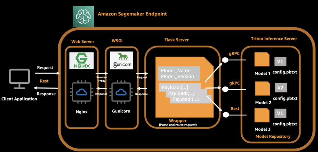
Let’s look at how SageMaker inference works. SageMaker invokes the hosting service by running a Docker container. The Docker container launches a RESTful inference server (such as Flask) to serve HTTP requests for inference. The inference server loads the model and listens to port 8080 providing external service. The client application sends a POST request to the SageMaker endpoint, SageMaker passes the request to the container, and returns the inference result from the container to the client.
In our architecture, we use NVIDIA Triton Inference Server, which provides concurrent runs of multiple models from different frameworks, and we use a Flask server to process client-side requests and dispatch these requests to the backend Triton server. While launching a Docker container, the Triton server and Flask server are started automatically. The Triton server loads multiple models and exposes ports 8000, 8001, and 8002 as gRPC, HTTP, and metrics server. The Flask server listens to 8080 ports and parses the original request and payload, and then invokes the local Triton backend via model name and version information. For the client side, it adds the model name and model version in the request in addition to the original payload, so that Flask is able to route the inference request to the correct model on Triton server.
The following diagram illustrates this process.
A complete API call from the client is as follows:
- The client assembles the request and initiates the request to a SageMaker endpoint.
- The Flask server receives and parses the request, and gets the model name, version, and payload.
- The Flask server assembles the request again and routes to the corresponding endpoint of the Triton server according to the model name and version.
- The Triton server runs an inference request and sends responses to the Flask server.
- The Flask server receives the response message, assembles the message again, and returns it to the client.
- The client receives and parses the response, and continues to subsequent business procedures.
In the following sections, we introduce the steps needed to prepare a model and build the TensorRT engine, prepare a Docker image, create a SageMaker endpoint, and verify the result.
Prepare models and build the engine
We demonstrate hosting three typical ML models in our solution: image classification (ResNet50), object detection (YOLOv5), and a natural language processing (NLP) model (BERT-base). NVIDIA Triton Inference Server supports multiple formats, including TensorFlow 1. x and 2. x, TensorFlow SavedModel, TensorFlow GraphDef, TensorRT, ONNX, OpenVINO, and PyTorch TorchScript.
The following table summarizes our model details.
| Model Name | Model Size | Format |
| ResNet50 | 52M | Tensor RT |
| YOLOv5 | 38M | Tensor RT |
| BERT-base | 133M | ONNX RT |
NVIDIA provides detailed documentation describing how to generate the TensorRT engine. To achieve best performance, the TensorRT engine must be built over the device. This means the build time and runtime require the same computer capacity. For example, a TensorRT engine built on a g4dn instance can’t be deployed on a g5 instance.
You can generate your own TensorRT engines according to your needs. For test purposes, we prepared sample codes and deployable models with the TensorRT engine. The source code is also available on GitHub.
Next, we use an Amazon Elastic Compute Cloud (Amazon EC2) G4dn instance to generate the TensorRT engine with the following steps. We use YOLOv5 as an example.
- Launch a G4dn.2xlarge EC2 instance with the Deep Learning AMI (Ubuntu 20.04) in the
us-east-1Region. - Open a terminal window and use the
sshcommand to connect to the instance. - Run the following commands one by one:
- Create a
config.pbtxtfile: - Create the following file structure and put the generated files in the appropriate location:
Test the TensorRT engine
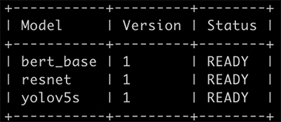
Before we deploy to SageMaker, we start a Triton server to verify these three models are configured correctly. Use the following command to start a Triton server and load the models:
If you receive the following prompt message, it means the Triton server is started correctly.
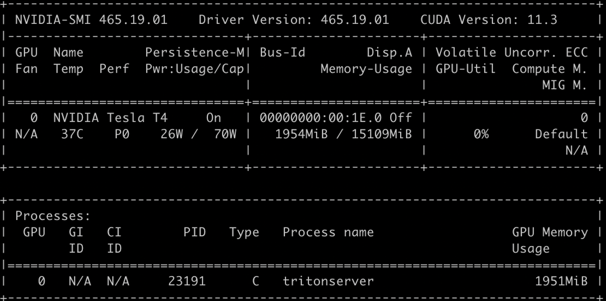
Enter nvidia-smi in the terminal to see GPU memory usage.
Client implementation for inference
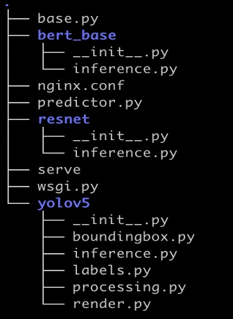
The file structure is as follows:
- serve – The wrapper that starts the inference server. The Python script starts the NGINX, Flask, and Triton server.
- predictor.py – The Flask implementation for
/pingand/invocationsendpoints, and dispatching requests. - wsgi.py – The startup shell for the individual server workers.
- base.py – The abstract method definition that each client requires to implement their inference method.
- client folder – One folder per client:
resnetbert_baseyolov5
- nginx.conf – The configuration for the NGINX primary server.
We define an abstract method to implement the inference interface, and each client implements this method:
The Triton server exposes an HTTP endpoint on port 8000, a gRPC endpoint on port 8001, and a Prometheus metrics endpoint on port 8002. The following is a sample ResNet client with a gRPC call. You can implement the HTTP interface or gRPC interface according to your use case.
In this architecture, the NGINX, Flask, and Triton servers should be started at the beginning. Edit the serve file and add a line to start the Triton server.
Build a Docker image and push the image to Amazon ECR
The Docker file code looks as follows:
The following table shows the cost for sharing one endpoint for three models using the preceding architecture. The total cost is about $676.8/month. From this result, we can conclude that you can save 30% in costs while also having 24/7 service from your endpoint.
| Model Name | Endpoint Running /Day | Instance Type | Cost/Month (us-east-1) |
| ResNet, YOLOv5, BERT | 24 hours | ml.g4dn.2xlarge | 0.94 * 24 * 30 = $676.8 |
Summary
In this post, we introduced an improved architecture in which multiple models share one endpoint in SageMaker. Under some conditions, this solution can help you save costs and improve resource utilization. It is suitable for business scenarios with low concurrency and latency-insensitive requirements.
To learn more about SageMaker and AI/ML solutions, refer to Amazon SageMaker.
References
- Use Triton Inference Server with Amazon SageMaker
- Achieve low-latency hosting for decision tree-based ML models on NVIDIA Triton Inference Server on Amazon SageMaker
- Deploy fast and scalable AI with NVIDIA Triton Inference Server in Amazon SageMaker
- NVIDIA Triton Inference Server
- YOLOv5
- Export to ONNX
- amazon-sagemaker-examples/sagemaker-triton GitHub repo
- Amazon SageMaker Pricing
About the authors
 Zheng Zhang is a Senior Specialist Solutions Architect in AWS, he focuses on helping customers accelerate model training, inference and deployment for machine learning solutions. He also has rich experience in large-scale distributed training, design AI/ML solutions.
 Yinuo He is an AI/ML specialist in AWS. She has experiences in designing and developing machine learning based products to provide better user experiences. She now works to help customers succeed in their ML journey.