The last few years have seen rapid development in the field of deep learning. Although hardware has improved, such as with the latest generation of accelerators from NVIDIA and Amazon, advanced machine learning (ML) practitioners still regularly encounter issues deploying their large deep learning models for applications such as natural language processing (NLP).
In an earlier post, we discussed capabilities and configurable settings in Amazon SageMaker model deployment that can make inference with these large models easier. Today, we announce a new Amazon SageMaker Deep Learning Container (DLC) that you can use to get started with large model inference in a matter of minutes. This DLC packages some of the most popular open-source libraries for model parallel inference, such as DeepSpeed and Hugging Face Accelerate.
In this post, we use a new SageMaker large model inference DLC to deploy two of the most popular large NLP models: BigScience’s BLOOM-176B and Meta’s OPT-30B from the Hugging Face repository. In particular, we use Deep Java Library (DJL) serving and tensor parallelism techniques from DeepSpeed to achieve 0.1 second latency per token in a text generation use case.
You can find our complete example notebooks in our GitHub repository.
Large model inference techniques
Language models have recently exploded in both size and popularity. With easy access from model zoos such as Hugging Face and improved accuracy and performance in NLP tasks such as classification and text generation, practitioners are increasingly reaching for these large models. However, large models are often too big to fit within the memory of a single accelerator. For example, the BLOOM-176B model can require more than 350 gigabytes of accelerator memory, which far exceeds the capacity of hardware accelerators available today. This necessitates the use of model parallel techniques from libraries like DeepSpeed and Hugging Face Accelerate to distribute a model across multiple accelerators for inference. In this post, we use the SageMaker large model inference container to generate and compare latency and throughput performance using these two open-source libraries.
DeepSpeed and Accelerate use different techniques to optimize large language models for inference. The key difference is DeepSpeed’s use of optimized kernels. These kernels can dramatically improve inference latency by reducing bottlenecks in the computation graph of the model. Optimized kernels can be difficult to develop and are typically specific to a particular model architecture; DeepSpeed supports popular large models such as OPT and BLOOM with these optimized kernels. In contrast, Hugging Face’s Accelerate library doesn’t include optimized kernels at the time of writing. As we discuss in our results section, this difference is responsible for much of the performance edge that DeepSpeed has over Accelerate.
A second difference between DeepSpeed and Accelerate is the type of model parallelism. Accelerate uses pipeline parallelism to partition a model between the hidden layers of a model, whereas DeepSpeed uses tensor parallelism to partition the layers themselves. Pipeline parallelism is a flexible approach that supports more model types and can improve throughput when larger batch sizes are used. Tensor parallelism requires more communication between GPUs because model layers can be spread across multiple devices, but can improve inference latency by engaging multiple GPUs simultaneously. You can learn more about parallelism techniques in Introduction to Model Parallelism and Model Parallelism.
Solution overview
To effectively host large language models, we need features and support in the following key areas:
- Building and testing solutions – Given the iterative nature of ML development, we need the ability to build, rapidly iterate, and test how the inference endpoint will behave when these models are hosted, including the ability to fail fast. These models can typically be hosted only on larger instances like p4dn or g5, and given the size of the models, it can take a while to spin up an inference instance and run any test iteration. Local testing usually has constraints because you need a similar instance in size to test, and these models aren’t easy to obtain.
- Deploying and running at scale – The model files need to be loaded onto the inference instances, which presents a challenge in itself given the size. Tar / Un-Tar as an example for the Bloom-176B takes about 1 hour to create and another hour to load. We need an alternate mechanism to allow easy access to the model files.
- Loading the model as singleton – For a multi-worker process, we need to ensure the model gets loaded only once so we don’t run into race conditions and further spend unnecessary resources. In this post, we show a way to load directly from Amazon Simple Storage Service (Amazon S3). However, this only works if we use the default settings of the DJL. Furthermore, any scaling of the endpoints needs to be able to spin up in a few minutes, which calls for reconsidering how the models might be loaded and distributed.
- Sharding frameworks – These models typically need to be , usually by a tensor parallelism mechanism or by pipeline sharding as the typical sharding techniques, and we have advanced concepts like ZeRO sharding built on top of tensor sharding. For more information about sharding techniques, refer to Model Parallelism. To achieve this, we can have various combinations and use frameworks from NIVIDIA, DeepSpeed, and others. This needs the ability to test BYOC or use 1P containers and iterate over solutions and run benchmarking tests. You might also want to test various hosting options like asynchronous, serverless, and others.
- Hardware selection – Your choice in hardware is determined by all the aforementioned points and further traffic patterns, use case needs, and model sizes.
In this post, we use DeepSpeed’s optimized kernels and tensor parallelism techniques to host BLOOM-176B and OPT-30B on SageMaker. We also compare results from Accelerate to demonstrate the performance benefits of optimized kernels and tensor parallelism. For more information on DeepSpeed and Accelerate, refer to DeepSpeed Inference: Enabling Efficient Inference of Transformer Models at Unprecedented Scale and Incredibly Fast BLOOM Inference with DeepSpeed and Accelerate.
We use DJLServing as the model serving solution in this example. DJLServing is a high-performance universal model serving solution powered by the Deep Java Library (DJL) that is programming language agnostic. To learn more about the DJL and DJLServing, refer to Deploy large models on Amazon SageMaker using DJLServing and DeepSpeed model parallel inference.
It’s worth noting that optimized kernels can result in precision changes and a modified computation graph, which could theoretically result in changed model behavior. Although this could occasionally change the inference outcome, we do not expect these differences to materially impact the basic evaluation metrics of a model. Nevertheless, practitioners are advised to confirm the model outputs are as expected when using these kernels.
The following steps demonstrate how to deploy a BLOOM-176B model in SageMaker using DJLServing and a SageMaker large model inference container. The complete example is also available in our GitHub repository.
Using the DJLServing SageMaker DLC image
Use the following code to use the DJLServing SageMaker DLC image after replacing the region with your specific region you are running the notebook in:
Create our model file
First, we create a file called serving.properties that contains only one line of code. This tells the DJL model server to use the DeepSpeed engine. The file contains the following code:
serving.properties is a file defined by DJLServing that is used to configure per-model configuration.
Next, we create our model.py file, which defines the code needed to load and then serve the model. In our code, we read in the TENSOR_PARALLEL_DEGREE environment variable (the default value is 1). This sets the number of devices over which the tensor parallel modules are distributed. Note that DeepSpeed provides a few built-in partition definitions, including one for BLOOM models. We use it by specifying replace_method and relpace_with_kernel_inject. If you have a customized model and need DeepSpeed to partition effectively, you need to change relpace_with_kernel_inject to false and add injection_policy to make the runtime partition work. For more information, refer to Initializing for Inference. For our example, we used the pre-partitioned BLOOM model on DeepSpeed.
Secondly, in the model.py file, we also load the model from Amazon S3 after the endpoint has been spun up. The model is loaded into the /tmp space on the container because SageMaker maps the /tmp to the Amazon Elastic Block Store (Amazon EBS) volume that is mounted when we specify the endpoint creation parameter VolumeSizeInGB. For instances like p4dn, which come pre-built with the volume instance, we can continue to leverage the /tmp on the container. See the following code:
DJLServing manages the runtime installation on any pip packages defined in requirement.txt. This file will have:
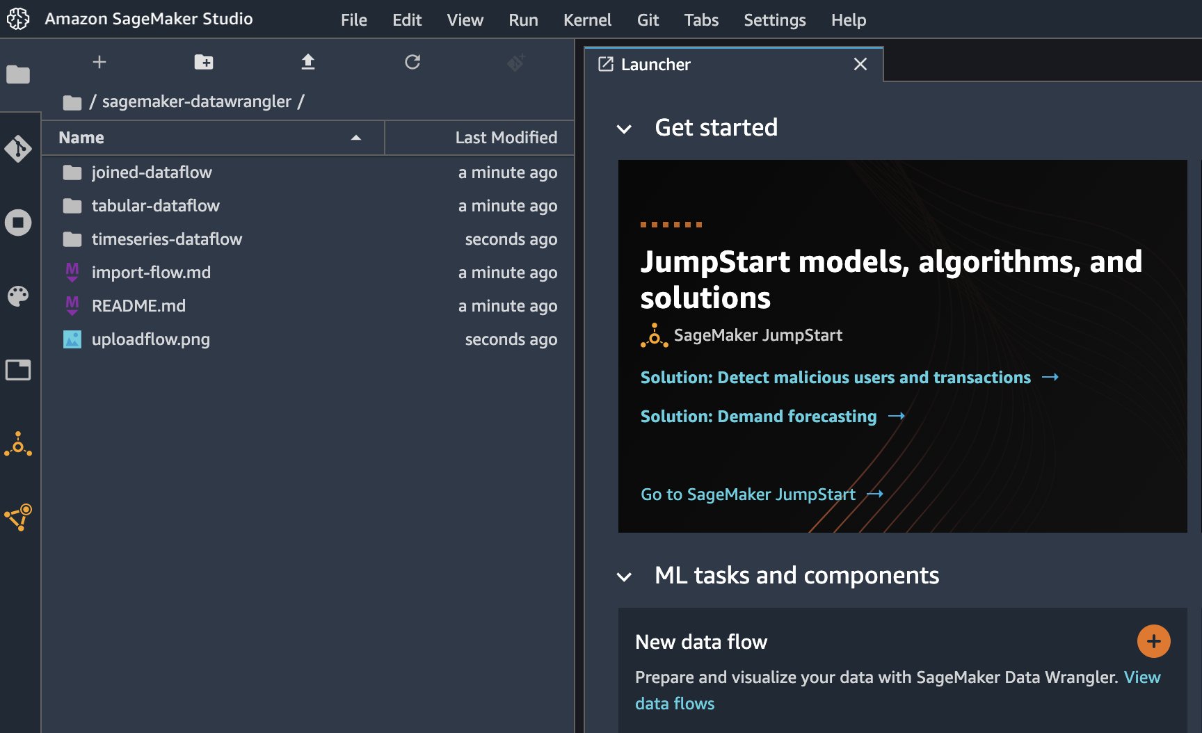
We have created a directory called code and the model.py, serving.properties, and requirements.txt files are already created in this directory. To view the files, you can run the following code from the terminal:
The following figure shows the structure of the model.tar.gz.

Lastly, we create the model file and upload it to Amazon S3:
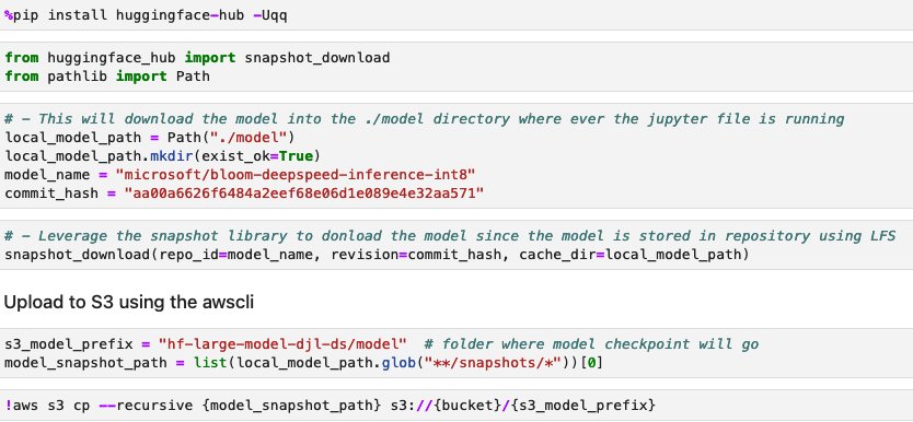
Download and store the model from Hugging Face (Optional)
We have provided the steps in this section in case you want to download the model to Amazon S3 and use it from there. The steps are provided in the Jupyter file on GitHub. The following screenshot shows a snapshot of the steps.
Create a SageMaker model
We now create a SageMaker model. We use the Amazon Elastic Container Registry (Amazon ECR) image provided by and the model artifact from the previous step to create the SageMaker model. In the model setup, we configure TENSOR_PARALLEL_DEGREE=8, which means the model is partitioned along 8 GPUs. See the following code:
After you run the preceding cell in the Jupyter file, you see output similar to the following:
Create a SageMaker endpoint
You can use any instances with multiple GPUs for testing. In this demo, we use a p4d.24xlarge instance. In the following code, note how we set the ModelDataDownloadTimeoutInSeconds, ContainerStartupHealthCheckTimeoutInSeconds, and VolumeSizeInGB parameters to accommodate the large model size. The VolumeSizeInGB parameter is applicable to GPU instances supporting the EBS volume attachment.
Lastly, we create a SageMaker endpoint:
You see it printed out in the following code:
Starting the endpoint might take a while. You can try a few more times if you run into the InsufficientInstanceCapacity error, or you can raise a request to AWS to increase the limit in your account.
Performance tuning
If you intend to use this post and accompanying notebook with a different model, you may want to explore some of the tunable parameters that SageMaker, DeepSpeed, and the DJL offer. Iteratively experimenting with these parameters can have a material impact on the latency, throughput, and cost of your hosted large model. To learn more about tuning parameters such as number of workers, degree of tensor parallelism, job queue size, and others, refer to DJL Serving configurations and Deploy large models on Amazon SageMaker using DJLServing and DeepSpeed model parallel inference.
Results
In this post, we used DeepSpeed to host BLOOM-176B and OPT-30B on SageMaker ML instances. The following table summarizes our performance results, including a comparison with Hugging Face’s Accelerate. Latency reflects the number of milliseconds it takes to produce a 256-token string four times (batch_size=4) from the model. Throughput reflects the number of tokens produced per second for each test. For Hugging Face Accelerate, we used the library’s default loading with GPU memory mapping. For DeepSpeed, we used its faster checkpoint loading mechanism.
| Model | Library | Model Precision | Batch Size | Parallel Degree | Instance | Time to Load (s) |
Latency (4 x 256 Token Output) | . | ||
| . | . | . | . | . | . | . | P50 (ms) |
P90 (ms) |
P99 (ms) |
Throughput (tokens/sec) |
| BLOOM-176B | DeepSpeed | INT8 | 4 | 8 | p4d.24xlarge | 74.9 | 27,564 | 27,580 | 32,179 | 37.1 |
| BLOOM-176B | Accelerate | INT8 | 4 | 8 | p4d.24xlarge | 669.4 | 92,694 | 92,735 | 103,292 | 11.0 |
| OPT-30B | DeepSpeed | FP16 | 4 | 4 | g5.24xlarge | 239.4 | 11,299 | 11,302 | 11,576 | 90.6 |
| OPT-30B | Accelerate | FP16 | 4 | 4 | g5.24xlarge | 533.8 | 63,734 | 63,737 | 67,605 | 16.1 |
From a latency perspective, DeepSpeed is about 3.4 times faster for BLOOM-176B and 5.6 times faster for OPT-30B than Accelerate. DeepSpeed’s optimized kernels are responsible for much of this difference in latency. Given these results, we recommend using DeepSpeed over Accelerate if your model of choice is supported.
It’s also worth noting that model loading times with DeepSpeed were much shorter, making it a better option if you anticipate needing to quickly scale up your number of endpoints. Accelerate’s more flexible pipeline parallelism technique may be a better option if you have models or model precisions that aren’t supported by DeepSpeed.
These results also demonstrate the difference in latency and throughput of different model sizes. In our tests, OPT-30B generates 2.4 times the number of tokens per unit time than BLOOM-176B on an instance type that is more than three times cheaper. On a price per unit throughput basis, OPT-30B on a g5.24xl instance is 8.9 times better than BLOOM-176B on a p4d.24xl instance. If you have strict latency, throughput, or cost limitations, consider using the smallest model possible that will still achieve functional requirements.
Clean up
As part of best practices it is always recommended to delete idle instances. The below code shows you how to delete the instances.
Optionally delete the model check point from your S3
Conclusion
In this post, we demonstrated how to use SageMaker large model inference containers to host two large language models, BLOOM-176B and OPT-30B. We used DeepSpeed’s model parallel techniques with multiple GPUs on a single SageMaker ML instance.
For more details about Amazon SageMaker and its large model inference capabilities, refer to Amazon SageMaker now supports deploying large models through configurable volume size and timeout quotas and Real-time inference.
About the authors
 Simon Zamarin is an AI/ML Solutions Architect whose main focus is helping customers extract value from their data assets. In his spare time, Simon enjoys spending time with family, reading sci-fi, and working on various DIY house projects.
 Rupinder Grewal is a Sr Ai/ML Specialist Solutions Architect with AWS. He currently focuses on serving of models and MLOps on SageMaker. Prior to this role he has worked as Machine Learning Engineer building and hosting models. Outside of work he enjoys playing tennis and biking on mountain trails.
 Frank Liu is a Software Engineer for AWS Deep Learning. He focuses on building innovative deep learning tools for software engineers and scientists. In his spare time, he enjoys hiking with friends and family.
 Alan Tan is a Senior Product Manager with SageMaker leading efforts on large model inference. He’s passionate about applying Machine Learning to the area of Analytics. Outside of work, he enjoys the outdoors.
 Dhawal Patel is a Principal Machine Learning Architect at AWS. He has worked with organizations ranging from large enterprises to mid-sized startups on problems related to distributed computing, and Artificial Intelligence. He focuses on Deep learning including NLP and Computer Vision domains. He helps customers achieve high performance model inference on SageMaker.
 Qing Lan is a Software Development Engineer in AWS. He has been working on several challenging products in Amazon, including high performance ML inference solutions and high performance logging system. Qing’s team successfully launched the first Billion-parameter model in Amazon Advertising with very low latency required. Qing has in-depth knowledge on the infrastructure optimization and Deep Learning acceleration.
 Qingwei Li is a Machine Learning Specialist at Amazon Web Services. He received his Ph.D. in Operations Research after he broke his advisor’s research grant account and failed to deliver the Nobel Prize he promised. Currently he helps customers in the financial service and insurance industry build machine learning solutions on AWS. In his spare time, he likes reading and teaching.
 Robert Van Dusen is a Senior Product Manager with Amazon SageMaker. He leads deep learning model optimization for applications such as large model inference.
 Siddharth Venkatesan is a Software Engineer in AWS Deep Learning. He currently focusses on building solutions for large model inference. Prior to AWS he worked in the Amazon Grocery org building new payment features for customers world-wide. Outside of work, he enjoys skiing, the outdoors, and watching sports.