Machine learning (ML) models are taking the world by storm. Their performance relies on using the right training data and choosing the right model and algorithm. But it doesn’t end here. Typically, algorithms defer some design decisions to the ML practitioner to adopt for their specific data and task. These deferred design decisions manifest themselves as hyperparameters.
What does that name mean? The result of ML training, the model, can be largely seen as a collection of parameters that are learned during training. Therefore, the parameters that are used to configure the ML training process are then called hyperparameters—parameters describing the creation of parameters. At any rate, they are of very practical use, such as the number of epochs to train, the learning rate, the max depth of a decision tree, and so forth. And we pay much attention to them because they have a major impact on the ultimate performance of your model.
Just like turning a knob on a radio receiver to find the right frequency, each hyperparameter should be carefully tuned to optimize performance. Searching the hyperparameter space for the optimal values is referred to as hyperparameter tuning or hyperparameter optimization (HPO), and should result in a model that gives accurate predictions.
In this post, we set up and run our first HPO job using Amazon SageMaker Automatic Model Tuning (AMT). We learn about the methods available to explore the results, and create some insightful visualizations of our HPO trials and the exploration of the hyperparameter space!
Amazon SageMaker Automatic Model Tuning
As an ML practitioner using SageMaker AMT, you can focus on the following:
- Providing a training job
- Defining the right objective metric matching your task
- Scoping the hyperparameter search space
SageMaker AMT takes care of the rest, and you don’t need to think about the infrastructure, orchestrating training jobs, and improving hyperparameter selection.
Let’s start by using SageMaker AMT for our first simple HPO job, to train and tune an XGBoost algorithm. We want your AMT journey to be hands-on and practical, so we have shared the example in the following GitHub repository. This post covers the 1_tuning_of_builtin_xgboost.ipynb notebook.
In an upcoming post, we’ll extend the notion of just finding the best hyperparameters and include learning about the search space and to what hyperparameter ranges a model is sensitive. We’ll also show how to turn a one-shot tuning activity into a multi-step conversation with the ML practitioner, to learn together. Stay tuned (pun intended)!
Prerequisites
This post is for anyone interested in learning about HPO and doesn’t require prior knowledge of the topic. Basic familiarity with ML concepts and Python programming is helpful though. For the best learning experience, we highly recommend following along by running each step in the notebook in parallel to reading this post. And at the end of the notebook, you also get to try out an interactive visualization that makes the tuning results come alive.
Solution overview
We’re going to build an end-to-end setup to run our first HPO job using SageMaker AMT. When our tuning job is complete, we look at some of the methods available to explore the results, both via the AWS Management Console and programmatically via the AWS SDKs and APIs.
First, we familiarize ourselves with the environment and SageMaker Training by running a standalone training job, without any tuning for now. We use the XGBoost algorithm, one of many algorithms provided as a SageMaker built-in algorithm (no training script required!).
We see how SageMaker Training operates in the following ways:
- Starts and stops an instance
- Provisions the necessary container
- Copies the training and validation data onto the instance
- Runs the training
- Collects metrics and logs
- Collects and stores the trained model
Then we move to AMT and run an HPO job:
- We set up and launch our tuning job with AMT
- We dive into the methods available to extract detailed performance metrics and metadata for each training job, which enables us to learn more about the optimal values in our hyperparameter space
- We show you how to view the results of the trials
- We provide you with tools to visualize data in a series of charts that reveal valuable insights into our hyperparameter space
Train a SageMaker built-in XGBoost algorithm
It all starts with training a model. In doing so, we get a sense of how SageMaker Training works.
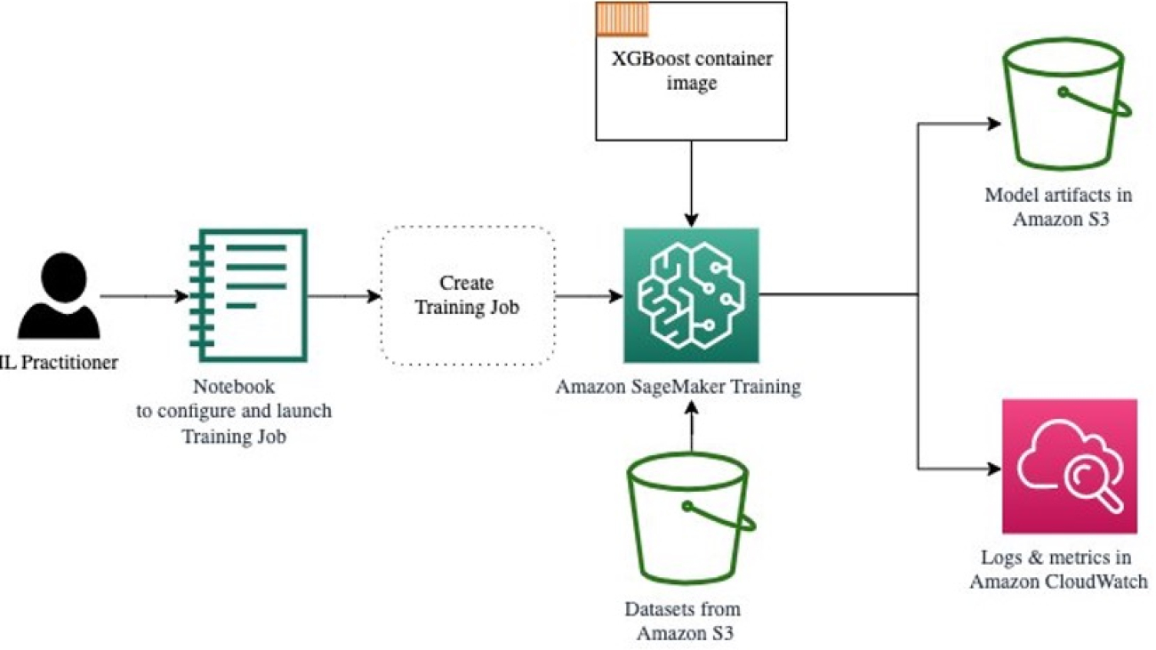
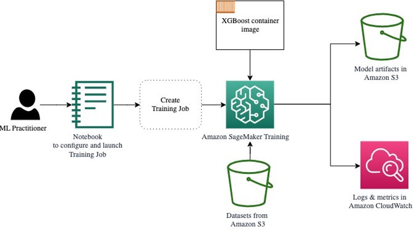
We want to take advantage of the speed and ease of use offered by the SageMaker built-in algorithms. All we need are a few steps to get started with training:
- Prepare and load the data – We download and prepare our dataset as input for XGBoost and upload it to our Amazon Simple Storage Service (Amazon S3) bucket.
- Select our built-in algorithm’s image URI – SageMaker uses this URI to fetch our training container, which in our case contains a ready-to-go XGBoost training script. Several algorithm versions are supported.
- Define the hyperparameters – SageMaker provides an interface to define the hyperparameters for our built-in algorithm. These are the same hyperparameters as used by the open-source version.
- Construct the estimator – We define the training parameters such as instance type and number of instances.
- Call the fit() function – We start our training job.
The following diagram shows how these steps work together.
Provide the data
To run ML training, we need to provide data. We provide our training and validation data to SageMaker via Amazon S3.
In our example, for simplicity, we use the SageMaker default bucket to store our data. But feel free to customize the following values to your preference:
sm_sess = sagemaker.session.Session([..])

BUCKET = sm_sess.default_bucket()
PREFIX = 'amt-visualize-demo'
output_path = f's3://{BUCKET}/{PREFIX}/output'
In the notebook, we use a public dataset and store the data locally in the data directory. We then upload our training and validation data to Amazon S3. Later, we also define pointers to these locations to pass them to SageMaker Training.
# acquire and prepare the data (not shown here)
# store the data locally
[..]
train_data.to_csv('data/train.csv', index=False, header=False)
valid_data.to_csv('data/valid.csv', index=False, header=False)
[..]
# upload the local files to S3
boto_sess.resource('s3').Bucket(BUCKET).Object(os.path.join(PREFIX, 'data/train/train.csv')).upload_file('data/train.csv')
boto_sess.resource('s3').Bucket(BUCKET).Object(os.path.join(PREFIX, 'data/valid/valid.csv')).upload_file('data/valid.csv')
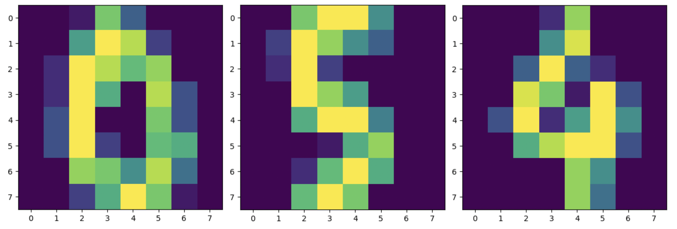
In this post, we concentrate on introducing HPO. For illustration, we use a specific dataset and task, so that we can obtain measurements of objective metrics that we then use to optimize the selection of hyperparameters. However, for the overall post neither the data nor the task matter. To present you with a complete picture, let us briefly describe what we do: we train an XGBoost model that should classify handwritten digits from the
Optical Recognition of Handwritten Digits Data Set [1] via Scikit-learn. XGBoost is an excellent algorithm for structured data and can even be applied to the Digits dataset. The values are 8×8 images, as in the following example showing a
0 a
5 and a
4.
Select the XGBoost image URI
After choosing our built-in algorithm (XGBoost), we must retrieve the image URI and pass this to SageMaker to load onto our training instance. For this step, we review the available versions. Here we’ve decided to use version 1.5.1, which offers the latest version of the algorithm. Depending on the task, ML practitioners may write their own training script that, for example, includes data preparation steps. But this isn’t necessary in our case.
If you want to write your own training script, then stay tuned, we’ve got you covered in our next post! We’ll show you how to run SageMaker Training jobs with your own custom training scripts.
For now, we need the correct image URI by specifying the algorithm, AWS Region, and version number:
xgboost_container = sagemaker.image_uris.retrieve('xgboost', region, '1.5-1')
That’s it. Now we have a reference to the XGBoost algorithm.
Define the hyperparameters
Now we define our hyperparameters. These values configure how our model will be trained, and eventually influence how the model performs against the objective metric we’re measuring against, such as accuracy in our case. Note that nothing about the following block of code is specific to SageMaker. We’re actually using the open-source version of XGBoost, just provided by and optimized for SageMaker.
Although each of these hyperparameters are configurable and adjustable, the objective metric multi:softmax is determined by our dataset and the type of problem we’re solving for. In our case, the Digits dataset contains multiple labels (an observation of a handwritten digit could be 0 or 1,2,3,4,5,6,7,8,9), meaning it is a multi-class classification problem.
hyperparameters = {
    'num_class': 10,
    'max_depth': 5,
    'eta':0.2,
    'alpha': 0.2,
    'objective':'multi:softmax',
    'eval_metric':'accuracy',
    'num_round':200,
    'early_stopping_rounds': 5
}
For more information about the other hyperparameters, refer to XGBoost Hyperparameters.
Construct the estimator
We configure the training on an estimator object, which is a high-level interface for SageMaker Training.
Next, we define the number of instances to train on, the instance type (CPU-based or GPU-based), and the size of the attached storage:
estimator = sagemaker.estimator.Estimator(
    image_uri=xgboost_container,
    hyperparameters=hyperparameters,
    role=role,
    instance_count=1,
    instance_type='ml.m5.large',
    volume_size=5, # 5 GB
    output_path=output_path
)
We now have the infrastructure configuration that we need to get started. SageMaker Training will take care of the rest.
Call the fit() function
Remember the data we uploaded to Amazon S3 earlier? Now we create references to it:
s3_input_train = TrainingInput(s3_data=f's3://{BUCKET}/{PREFIX}/data/train', content_type='csv')
s3_input_valid = TrainingInput(s3_data=f's3://{BUCKET}/{PREFIX}/data/valid', content_type='csv')
A call to fit() launches our training. We pass in the references to the training data we just created to point SageMaker Training to our training and validation data:
estimator.fit({'train': s3_input_train, 'validation': s3_input_valid})
Note that to run HPO later on, we don’t actually need to call fit() here. We just need the estimator object later on for HPO, and could just jump to creating our HPO job. But because we want to learn about SageMaker Training and see how to run a single training job, we call it here and review the output.
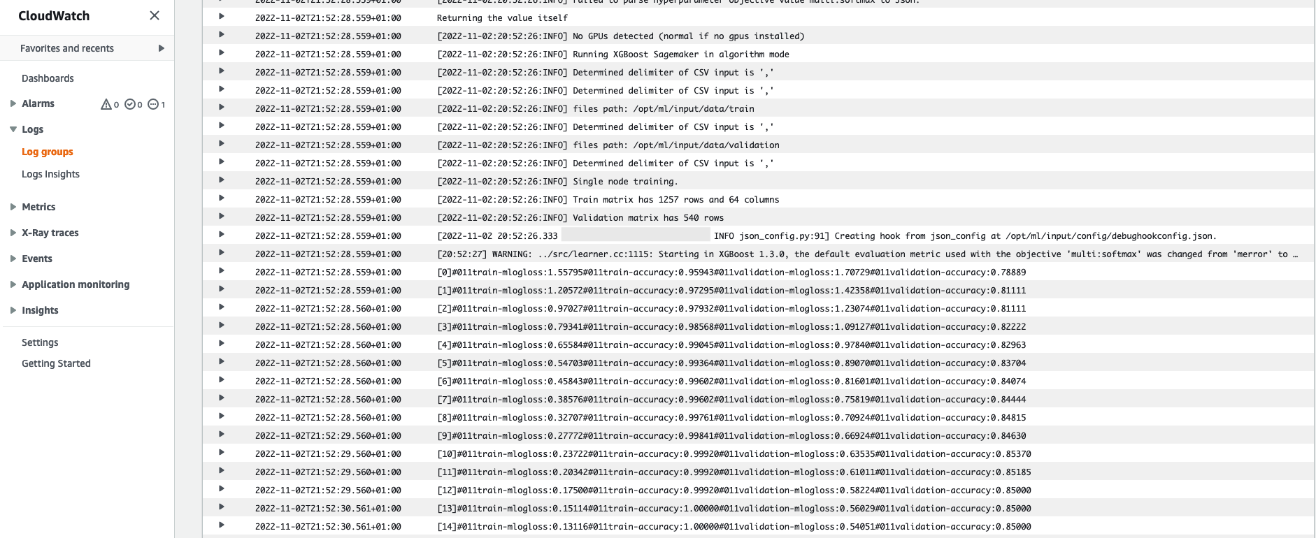
After the training starts, we start to see the output below the cells, as shown in the following screenshot. The output is available in Amazon CloudWatch as well as in this notebook.
The black text is log output from SageMaker itself, showing the steps involved in training orchestration, such as starting the instance and loading the training image. The blue text is output directly from the training instance itself. We can observe the process of loading and parsing the training data, and visually see the training progress and the improvement in the objective metric directly from the training script running on the instance.
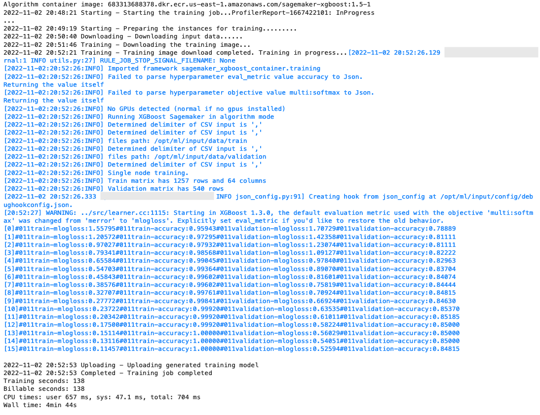
Also note that at the end of the output job, the training duration in seconds and billable seconds are shown.
Finally, we see that SageMaker uploads our training model to the S3 output path defined on the estimator object. The model is ready to be deployed for inference.
In a future post, we’ll create our own training container and define our training metrics to emit. You’ll see how SageMaker is agnostic of what container you pass it for training. This is very handy for when you want to get started quickly with a built-in algorithm, but then later decide to pass your own custom training script!
Inspect current and previous training jobs
So far, we have worked from our notebook with our code and submitted training jobs to SageMaker. Let’s switch perspectives and leave the notebook for a moment to check out what this looks like on the SageMaker console.
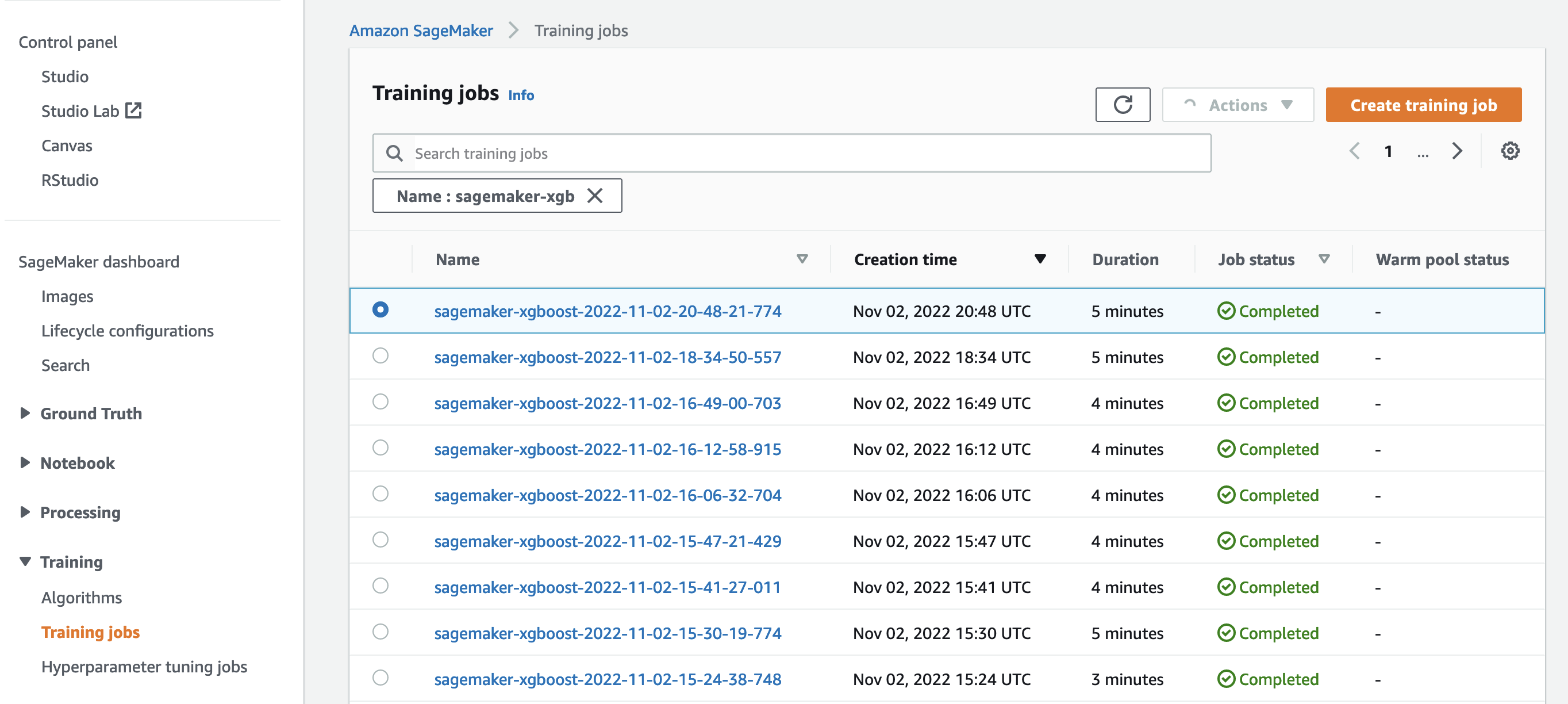
SageMaker keeps a historic record of training jobs it ran, their configurations such as hyperparameters, algorithms, data input, the billable time, and the results. In the list in the preceding screenshot, you see the most recent training jobs filtered for XGBoost. The highlighted training job is the job we just trained in the notebook, whose output you saw earlier. Let’s dive into this individual training job to get more information.
The following screenshot shows the console view of our training job.
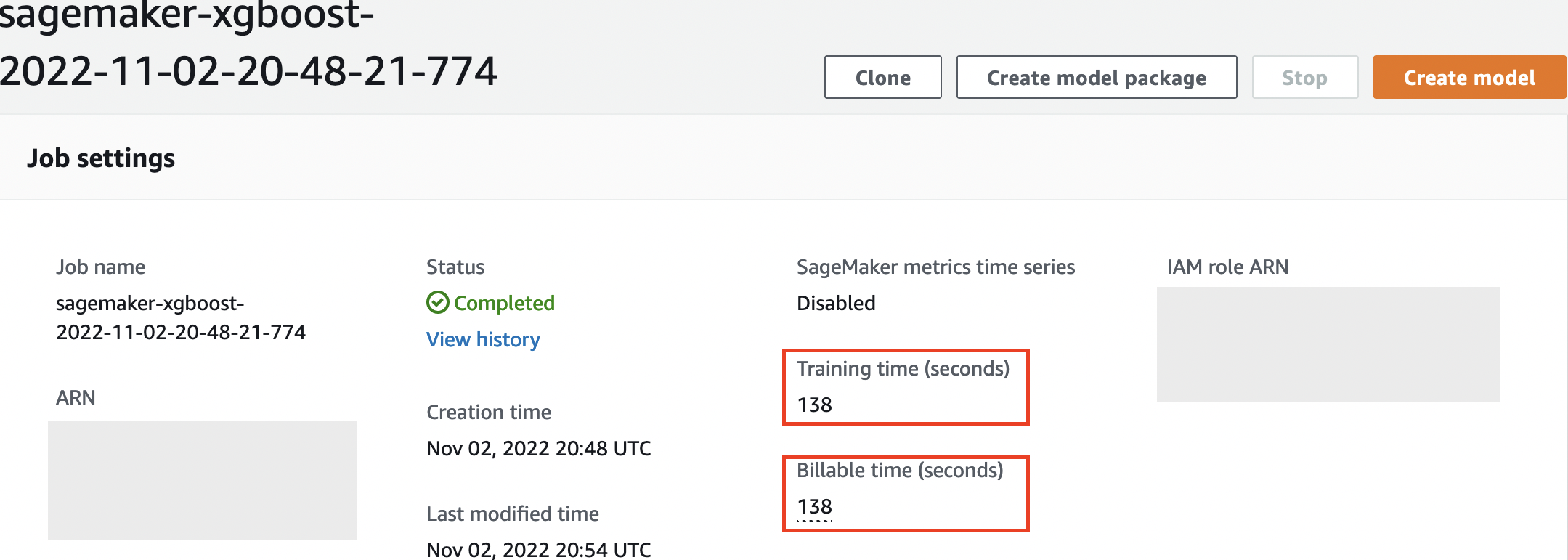
We can review the information we received as cell output to our fit() function in the individual training job within the SageMaker console, along with the parameters and metadata we defined in our estimator.
Recall the log output from the training instance we saw earlier. We can access the logs of our training job here too, by scrolling to the Monitor section and choosing View logs.

This shows us the instance logs inside CloudWatch.
Also remember the hyperparameters we specified in our notebook for the training job. We see them here in the same UI of the training job as well.
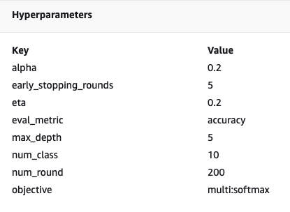
In fact, the details and metadata we specified earlier for our training job and estimator can be found on this page on the SageMaker console. We have a helpful record of the settings used for the training, such as what training container was used and the locations of the training and validation datasets.
You might be asking at this point, why exactly is this relevant for hyperparameter optimization? It’s because you can search, inspect, and dive deeper into those HPO trials that we’re interested in. Maybe the ones with the best results, or the ones that show interesting behavior. We’ll leave it to you what you define as “interesting.” It gives us a common interface for inspecting our training jobs, and you can use it with SageMaker Search.
Although SageMaker AMT orchestrates the HPO jobs, the HPO trials are all launched as individual SageMaker Training jobs and can be accessed as such.
With training covered, let’s get tuning!
Train and tune a SageMaker built-in XGBoost algorithm
To tune our XGBoost model, we’re going to reuse our existing hyperparameters and define ranges of values we want to explore for them. Think of this as extending the borders of exploration within our hyperparameter search space. Our tuning job will sample from the search space and run training jobs for new combinations of values. The following code shows how to specify the hyperparameter ranges that SageMaker AMT should sample from:
from sagemaker.tuner import IntegerParameter, ContinuousParameter, HyperparameterTuner

hpt_ranges = {
    'alpha': ContinuousParameter(0.01, .5),
    'eta': ContinuousParameter(0.1, .5),
    'min_child_weight': ContinuousParameter(0., 2.),
    'max_depth': IntegerParameter(1, 10)
}
The ranges for an individual hyperparameter are specified by their type, like ContinuousParameter. For more information and tips on choosing these parameter ranges, refer to Tune an XGBoost Model.
We haven’t run any experiments yet, so we don’t know the ranges of good values for our hyperparameters. Therefore, we start with an educated guess, using our knowledge of algorithms and our documentation of the hyperparameters for the built-in algorithms. This defines a starting point to define the search space.
Then we run a tuning job sampling from hyperparameters in the defined ranges. As a result, we can see which hyperparameter ranges yield good results. With this knowledge, we can refine the search space’s boundaries by narrowing or widening which hyperparameter ranges to use. We demonstrate how to learn from the trials in the next and final section, where we investigate and visualize the results.
In our next post, we’ll continue our journey and dive deeper. In addition, we’ll learn that there are several strategies that we can use to explore our search space. We’ll run subsequent HPO jobs to find even more performant values for our hyperparameters, while comparing these different strategies. We’ll also see how to run a warm start with SageMaker AMT to use the knowledge gained from previously explored search spaces in our exploration beyond those initial boundaries.
For this post, we focus on how to analyze and visualize the results of a single HPO job using the Bayesian search strategy, which is likely to be a good starting point.
If you follow along in the linked notebook, note that we pass the same estimator that we used for our single, built-in XGBoost training job. This estimator object acts as a template for new training jobs that AMT creates. AMT will then vary the hyperparameters inside the ranges we defined.
By specifying that we want to maximize our objective metric, validation:accuracy, we’re telling SageMaker AMT to look for these metrics in the training instance logs and pick hyperparameter values that it believes will maximize the accuracy metric on our validation data. We picked an appropriate objective metric for XGBoost from our documentation.
Additionally, we can take advantage of parallelization with max_parallel_jobs. This can be a powerful tool, especially for strategies whose trials are selected independently, without considering (learning from) the outcomes of previous trials. We’ll explore these other strategies and parameters further in our next post. For this post, we use Bayesian, which is an excellent default strategy.
We also define max_jobs to define how many trials to run in total. Feel free to deviate from our example and use a smaller number to save money.
n_jobs = 50
n_parallel_jobs = 3

tuner_parameters = {
    'estimator': estimator, # The same estimator object we defined above
    'base_tuning_job_name': 'bayesian',
    'objective_metric_name': 'validation:accuracy',
    'objective_type': 'Maximize',
    'hyperparameter_ranges': hpt_ranges,
    'strategy': 'Bayesian',
    'max_jobs': n_jobs,
    'max_parallel_jobs': n_parallel_jobs
}
We once again call fit(), the same way as when we launched a single training job earlier in the post. But this time on the tuner object, not the estimator object. This kicks off the tuning job, and in turn AMT starts training jobs.
tuner = HyperparameterTuner(**tuner_parameters)
tuner.fit({'train': s3_input_train, 'validation': s3_input_valid}, wait=False)
tuner_name = tuner.describe()['HyperParameterTuningJobName']
print(f'tuning job submitted: {tuner_name}.')
The following diagram expands on our previous architecture by including HPO with SageMaker AMT.
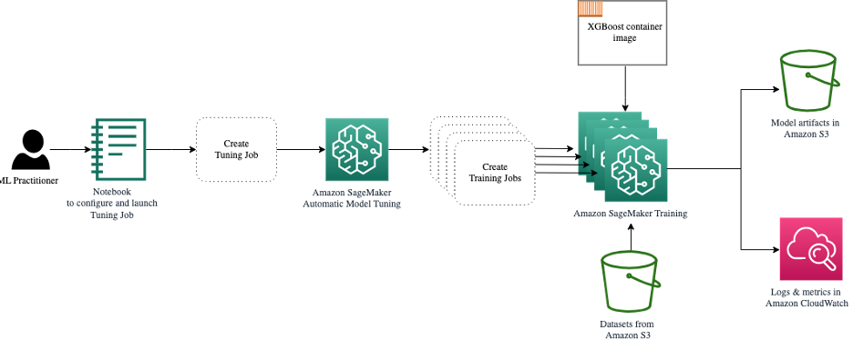
We see that our HPO job has been submitted. Depending on the number of trials, defined by n_jobs and the level of parallelization, this may take some time. For our example, it may take up to 30 minutes for 50 trials with only a parallelization level of 3.
tuning job submitted: bayesian-221102-2053.
When this tuning job is finished, let’s explore the information available to us on the SageMaker console.
Investigate AMT jobs on the console
Let’s find our tuning job on the SageMaker console by choosing Training in the navigation pane and then Hyperparameter tuning jobs. This gives us a list of our AMT jobs, as shown in the following screenshot. Here we locate our bayesian-221102-2053 tuning job and find that it’s now complete.
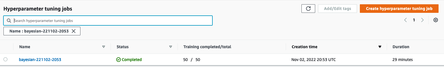
Let’s have a closer look at the results of this HPO job.
We have explored extracting the results programmatically in the notebook. First via the SageMaker Python SDK, which is a higher level open-source Python library, providing a dedicated API to SageMaker. Then through Boto3, which provides us with lower-level APIs to SageMaker and other AWS services.
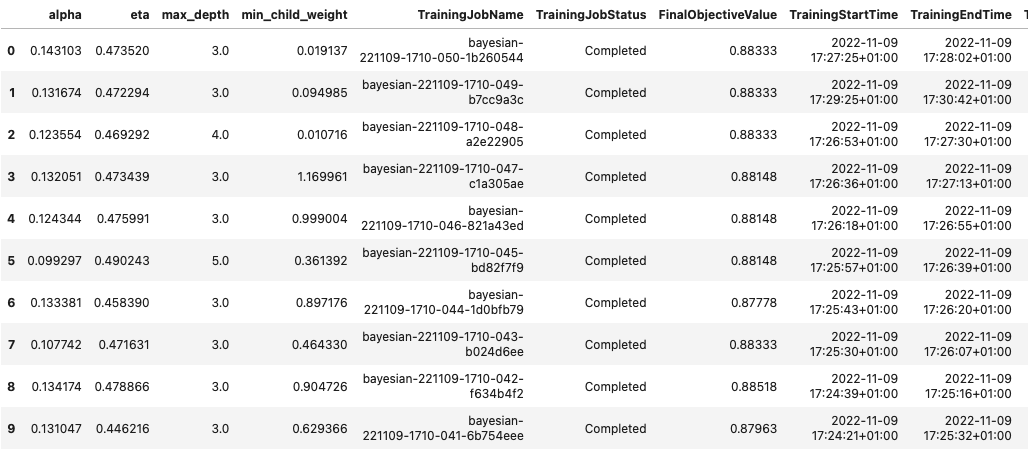
Using the SageMaker Python SDK, we can obtain the results of our HPO job:
sagemaker.HyperparameterTuningJobAnalytics(tuner_name).dataframe()[:10]
This allowed us to analyze the results of each of our trials in a Pandas DataFrame, as seen in the following screenshot.
Now let’s switch perspectives again and see what the results look like on the SageMaker console. Then we’ll look at our custom visualizations.
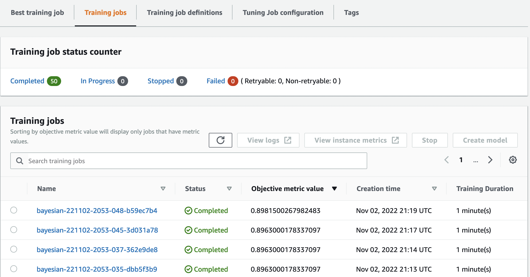
On the same page, choosing our bayesian-221102-2053 tuning job provides us with a list of trials that were run for our tuning job. Each HPO trial here is a SageMaker Training job. Recall earlier when we trained our single XGBoost model and investigated the training job in the SageMaker console. We can do the same thing for our trials here.
As we investigate our trials, we see that bayesian-221102-2053-048-b59ec7b4 created the best performing model, with a validation accuracy of approximately 89.815%. Let’s explore what hyperparameters led to this performance by choosing the Best training job tab.
We can see a detailed view of the best hyperparameters evaluated.
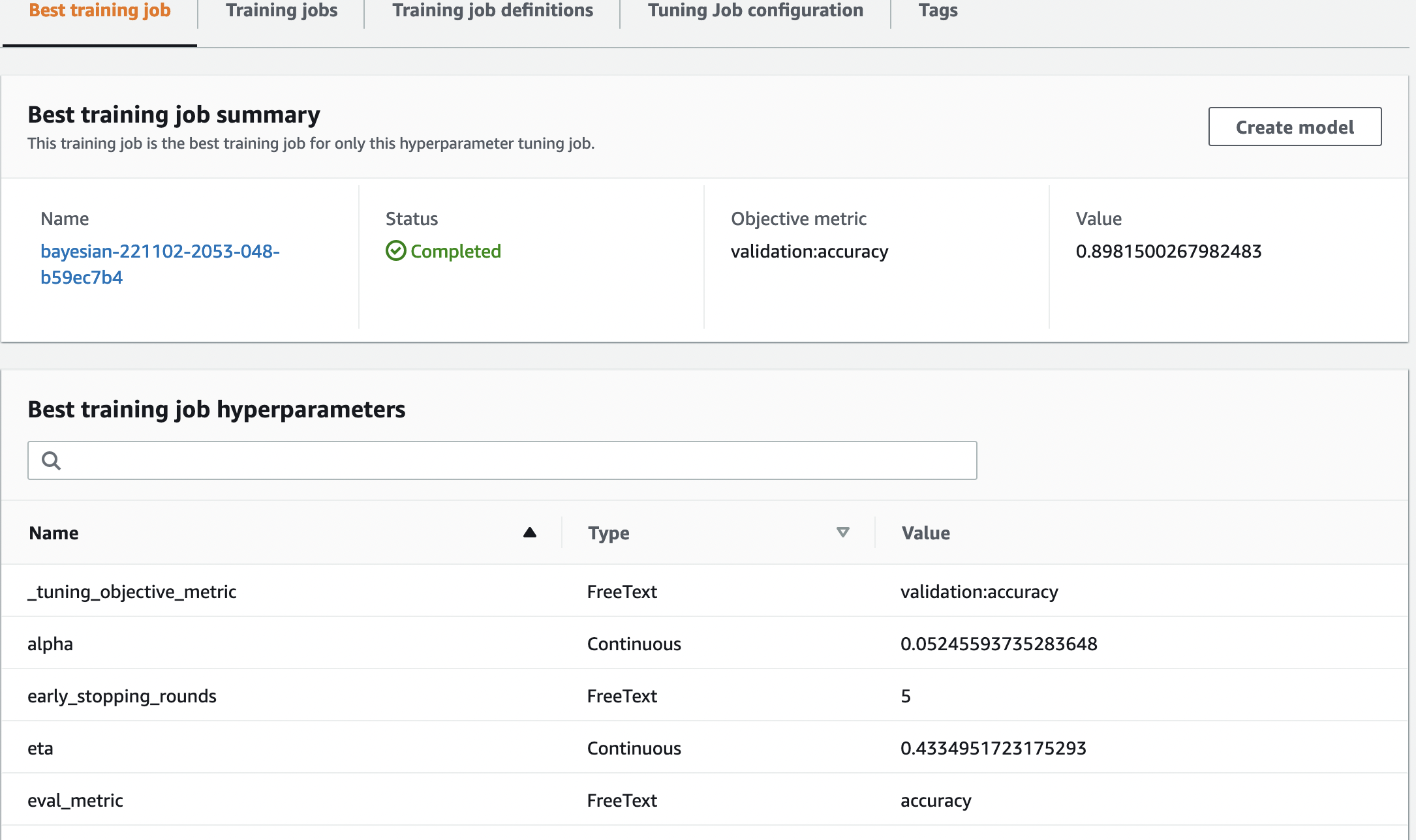
We can immediately see what hyperparameter values led to this superior performance. However, we want to know more. Can you guess what? We see that alpha takes on an approximate value of 0.052456 and, likewise, eta is set to 0.433495. This tells us that these values worked well, but it tells us little about the hyperparameter space itself. For example, we might wonder whether 0.433495 for eta was the highest value tested, or whether there’s room for growth and model improvement by selecting higher values.
For that, we need to zoom out, and take a much wider view to see how other values for our hyperparameters performed. One way to look at a lot of data at once is to plot our hyperparameter values from our HPO trials on a chart. That way we see how these values performed relatively. In the next section, we pull this data from SageMaker and visualize it.
Visualize our trials
The SageMaker SDK provides us with the data for our exploration, and the notebooks give you a peek into that. But there are many ways to utilize and visualize it. In this post, we share a sample using the Altair statistical visualization library, which we use to produce a more visual overview of our trials. These are found in the amtviz package, which we are providing as part of the sample:
from amtviz import visualize_tuning_job
visualize_tuning_job(tuner, trials_only=True)
The power of these visualizations becomes immediately apparent when plotting our trials’ validation accuracy (y-axis) over time (x-axis). The following chart on the left shows validation accuracy over time. We can clearly see the model performance improving as we run more trials over time. This is a direct and expected outcome of running HPO with a Bayesian strategy. In our next post, we see how this compares to other strategies and observe that this doesn’t need to be the case for all strategies.
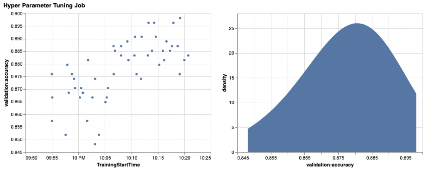
After reviewing the overall progress over time, now let’s look at our hyperparameter space.
The following charts show validation accuracy on the y-axis, with each chart showing max_depth, alpha, eta, and min_child_weight on the x-axis, respectively. We’ve plotted our entire HPO job into each chart. Each point is a single trial, and each chart contains all 50 trials, but separated for each hyperparameter. This means that our best performing trial, #48, is represented by exactly one blue dot in each of these charts (which we have highlighted for you in the following figure). We can visually compare its performance within the context of all other 49 trials. So, let’s look closely.
Fascinating! We see immediately which regions of our defined ranges in our hyperparameter space are most performant! Thinking back to our eta value, it’s clear now that sampling values closer to 0 yielded worse performance, whereas moving closer to our border, 0.5, yields better results. The reverse appears to be true for alpha, and max_depth appears to have a more limited set of preferred values. Looking at max_depth, you can also see how using a Bayesian strategy instructs SageMaker AMT to sample more frequently values it learned worked well in the past.
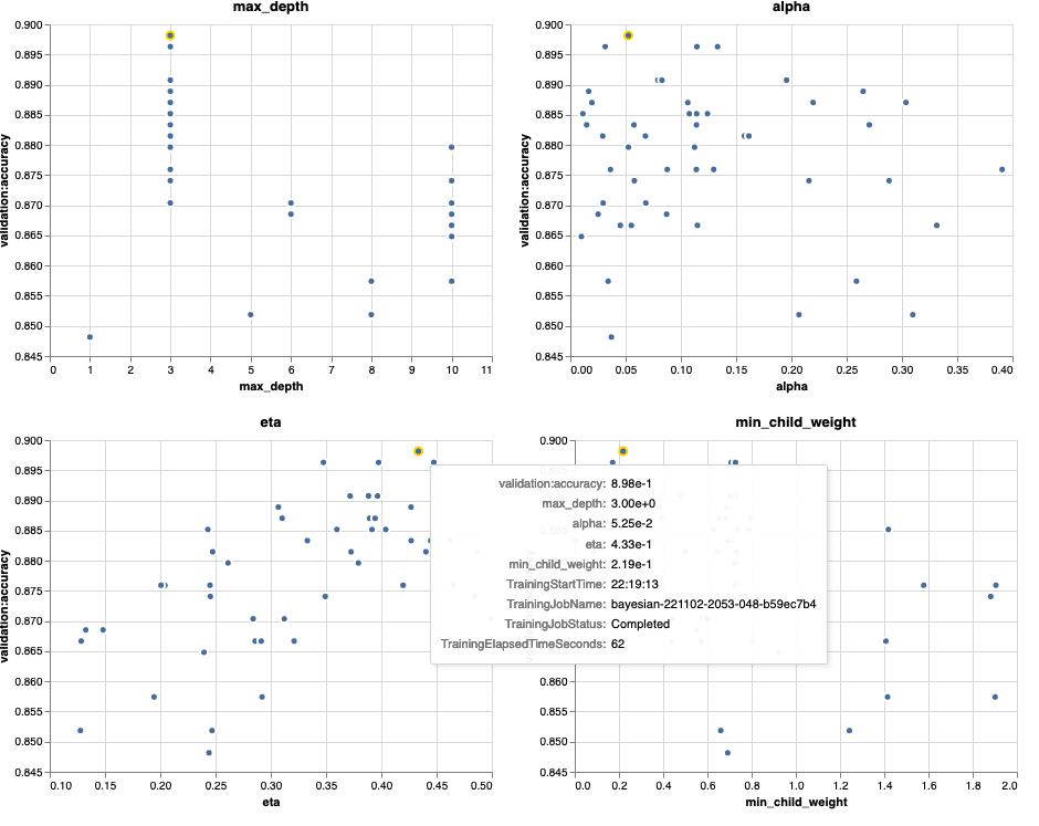
Looking at our eta value, we might wonder whether it’s worth exploring more to the right, perhaps beyond 0.45? Does it continue to trail off to lower accuracy, or do we need more data here? This wondering is part of the purpose of running our first HPO job. It provides us with insights into which areas of the hyperparameter space we should explore further.
If you’re keen to know more, and are as excited as we are by this introduction to the topic, then stay tuned for our next post, where we’ll talk more about the different HPO strategies, compare them against each other, and practice training with our own Python script.
Clean up
To avoid incurring unwanted costs when you’re done experimenting with HPO, you must remove all files in your S3 bucket with the prefix amt-visualize-demo and also shut down Studio resources.
Run the following code in your notebook to remove all S3 files from this post.
!aws s3 rm s3://{BUCKET}/amt-visualize-demo --recursive
If you wish to keep the datasets or the model artifacts, you may modify the prefix in the code to amt-visualize-demo/data to only delete the data or amt-visualize-demo/output to only delete the model artifacts.
Conclusion
In this post, we trained and tuned a model using the SageMaker built-in version of the XGBoost algorithm. By using HPO with SageMaker AMT, we learned about the hyperparameters that work well for this particular algorithm and dataset.
We saw several ways to review the outcomes of our hyperparameter tuning job. Starting with extracting the hyperparameters of the best trial, we also learned how to gain a deeper understanding of how our trials had progressed over time and what hyperparameter values are impactful.
Using the SageMaker console, we also saw how to dive deeper into individual training runs and review their logs.
We then zoomed out to view all our trials together, and review their performance in relation to other trials and hyperparameters.
We learned that based on the observations from each trial, we were able to navigate the hyperparameter space to see that tiny changes to our hyperparameter values can have a huge impact on our model performance. With SageMaker AMT, we can run hyperparameter optimization to find good hyperparameter values efficiently and maximize model performance.
In the future, we’ll look into different HPO strategies offered by SageMaker AMT and how to use our own custom training code. Let us know in the comments if you have a question or want to suggest an area that we should cover in upcoming posts.
Until then, we wish you and your models happy learning and tuning!
References
Citations:
[1] Dua, D. and Graff, C. (2019). UCI Machine Learning Repository [http://archive.ics.uci.edu/ml]. Irvine, CA: University of California, School of Information and Computer Science.
About the authors
 Andrew Ellul is a Solutions Architect with Amazon Web Services. He works with small and medium-sized businesses in Germany. Outside of work, Andrew enjoys exploring nature on foot or by bike.
 Elina Lesyk is a Solutions Architect located in Munich. Her focus is on enterprise customers from the Financial Services Industry. In her free time, Elina likes learning guitar theory in Spanish to cross-learn and going for a run.
 Mariano Kamp is a Principal Solutions Architect with Amazon Web Services. He works with financial services customers in Germany on machine learning. In his spare time, Mariano enjoys hiking with his wife.
Read More


 Our partnership with iCAD Inc. marks the first time we are licensing our mammography AI model in clinical practice.
 Vikas Shah is an Enterprise Solutions Architect at Amazon web services. He is a technology enthusiast who enjoys helping customers find innovative solutions to complex business challenges. His areas of interest are ML, IoT, robotics and storage. In his spare time, Vikas enjoys building robots, hiking, and traveling.


 Bharadwaj Tanikella is a Senior Product Manager for Amazon CodeWhisperer. He has a background in Machine Learning, both as a developer and a Product Manager. In his spare time he loves to bike, read non-fiction and learning new languages.