Monthly Archives: November 2022

Amazon Rekognition is a computer vision service that makes it simple to add image and video analysis to your applications using proven, highly scalable, deep learning technology that does not require machine learning (ML) expertise. With Amazon Rekognition, you can identify objects, people, text, scenes, and activities in images and videos and detect inappropriate content. Amazon Rekognition also provides highly accurate facial analysis and facial search capabilities that you can use to detect, analyze, and compare faces for a wide variety of use cases.

Amazon Rekognition Custom Labels is a feature of Amazon Rekognition that makes it simple to build your own specialized ML-based image analysis capabilities to detect unique objects and scenes integral to your specific use case.

Some common use cases of Rekognition Custom Labels include finding your logo in social media posts, identifying your products on store shelves, classifying machine parts in an assembly line, distinguishing between healthy and infected plants, and more.

Amazon Rekognition Labels supports popular landmarks like the Brooklyn Bridge, Colosseum, Eiffel Tower, Machu Picchu, Taj Mahal, and more. If you have other landmarks or buildings not yet supported by Amazon Rekognition, you can still use Amazon Rekognition Custom Labels.

In this post, we demonstrate using Rekognition Custom Labels to detect the Amazon Spheres building in Seattle.

With Rekognition Custom Labels, AWS takes care of the heavy lifting for you. Rekognition Custom Labels builds off the existing capabilities of Amazon Rekognition, which is already trained on tens of millions of images across many categories. Instead of thousands of images, you simply need to upload a small set of training images (typically a few hundred images or less) that are specific to your use case via our straightforward console. Amazon Rekognition can begin training in just a few clicks. After Amazon Rekognition begins training from your image set, it can produce a custom image analysis model for you within few minutes or hours. Behind the scenes, Rekognition Custom Labels automatically loads and inspects the training data, selects the suitable ML algorithms, trains a model, and provides model performance metrics. You can then use your custom model via the Rekognition Custom Labels API and integrate it into your applications.

Solution overview

For our example, we use the Amazon Spheres building in Seattle. We train a model using Rekognition Custom Labels; whenever similar images are used, the algorithm should identify it as Amazon Spheres instead of Dome, Architecture, Glass building, or other labels.

Let’s first show an example of using the label detection feature of Amazon Rekognition, where we feed the image of Amazon Spheres without any custom training. We use the Amazon Rekognition console to open the label detection demo and upload our photo.

After the image is uploaded and analyzed, we see labels with their confidence scores under Results. In this case, Dome was detected with confidence score of 99.2%, Architecture with 99.2%, Building with 99.2%, Metropolis with 79.4%, and so on.

We want to use custom labeling to produce a computer vision model that can label the image Amazon Spheres.

In the following sections, we walk you through preparing your dataset, creating a Rekognition Custom Labels project, training the model, evaluating the results, and testing it with additional images.

Prerequisites

Before starting with the steps, there are quotas for Rekognition Custom Labels that you need to be aware of. If you want to change the limits, you can request a service limit increase.

Create your dataset

If this is your first time using Rekognition Custom Labels, you’ll be prompted to create an Amazon Simple Storage Service (Amazon S3) bucket to store your dataset.

For this blog demonstration, we have used images of the Amazon Spheres, which we captured while we visited Seattle, WA. Feel free to use your own images as per your need.

Copy your dataset to the newly created bucket, which stores your images inside their respective prefixes.

Create a project

To create your Rekognition Custom Labels project, complete the following steps:

1. On the Rekognition Custom Labels console, choose Create a project.
2. For Project name, enter a name.
3. Choose Create project.
   
   Now we specify the configuration and path of your training and test dataset.
4. Choose Create dataset.
   

You can start with a project that has a single dataset, or a project that has separate training and test datasets. If you start with a single dataset, Rekognition Custom Labels splits your dataset during training to create a training dataset (80%) and a test dataset (20%) for your project.

Additionally, you can create training and test datasets for a project by importing images from one of the following locations:

• An S3 bucket
• A local computer
• Amazon SageMaker Ground Truth
• An existing dataset

For this post, we use our own custom dataset of Amazon Spheres.

1. Select Start with a single dataset.
2. Select Import images from S3 bucket.
   
3. For S3 URI, enter the path to your S3 bucket.
4. If you want Rekognition Custom Labels to automatically label the images for you based on the folder names in your S3 bucket, select Automatically assign image-level labels to images based on the folder name.
   
5. Choose Create dataset.

A page opens that shows you the images with their labels. If you see any errors in the labels, refer to Debugging datasets.

Train the model

After you have reviewed your dataset, you can now train the model.

1. Choose train model.
2. For Choose project, enter the ARN for your project if it’s not already listed.
3. Choose Train model.

In the Models section of the project page, you can check the current status in the Model status column, where the training is in progress. Training time typically takes 30 minutes to 24 hours to complete, depending on several factors such as number of images and number of labels in the training set, and types of ML algorithms used to train your model.

When the model training is complete, you can see the model status as TRAINING_COMPLETED. If the training fails, refer to Debugging a failed model training.

Evaluate the model

Open the model details page. The Evaluation tab shows metrics for each label, and the average metric for the entire test dataset.

The Rekognition Custom Labels console provides the following metrics as a summary of the training results and as metrics for each label:

• Precision
• Recall
• F1

You can view the results of your trained model for individual images, as shown in the following screenshot.

Test the model

Now that we’ve viewed the evaluation results, we’re ready to start the model and analyze new images.

You can start the model on the Use model tab on the Rekognition Custom Labels console, or by using the StartProjectVersion operation via the AWS Command Line Interface (AWS CLI) or Python SDK.

When the model is running, we can analyze the new images using the DetectCustomLabels API. The result from DetectCustomLabels is a prediction that the image contains specific objects, scenes, or concepts. See the following code:

aws rekognition detect-custom-labels 
--project-version-arn <value> 
--image '{"S3Object": {"Bucket":<"MY_BUCKET">,"Name":<"PATH_TO_MY_IMAGE">}}' 
--region <value>

In the output, you can see the label with its confidence score:

{
    "Custom Labels": [
        {
            "Name": "Amazon Spheres",
            "Confidence": 93.55500030517578
        }
    ]
}

As you can see from the result, just with few simple clicks, you can use Rekognition Custom Labels to achieve accurate labeling outcomes. You can use this for a multitude of image use cases, such as identifying custom labeling for food products, pets, machine parts, and more.

Clean up

To clean up the resources you created as part of this post and avoid any potential recurring costs, complete the following steps:

1. On the Use model tab, stop the model.
   Alternatively, you can stop the model using the StopProjectVersion operation via the AWS CLI or Python SDK.Wait until the model is in the Stopped state before continuing to the next steps.
2. Delete the model.
3. Delete the project.
4. Delete the dataset.
5. Empty the S3 bucket contents and delete the bucket.

Conclusion

In this post, we showed how to use Rekognition Custom Labels to detect building images.

You can get started with your custom image datasets, and with a few simple clicks on the Rekognition Custom Labels console, you can train your model and detect objects in images. Rekognition Custom Labels can automatically load and inspect the data, select the right ML algorithms, train a model, and provide model performance metrics. You can review detailed performance metrics such as precision, recall, F1 scores, and confidence scores.

The day has come when we can now identify popular buildings like Empire State Building in New York City, the Taj Mahal in India, and many others across the world pre-labeled and ready to use for intelligence in your applications. But if you have other landmarks currently not yet supported by Amazon Rekognition Labels, look no further and try out Amazon Rekognition Custom Labels.

For more information about using custom labels, see What Is Amazon Rekognition Custom Labels? Also, visit our GitHub repo for an end-to-end workflow of Amazon Rekognition custom brand detection.

About the Authors:

Suresh Patnam is a Principal BDM – GTM AI/ML Leader at AWS. He works with customers to build IT strategy, making digital transformation through the cloud more accessible by leveraging Data & AI/ML. In his spare time, Suresh enjoys playing tennis and spending time with his family.

Bunny Kaushik is a Solutions Architect at AWS. He is passionate about building AI/ML solutions on AWS and helping customers innovate on the AWS platform. Outside of work, he enjoys hiking, climbing, and swimming.

Read More

Amazon Forecast is a fully managed service that uses statistical and machine learning (ML) algorithms to deliver highly accurate time-series forecasts. Recently, based on Amazon Forecast, we helped one of our retail customers achieve accurate demand forecasting, within 8 weeks. The solution improved the manual forecast by an average of 10% in regards to the WAPE metric. This leads to a direct savings of 16 labor hours monthly. In addition, we estimated that by fulfilling the correct number of items, sales could increase by up to 11.8%. In this post, we present the workflow and the critical elements to implement—from proof of concept (POC) to production—a demand forecasting system with Amazon Forecast, focused on challenges in the retail industry.

Background and current challenges of demand forecasting in the retail industry

The goal of demand forecasting is to estimate future demand from historical data, and to help store replenishment and capacity allocation. With demand forecasting, retailers are able to position the right amount of inventory at each location in their network to meet demand. Therefore, an accurate forecasting system can drive a wide range of benefits across different business functions, such as:

• Increasing sales from better product availability and reducing the effort of inter-store transfer waste
• Providing more reliable insight to improve capacity utilization and proactively avoid bottlenecks in capacity provisioning
• Minimizing inventory and production costs and improve inventory turnover
• Presenting an overall better customer experience

ML techniques demonstrate great value when a large volume of good quality data is present. Today, experience-based replenishment management or demand forecast is still the mainstream for most retailers. With the goal to improve the customer experience, more and more retailers are willing to replace experience-based demand forecasting systems with ML-based forecasts. However, retailers face multiple challenges when implementing ML-based demand forecasting systems into production. We summarize the different challenges into three categories: data challenges, ML challenges, and operational challenges.

Data challenges

A large volume of clean, quality data is a key requirement for driving accurate ML-based predictions. Quality data, including historical sales and sales-related data (such as inventory, item pricing, and promotions), needs to be collected and consolidated. The diversity of data from multiple resources requires a modern data platform to unite data silos. In addition, access to data in a timely manner is necessary for frequent and fine-grained demand forecasts.

ML challenges

Developing advanced ML algorithms requires expertise. Implementing the right algorithms for the right problem needs both in-depth domain knowledge and ML competences. In addition, learning from large available datasets requires a scalable ML infrastructure. Moreover, maintaining ML algorithms in production requires ML competences in order to analyze the root cause of model degradation and correctly retrain the model.

To solve practical business problems, producing accurate forecasts is only part of the story. Decision-makers need probabilistic forecasts at different quantiles make important customer experience vs. financial results trade-off decisions. They also need to explain predictions to stakeholders, and perform what-if analyses to investigate how different scenarios might affect forecast results.

Operational challenges

Reducing the operational effort of maintaining a cost-effective forecasting system is the third principal challenge. In a common scenario of demand forecasting, each item at each location has its own forecast. A system that can manage hundreds of thousands of forecasts at any time is required. In addition, business end-users need the forecasting system to be integrated into existing downstream systems, such as existing supply chain management platforms, so that they can use ML-based systems without modifying existing tools and processes.

These challenges are especially acute when business are large, dynamic, and growing. To address these challenges, we share a customer success story that reduces the efforts to quickly validate the potential business gain. This is achieved through prototyping with Amazon Forecast—a fully managed service that provides accurate forecasting results without the need to manage underlying infrastructure resources and algorithms.

Rapid prototyping for an ML-based forecasting system with Amazon Forecast

Based on our experience, we often see that retail customers are willing to initiate a proof of concept on their sales data. This can be done within a range of a few days to a few weeks for rapid prototyping, depending on the data complexity and available resources to iterate through the model tuning process. During prototyping, we suggest using sprints to effectively manage the process, and separating the POC into data exploration, iterative improvement, and automation phases.

Data exploration

Data exploration often involves intense discussion with data scientists or business intelligence analysts to get familiar with the historical sales dataset and available data sources that can potentially impact forecast results, such as inventory and historical promotional events. One of the most efficient ways is to consolidate the sales data, as the target dataset, from the data warehouse at the early stage of the project. This is based on the fact that forecast results are often dominated by the target dataset patterns. Data warehouses often store day-to-day business data, and an exhaustive understanding within a short period of time is difficult and time consuming. Our suggestion is to concentrate on generating the target dataset and make sure this dataset is correct. These data exploration and baseline results can often be achieved within a few days, and this can determine if the target data can be accurately forecasted. We discuss data forecastability later in this post.

Iteration

After we have the baseline results, we can continue adding more related data to see how these can impact accuracy. This is often done through a deep dive into additional datasets; for more information, refer to Using Related Time Series Datasets and Using Item Metadata Datasets.

In some cases, it may be possible to improve accuracy in Amazon Forecast by training the models with similarly behaving subsets of the dataset, or by removing the sparse data from the dataset. During this iterative improvement phase, the challenging part—true for all ML projects—is that the current iteration depends on the previous iteration’s key findings and insights, so rigorous analysis and reporting is key for success.

Analysis can be done quantitatively and empirically. The quantitative aspect refers to evaluation during the backtesting and comparing the accuracy metric, such as WAPE. The empirical aspect refers to visualizing the prediction curve and actual target data, and using the domain knowledge to incorporate potential factors. These analyses help you iterate faster to bridge the gap between forecasted results and target data. In addition, presenting such results via a weekly report can often provide confidence to business end-users.

Automation

The final step often involves the discussion of POC to production procedure and automation. Because the ML project is constrained by the total project duration, we might not have enough time to explore every possibility. Therefore, indicating the potential area throughout the findings during the project can often earn trust. In addition, automation can help business end-users evaluate Forecast for a longer period, because they can use an existing predictor to generate forecasts with the updated data.

The success criteria can be evaluated with generated results, both from technical and business perspectives. During the evaluation period, we can estimate potential benefits for the following:

• Increasing the forecast accuracy (technical) – Compute the prediction accuracy with regards to actual sales data, and compare with the existing forecast system, including manual forecasts
• Reducing waste (business) – Reduce over-forecasting in order to reduce waste
• Improving in-stock rates (business) – Reduce under-forecasting in order to improve in-stock rates
• Estimating the increase of gross profit (business) – Reduce wastage and improve in-stock rates in order to increase gross profit

We summarize the development workflow in the following diagram.

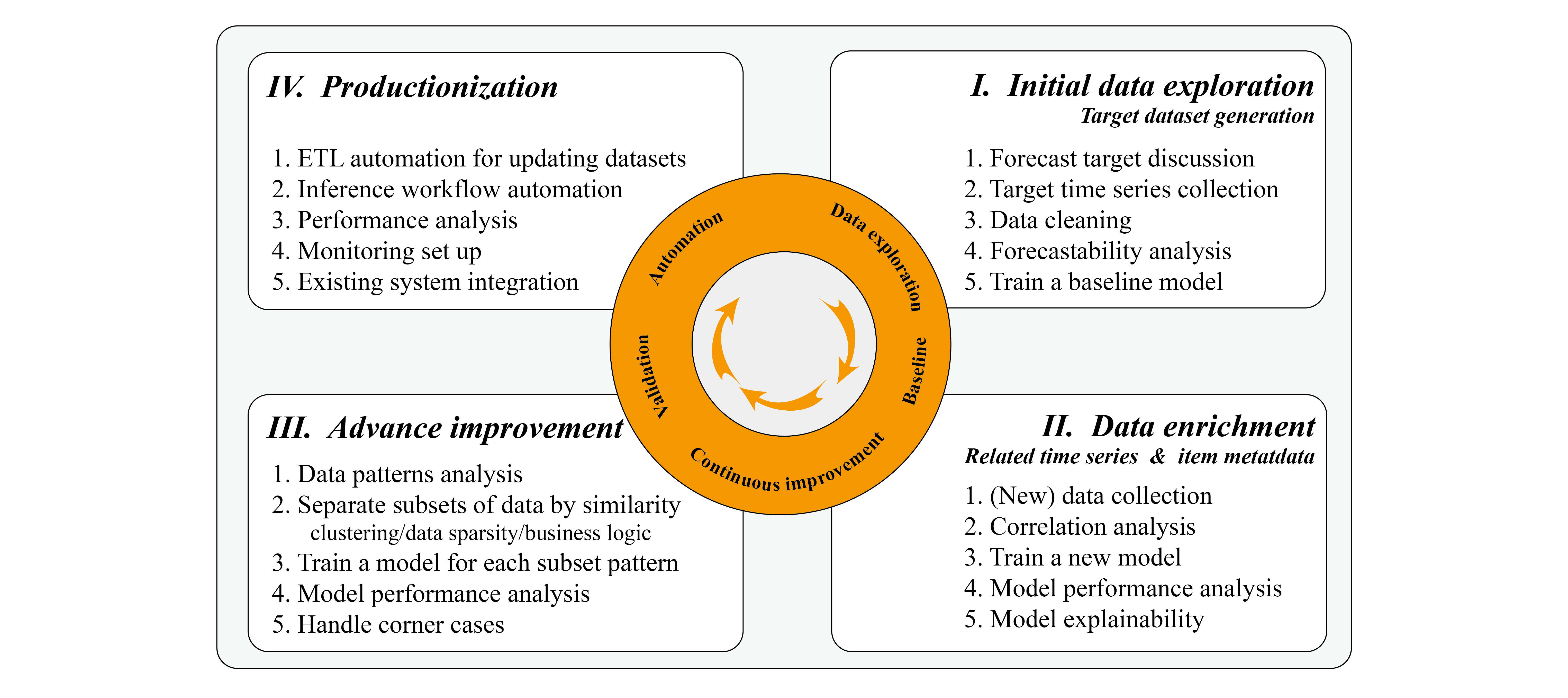
In the following sections, we discuss the important elements to take into consideration during the implementation.

Step-by-step workflow for developing a forecasting system

Target dataset generation

The first step is to generate the target dataset for Forecast. In the retail industry, this refers to the historical time series demand and sales data for retail items (SKUs). When preparing the dataset, one important aspect is granularity. We should consider the data granularity from both business requirements and technical requirements.

The business defines how forecasting results in the production system:

• Horizon – The number of time steps being forecasted. This depends on the underlying business problem. If we want to refill the stock level each week, then a weekly forecast or daily forecast seems appropriate.
• Granularity – The granularity of your forecasts: time frequency such as daily or weekly, different store locations, and different sizes of the same item. In the end, the prediction can be a combination of each store SKU, with daily data points.

Although the aforementioned forecast horizon and granularity should be defined to prioritize the business requirement, we might need to make trade-offs between requirements and feasibility. Take the footwear business as one example. If we want to predict sales of each shoe size at each store level, the data soon becomes sparse and the pattern is hard to find. However, to refill stock, we need to estimate this granularity. To do this, alternative solutions might require estimating a ratio between different shoe sizes and using this ratio to calculate fine-grained results.

We often need to balance the business requirement and the data pattern that can be learned and used for forecasting. To provide a quantitative qualification of the data patterns, we propose using data forecastability.

Data forecastability and data pattern classification

One of the key insights that we can collect from the target dataset is its ability to produce quality forecasts. This can be analyzed at the very early phase of the ML project. Forecast shines when data shows seasonality, trends, and cyclical patterns.

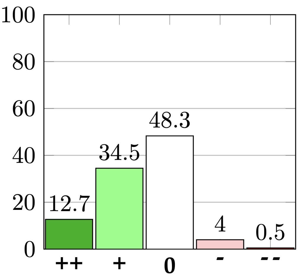
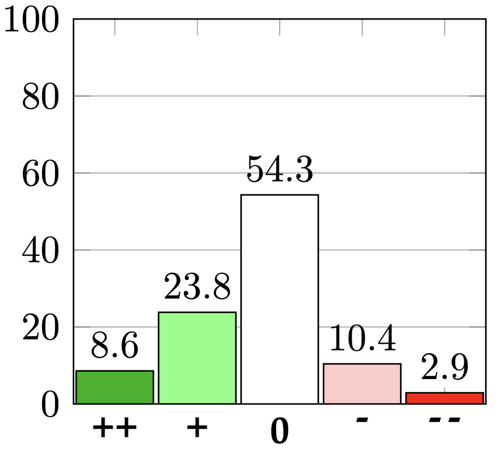
To determine forecastability, there are two major coefficients: variability in demand timing and variability in demand quantity. Variability in demand timing means the interval between two instances of demand, and it measures the demand regularity in time. Variability in demand quantity means variation in quantities. The following figure illustrates some different patterns. Forecast accuracy strongly depends on product forecastability. For more information, refer to Demand classification: why forecastability matters.

It’s worth noting that this forecastability analysis is for each fine-grained item (for example, SKU-Store-Color-Size). It’s quite common that in a demand forecasting production system, different items follow different patterns. Therefore, it’s important to separate the items following different data patterns. One typical example is fast-moving and slow-moving items; another example would be dense and sparse data. In addition, a fine-grained item has more chances of yielding a lumpy pattern. For example, in a clothing store, the sales of one popular item can be quite smooth daily, but if we further separate the sales of the item for each color and size, it soon becomes sparse. Therefore, reducing the granularity from SKU-Store-Color-Size to SKU-Store can change the data pattern from lumpy to smooth, and vice versa.

Moreover, not all items contribute to sales equally. We have observed that item contribution often follows the Pareto distribution, in which top items contribute most of the sales. The sales of these top items are often smooth. Items with a lower sales record are often lumpy and erratic, and therefore hard to estimate. Adding these items might actually decrease the accuracy of top sales items. Based on these observations, we can separate the items into different groups, train the Forecast model on top sales items, and handle the lower sales items as corner cases.

Data enrichment and additional dataset selection

When we want to use additional datasets to improve the performance of forecast results, we can rely on time series datasets and metadata datasets. In the retail domain, based on intuition and domain knowledge, features such as inventory, price, promotion, and winter or summer seasons could be imported as the related time series. The simplest way to identify usefulness of features is via feature importance. In Forecast, this is done by explainability analysis. Forecast Predictor Explainability helps us better understand how the attributes in the datasets impact forecasts for the target. Forecast uses a metric called impact scores to quantify the relative impact of each attribute and determine whether they increase or decrease forecast values. If one or more attributes have an impact score of zero, then these attributes have no significant impact on forecast values. This way, we can quickly remove the features that have less impact and add the potential ones iteratively. It’s important to note that impact scores measure the relative impact of attributes, which are normalized together with impact scores of all other attributes.

Like all ML projects, improving accuracy with additional features requires iterative experiments. You need to experiment with multiple combinations of datasets, while observing the impact of incremental changes on model accuracy. You can try to run multiple Forecast experiments via the Forecast console or with Python notebooks with Forecast APIs. In addition, you can onboard with AWS CloudFormation, which deploys AWS provided ready-made solutions for common use cases (for example, the Improving Forecast Accuracy with Machine Learning solution). Forecast automatically separates the dataset and produces accuracy metrics to evaluate predictors. For more information, see Evaluating Predictor Accuracy. This helps data scientists iterate faster to achieve the best performing model.

Advanced improvement and handling corner cases

We mentioned that forecast algorithms can learn seasonality, trends, and cyclical features from data. For items with these characteristics, and the appropriate data density and volume, we can use Forecast to generate estimations. However, when facing lumpy data patterns, especially when the data volume is small, we might need to handle them differently, such as with empirical estimation based on a ruleset.

For dense SKUs, we further improve Forecast accuracy by training the models with similarly behaving subsets of the time series dataset. The subset separation strategies that we used are business logic, product type, data density, and patterns learned by the algorithm. After the subsets are generated, we can train multiple Forecast models for the different subsets. For one such example, refer to Cluster time series data for use with Amazon Forecast.

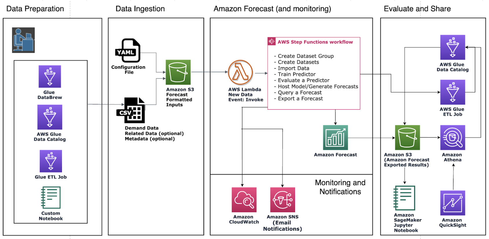
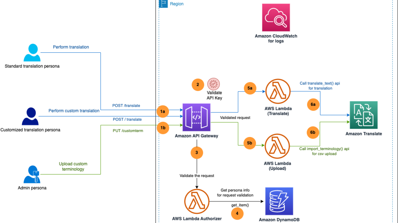
Toward production: Updating the dataset, monitoring, and retraining

Let’s explore an example architecture with Forecast, as shown in the following diagram. Each time an end-user consolidates a new dataset on Amazon Simple Storage Service (Amazon S3), it triggers AWS Step Functions to orchestrate different components, including creating the dataset import job, creating an auto predictor, and generating forecasts. After the forecast results are generated, the Create Forecast Export step exports them to Amazon S3 for downstream consumers. For more information about how to provision this automated pipeline, refer to Automating with AWS CloudFormation. It uses a CloudFormation stack to automatically deploy datasets to an S3 bucket and trigger a Forecast pipeline. You can use the same automation stack to generate forecasts with your own datasets.

There are two ways to incorporate recent trends into the forecasting system: updating data or retraining the predictor.

To generate the forecast with updated data reflecting recent trends, you need to upload the updated input data file to an S3 bucket (the updated input data should still contain all of your existing data). Forecast doesn’t automatically retrain a predictor when you import an updated dataset. You can generate forecasts as you usually do. Forecast predicts the forecast horizon starting from the last day in the updated input data. Therefore, recent trends are incorporated into any new inferences produced by Forecast.

However, if you want your predictor to be trained off of the new data, you must create a new predictor. You might need to consider retraining the model when data patterns (seasonality, trends, or cycles) change. As mentioned in Continuously monitor predictor accuracy with Amazon Forecast, the performance of a predictor will fluctuate over time, due to factors such as changes in the economic environment or in consumer behavior. Therefore, the predictor may need to be retrained, or a new predictor may need to be created to ensure highly accurate predictions continue to be made. With the help of predictor monitoring, Forecast can track the quality of your predictors, allowing you to reduce operational efforts, while helping you make more informed decisions about keeping, retraining, or rebuilding your predictors.

Conclusion

Amazon Forecast is a time series forecasting service based on ML and built for business metrics analysis. We can integrate demand forecasting prediction with high accuracy by combining historical sales and other relevant information such as inventory, promotions, or season. Within 8 weeks, we helped one of our retail customers achieve accurate demand forecasting—10% improvement in comparison with the manual forecast. This leads to a direct savings of 16 labor hours monthly and estimated sales increase by up to 11.8%.

This post shared common practices for bringing your forecasting project from proof of concept to production. Get started now with Amazon Forecast to achieve highly accurate forecasts for your business.

About the Authors

Yanwei Cui, PhD, is a Machine Learning Specialist Solutions Architect at AWS. He started machine learning research at IRISA (Research Institute of Computer Science and Random Systems), and has several years of experience building artificial intelligence powered industrial applications in computer vision, natural language processing and online user behavior prediction. At AWS, he shares the domain expertise and helps customers to unlock business potentials, and to drive actionable outcomes with machine learning at scale. Outside of work, he enjoys reading and traveling.

Gordon Wang is a Senior Data Scientist on the Professional Services team at Amazon Web Services. He supports customers in many industries, including media, manufacturing, energy, retail, and healthcare. He is passionate about computer vision, deep learning, and MLOps. In his spare time, he loves running and hiking.

Read More

Enterprises often need to communicate effectively to a large base of customers, partners, and stakeholders across several different languages. They need to translate and localize content such as marketing materials, product content assets, operational manuals, and legal documents. Each business unit in the enterprise has different translation workloads and often manages their own translation requirements and vendors. While this distributed approach may give business units translation autonomy and flexibility, it becomes difficult for enterprises to maintain translation consistency across the enterprise.

Amazon Translate is a neural machine translation service that delivers fast, high-quality, affordable, and customizable language translation. Today, Amazon Translate supports scalable language translation for over 5,500 language pairings in batch and real time. It can be used to build solutions that address the challenge enterprises with multiple business units face when looking for ways to accelerate multilingual workflows with customization support.

For example, the BMW Group needed a unified translation solution to help their business units, such as Sales and Manufacturing, use translation technology at scale and remove common mistranslation issues across the enterprise. Their solution with Amazon Translate reduces translation time by over 75% while simultaneously giving each business unit the ability to customize the output to address their specific translation requirements.

In this blog post, we demonstrate how to build a unified translation solution with customization features using Amazon Translate and other AWS services. We’ll also show you how to install and test the solution and how you can build a customizable and scalable translation solution for users depending on their department’s localization needs.

Solution overview

The solution uses Amazon Translate’s native features such as real-time translation, automatic source language detection, and custom terminology. Using Amazon API Gateway, these features are exposed as one simple /translate API. Custom terminology allows you to define specific custom translation pairs. In order for custom terminology to work, you need to upload a terminology file to Amazon Translate. Therefore, another API /customterm is exposed.

The solution illustrates two options for translation: a standard translation and a customized translation (using the custom terminology feature). However, you can modify these options as needed to suit your business requirements. Consumers can use these options using API Gateway’s API keys. When a translation request is received by the API, it validates the request (using an AWS Lambda authorizer function) whether the provided API key is authorized to perform the type of translation requested. We use an Amazon DynamoDB table to store metadata information about consumers, permissions, and API keys.

This solution caters to three persona types:

• Standard translation persona – Users within a business unit having no customization requirements. This includes standard translation options and features such as automatic language detection of Amazon Translate.
• Customized translation persona – Users within a business unit having customization requirements. This includes all the features for standard translation as well as the ability to customize the translations using a custom terminology file.
• Admin persona – Supports the customized translation option by managing the uploading of custom terminology files but is not able to make any other translation API calls.

The following diagram illustrates the centralized translation solution with customization architecture.

For the user translation persona, the process includes the following actions (the blue path in the preceding diagram):

1a. Call the /translate API and pass the API key in the API header. Optionally, for the customized translation persona, the user can enable custom translation by passing in an optional query string parameter (useCustomTerm).

2. API Gateway validates the API key.

3. The Lambda custom authorizer is called to validate the action that the supplied API key is allowed. For instance, a standard translation persona can’t ask for custom translation, or an administrator can’t perform any text translation.

4. The Lambda authorizer gets the user information from the DynamoDB table and verifies against the API key provided.

5a. After validation, another Lambda function (Translate) is invoked to call the Amazon Translate API translate_text.

6a. The translated text is returned in the API response.

The admin persona can upload a custom terminology file that can be used by the customized translation persona by calling the /customterm API. The workflow steps are follows (the green path in the preceding diagram):

1b. Call the /customterm API and pass the API key in the API header.

2. API Gateway validates the API key.

3. The Lambda custom authorizer is called to validate the action that the supplied API key is allowed. For instance, only an admin persona can upload custom terminology files.

4. The Lambda authorizer gets the user information from the DynamoDB table and verifies against the API key provided.

5b. After the API key is validated, another Lambda function (Upload) is invoked to call the Amazon Translate API import_terminology.

6b. The custom terminology file is uploaded to Amazon Translate with a unique name generated by the Lambda function.

In the following sections, we walk through the steps to deploy and test the solution.

Prerequisites

To deploy the solution, you need an AWS account. If you don’t already have an AWS account, you can create one. Your access to the AWS account must have AWS Identity and Access Management (IAM) permissions to launch AWS CloudFormation templates that create IAM roles.

Note that you are responsible for the cost of the AWS services used while running this sample deployment. Many of these services (such as Amazon Translate, API Gateway, and Lambda) come with a Free Tier to get you started. For full details, see the pricing pages for each AWS service that you use in this post.

Deploy the solution with AWS CloudFormation

Launch the provided CloudFormation template to deploy the solution in your AWS account. This stack only works in the us-east-1 or eu-west-1 Regions. If you want to deploy this solution in other Regions, refer to the GitHub repo and deploy the CloudFormation in your Region of choice.

1. Deploy the latest CloudFormation template by following the link for your preferred Region:

Region	CloudFormation Stack
N. Virginia (us-east-1)
Ireland (eu-west-1)

2. If prompted, log in using your AWS account credentials.
3. Leave the fields on the Create stack page with their pre-populated defaults.
4. Choose Next.
5. For Stack name, enter the name of the CloudFormation stack (for this post, EnterpriseTranslate).
6. For DDBTableName¸ enter the name of the DynamoDB table (EnterpriseTranslateTable).
7. For apiGatewayName, enter the API Gateway created by the stack (EnterpriseTranslateAPI).
8. For apiGatewayStageName, enter the environment name for API Gateway (prod).
9. Choose Next.
10. On the review page, select the check boxes to acknowledge the creation of IAM resources.This is required to allow CloudFormation to create a role to grant access to the resources needed by the stack and name the resources in a dynamic way.
11. Choose Create stack.

You can monitor the stack creation progress on the Events tab. The stack is complete when the stack status shows as CREATE_COMPLETE.

The deployment creates the following resources (all prefixed with EntTranslate):

• An API Gateway API with two resources called /customterm and /translate, with three API keys to represent two translation personas and an admin persona
• A DynamoDB table with three items to reflect one consumer with three different roles (three API keys)
• Several Lambda functions (using Python 3.9) as per the architecture diagram

After the resources are deployed into your account on the AWS Cloud, you can test the solution.

Collect API keys

Complete the following steps to collect the API keys:

1. Navigate to the Outputs tab of the CloudFormation stack and copy the value of the key apiGatewayInvokeURL.To find the API keys created by the solution, look in the DynamoDB table you just created or navigate to the API keys page on the API Gateway console. This post uses the latter approach.
2. On the Resources tab of the CloudFormation stack, find the logical ID EntTranslateApi for API Gateway and open the link under the Physical ID column in a new tab.
3. On the API Gateway console, choose API Keys in the navigation pane.
4. Note the three API keys (standard, customized, admin) generated by the solution. For example, select standard key EntTranslateCus1StandardTierKey and choose Show link against the API key property.

Now you can test the APIs using any open-source tools of your choosing. For this post, we use the Postman API testing tool for illustration purposes only. For details on testing API with Postman, refer to API development overview.

Test 1: Standard translation

To test the standard translation API, you first create a POST request in Postman.

1. Choose Add Request in Postman.
2. Set the method type as POST.
3. Enter the API Gateway invoke URL from Output tab of deployed CloudFormation stack.
4. Add /translate to the URL endpoint.
5. On the Headers tab, add a new header key named x-api-key.
6. Enter the standard API key value (copied in Collect API keys stage).
7. On the Body tab, select Raw and enter a JSON body as follows:

   {   "sourceText": "some text to translate",   "targetLanguage": "fr",   "sourceLanguage":"en"}

   sourceLanguage is an optional parameter. If you don’t provide it, the system will set it as auto for the automatic detection of the source language.

8. Call the API by choosing Send and verify the output.
   

The API should run successfully and return the translated text in the Body section of the response object.

Test 2: Customized translation with custom terminology

To test the custom term upload functionality, we first create a PUT request in Postman.

1. Choose Add Request in Postman.
2. Set the method type as PUT.
3. Enter the API Gateway invoke URL.
4. Add /customterm to the end of the URL.
5. On the Headers tab, add a new header key named x-api-key.
6. Enter the admin API key value (copied in Collect API keys stage).
7. On the Body tab, change the format to binary and upload the custom term CSV file. A sample CSV file is provided under the /Resources folder in GitHub repo.
8. Call the API by choosing Send and verify the output.
   
   The API should run successfully with a message in the Body section of the response object saying “Custom term uploaded successfully”
9. On the Amazon Translate console, choose Custom Terminology in the navigation pane.
   A custom terminology file should have been uploaded and is displayed in the terminology list. The file name syntax is the customer ID from the DynamoDB table for the selected API key followed by string _customterm_1.
   Note that if you didn’t use the admin API key, the system will fail to upload the custom term file.Now you’re ready to perform your custom translation.
10. Choose Add Request in Postman.
11. Set the method type as POST.
12. Enter the API Gateway invoke URL.
13. Add /translate to the URL endpoint.
14. On the Headers tab, add a new header key named x-api-key.
15. Enter the standard API key value.
16. On the Body tab, enter a JSON body as follows:

    {   "sourceText": "some text to translate",   "targetLanguage": "fr",   "sourceLanguage":"en"}

17. On the Params tab, add a new query string parameter named useCustomTerm with a value of 1.
18. Call the API by choosing Send and verify the output.The API should fail with the message “Unauthorized.” This is because you’re trying to call a customized translation feature using a standard persona API key.
19. On the Headers tab, enter the customized API key value.
20. Run the test again, and it should be able to translate using the custom terminology file.

You will also notice that this time the translated text keeps the word “translate” without translating it (if you used the sample file provided). This is due to the fact that the custom terminology file that was previously uploaded has the word “translate” in it, suggesting that the custom terminology modified the base output from Amazon Translate.

Test 3: Add additional consumers and business units

This solution deployed one consumer (customerA) with three different API keys as part of the CloudFormation stack deployment. You can add additional consumers by creating a new usage plan in API Gateway and associating new API keys to this usage plan. For more details on how to create usage plans and API keys, refer to Creating and using usage plans with API keys. You can then add these API keys as additional entries in the DynamoDB table.

Clean up

To avoid incurring future charges, clean up the resources you created as part of the CloudFormation stack:

1. On the AWS CloudFormation console, navigate to the stack you created.
2. Select the stack and choose Delete stack.

Your stack might take some time to be deleted. You can track its progress on the Events tab. When the deletion is complete, the stack status changes from DELETE_IN_PROGRESS to DELETE_COMPLETE. It then disappears from the list.

Considerations

Consider the following when using this solution:

• API calls for this solution are slower than calling the Amazon Translate API directly. This is because the solution is implementing additional business logic and using additional services (API Gateway and Lambda).
• Please note the Amazon Translate service limits for synchronous real-time translation and custom terminology files.
• This solution is focused on exposing an API using an API key. If you plan to take this to production environments, consider an authentication mechanism using open industry standards (like OIDC) to authenticate the request first. For more information, refer to Managing multi-tenant APIs using Amazon API Gateway.

Conclusion

In this post, we demonstrated how easy it is to perform real-time translation, upload custom terminology files, and do custom translation in Amazon Translate using its native APIs, and created a solution to support customization with API Gateway.

You can extend the solution with customizations that are relevant to your business requirements. For instance, you can provide additional functionality such as Active Custom Translation using parallel data via another API key, or create a caching layer to work with this solution to further reduce the cost of translations and serve frequently accessed translations from a cache. You can enable API throttling and rate limiting by taking advantage of API Gateway features. The possibilities are endless, and we would love to hear how you take this solution to the next level for your organization by submitting an AWS Contact Us request. You can start customizing this solution by going to the GitHub repo for this blog.

For more information about Amazon Translate, visit Amazon Translate resources to find video resources and blog posts, and also refer to Amazon Translate FAQs. If you’re new to Amazon Translate, try it out using the Free Tier, which offers up to 2 million characters per month for free for the first 12 months, starting from your first translation request.

About the author

Fahad Ahmed is a Solutions Architect at Amazon Web Services (AWS) and looks after Digital Native Businesses in the UK. He has 17+ years of experience building and designing software applications. He recently found a new passion of making AI services accessible to the masses.

Read More

This is a guest blog post co-written with Minghui Yu and Jianzhe Xiao from Bytedance.

ByteDance is a technology company that operates a range of content platforms to inform, educate, entertain, and inspire people across languages, cultures, and geographies. Users trust and enjoy our content platforms because of the rich, intuitive, and safe experiences they provide. These experiences are made possible by our machine learning (ML) backend engine, with ML models built for content moderation, search, recommendation, advertising, and novel visual effects.

The ByteDance AML (Applied Machine Learning) team provides highly performant, reliable, and scalable ML systems and end-to-end ML services for the company’s business. We were researching ways to optimize our ML inference systems to reduce costs, without increasing response times. When AWS launched AWS Inferentia, a high-performance ML inference chip purpose-built by AWS, we engaged with our AWS account team to test if AWS Inferentia can address our optimization goals. We ran several proofs of concept, resulting in up to 60% lower inference cost compared to T4 GPU-based EC2 G4dn instances and up to 25% lower inference latency. To realize these cost savings and performance improvements, we decided to deploy models on AWS Inferentia-based Amazon Elastic Compute Cloud (Amazon EC2) Inf1 instances in production.

The following chart shows the latency improvement for one of our face detection models that was previously deployed on GPUs with Tensor RT. The average latency decreased by 20% (from 50 milliseconds to 40 milliseconds), and the p99 latency decreased by 25% (from 200 milliseconds to 150 milliseconds).

In this post, we share how we saved on inference costs while reducing latencies and increasing throughput using AWS Inferentia.

In search of high-performance, cost-effective compute

The ByteDance AML team focuses on the research and implementation of cutting-edge ML systems and the heterogenous computing resources they require. We create large-scale training and inference systems for a wide variety of recommender, natural language processing (NLP), and computer vision (CV) models. These models are highly complex and process a huge amount of data from the many content platforms ByteDance operates. Deploying these models requires significant GPU resources, whether in the cloud or on premises. Therefore, the compute costs for these inference systems are quite high.

We were looking to lower these costs without impacting throughput or latency. We wanted the cloud’s flexibility and faster delivery cycle, which is much shorter than the one needed for an on-premises setup. And although we were open to exploring new options for accelerated ML, we also wanted a seamless developer experience.

We learned from our AWS team that AWS Inferentia-based EC2 Inf1 instances deliver high-performance ML inference at the lowest cost-per-inference in the cloud. We were curious to explore them and found them to be well-suited to our use case, because we run substantial machine learning on large amounts of image, object, speech, and text data. They were definitely a good fit for our goals, because we could realize huge cost savings given the complexity of our models and volume of daily predictions. Furthermore, AWS Inferentia features a large amount of on-chip memory, which you can use for caching large models instead of storing them off chip. We recognized that this can have a significant impact in reducing inference latency because the processing cores of AWS Inferentia, called NeuronCores, have high-speed access to models that are stored in on-chip memory and aren’t limited by the off-chip memory bandwidth.

Ultimately, after evaluating several options, we chose EC2 Inf1 instances for their better performance/price ratio compared to G4dn instances and NVIDIA T4 on premises. We engaged in a cycle of continuous iteration with the AWS team to unlock the price and performance benefits of Inf1.

Deploying inference workloads on AWS Inferentia

Getting started with AWS Inferentia using the AWS Neuron SDK involved two phases: compilation of model code and deployment on Inf1 instances. As is common when moving ML models to any new infrastructure, there were some challenges that we faced. We were able to overcome these challenges with diligence and support from our AWS team. In the following sections, we share several useful tips and observations based on our experience deploying inference workloads on AWS Inferentia.

Conformer model for OCR

Our optical character recognition (OCR) conformer model detects and reads text within images. We worked on several optimizations to get high performance (QPS) for a variety of batch sizes, while keeping the latency low. Some key optimizations are noted below:

• Compiler optimizations – By default, Inferentia performs best on inputs with a fixed sequence length, which presented a challenge as the length of textual data is not fixed. To overcome this, we split our model into two parts: an encoder and a decoder. We compiled these two sub-models separately and then merged them into a single model via TorchScript. By running the for loop control flow on CPUs, this approach enabled support for variable sequence lengths on Inferentia.
• Depthwise convolution performance – We encountered a DMA bottleneck in the depthwise convolution operation, which is heavily used by our conformer model. We worked closely with the AWS Neuron team to identify and resolve the DMA access performance bottleneck, which improved the performance of this operation and improved the overall performance of our OCR model.

We created two new model variants to optimize our deployment on Inferentia:

• Combined and unrolled encoder/decoder – Instead of using an independently compiled encoder and decoder, we combined the encoder and a fully unrolled decoder into a single model and compiled this model as a single NEFF. Unrolling the decoder makes it possible to run all of the decoder control flow on Inferentia without using any CPU operations. With this approach, each iteration of the decoder uses exactly the amount of compute necessary for that token. This approach improves performance because we significantly reduce the excess computation that was previously introduced by padding inputs. Furthermore, no data transfer from Inferentia to CPU is necessary between decoder iterations, which drastically reduces I/O time. This version of the model does not support early stopping.
• Partitioned unrolled decoder – Similar to the combined fully unrolled model, this variant of the model unrolls multiple iterations of the decoder and compiles them as a single execution (but does not include the encoder). For example, for a maximum sequence length of 75, we can unroll the decoder into 3 partitions which compute tokens 1-25, 26-50, and 51-75. In terms of I/O, this is also significantly faster because we do not need to transfer the encoder output once per every iteration. Instead, the outputs are only transferred once per each decoder partition. This version of the model does support early stopping, but only at the partition boundaries. The partition boundaries can be tuned for each specific application to ensure that the majority of requests execute only one partition.

To further improve performance, we made the following optimizations to reduce memory usage or improve access efficiency:

• Tensor deduplication and reduced copies – This is a compiler optimization that significantly reduces the size of unrolled models and the number of instructions/memory access by reusing tensors to improve space efficiency.
• Reduced instructions – This is a compiler optimization that is used with the non-padded version of the decoder to significantly reduce the total number of instructions.
• Multi-core deduplication – This is a runtime optimization that is an alternative to the tensor deduplication. With this option, all multicore models will be significantly more space efficient.

ResNet50 model for image classification

ResNet-50 is a pre-trained deep learning model for image classification. It is a Convolutional Neural Network (CNN or ConvNet) that is most commonly applied to analyzing visual imagery. We used the following techniques to improve this model’s performance on Inferentia:

• Model transformation – Many of ByteDance’s models are exported in ONNX format, which Inferentia currently does not natively support. To handle these ONNX models, the AWS Neuron team provided scripts to transform our models from ONNX format to PyTorch models, which can be directly compiled for Inferentia using torch-neuron.
• Performance optimization – We worked closely with the AWS Neuron team to tune the scheduling heuristic in the compiler to optimize performance of our ResNet-50 models.

Multi-modal model for content moderation

Our multi-modal deep learning model is a combination of multiple separate models. The size of this model is relatively large, which caused model loading failures on Inferentia. The AWS Neuron team successfully solved this problem by using weight sharing to reduce the device memory usage. The Neuron team released this weight de-duplication feature in the Neuron libnrt library and also improved Neuron Tools for more precise metrics. The runtime weight de-duplication feature can be enabled by setting the following environment variable before running inference:

NEURON_RT_MULTI_INSTANCE_SHARED_WEIGHTS=1

The updated Neuron SDK reduced the overall memory consumption of our duplicated models, which enabled us to deploy our multi-modal model for multi-core inference.

Migrating more models to AWS Inferentia

At ByteDance, we continue to deploy innovative deep learning models to deliver delightful user experiences to almost 2 billion monthly active users. Given the massive scale at which we operate, we’re constantly looking for ways to save costs and optimize performance. We will continue to migrate models to AWS Inferentia to benefit from its high performance and cost-efficiency. We also want AWS to launch more AWS Inferentia-based instance types, such as ones with more vCPUs for preprocessing tasks. Going forward, ByteDance is hoping to see more silicon innovation from AWS to deliver the best price performance for ML applications.

If you’re interested in learning more about how AWS Inferentia can help you save costs while optimizing performance for your inference applications, visit the Amazon EC2 Inf1 instances product page.

About the Authors

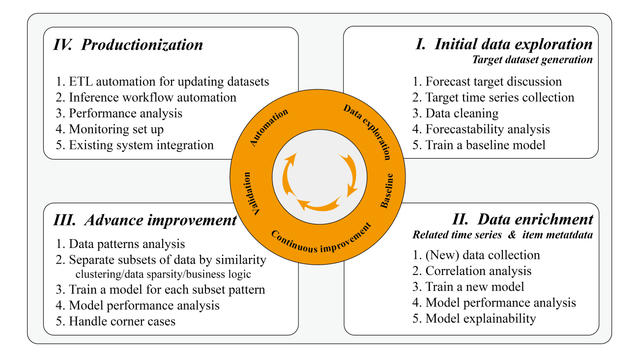
Minghui Yu is a Senior Machine Learning Team Lead for Inference at ByteDance. His focus area is AI Computing Acceleration and Machine Learning System. He is very interested in heterogeneous computing and computer architecture in the post Moore era. In his spare time, he likes basketball and archery.

Jianzhe Xiao is a Senior Software Engineer Team Lead in AML Team at ByteDance. His current work focuses on helping the business team speed up the model deploy process and improve the model’s inference performance. Outside of work, he enjoys playing the piano.

Tian Shi is a Senior Solutions Architect at AWS. His focus area is data analytics, machine learning and serverless. He is passionate about helping customers design and build reliable and scalable solutions on the cloud. In his spare time, he enjoys swimming and reading.

Jia Dong is Customer Solutions Manager at AWS. She enjoys learning about AWS AI/ML services and helping customers meet their business outcomes by building solutions for them. Outside of  work, Jia enjoys travel, Yoga and movies.

Jonathan Lunt is a software engineer at Amazon with a focus on ML framework development. Over his career he has worked through the full breadth of data science roles including model development, infrastructure deployment, and hardware-specific optimization.

Joshua Hannan is a machine learning engineer at Amazon. He works on optimizing deep learning models for large-scale computer vision and natural language processing applications.

Shruti Koparkar is a Senior Product Marketing Manager at AWS. She helps customers explore, evaluate, and adopt EC2 accelerated computing infrastructure for their machine learning needs.

Read More

Companies that sell products or services online need to constantly monitor customer reviews left on their website after purchasing a product. The company’s marketing and customer service departments analyze these reviews to understand customer sentiment. For example, marketing could use this data to create campaigns targeting different customer segments. Customer service departments could use this data to spot customer dissatisfaction and take corrective action.

Traditionally, this data is collected via a batch process and sent to a data warehouse for storage, analysis, and reporting, and is made available to decision-makers after several hours, if not days. If this data can be analyzed immediately, it can provide opportunities for companies to react quickly to customer sentiment.

In this post, we describe an approach for analyzing the overall sentiment of customer feedback in near-real time (a few minutes). We also demonstrate how to understand the different sentiments associated with specific entities in the text (such as company, product, person, or brand) directly from the API.

Use cases for real-time sentiment analysis

Real-time sentiment analysis is very useful for companies interested in getting instant customer feedback on their products and services, such as:

• Restaurants
• Retail or B2C companies selling various products or services
• Companies streaming online movies (OTT platforms), live concerts, or sports events
• Financial institutions

In general, any business that has customer touchpoints and needs to make real-time decisions can benefit from real-time feedback from customers.

Deploying a real-time approach to sentiment can be useful in the following use cases:

• Marketing departments can use the data to target customer segments better, or adjust their campaigns to specific customer segments.
• Customer service departments can reach out to dissatisfied customers immediately and try to resolve the problems, preventing customer churn.
• Positive or negative sentiment on a product can prove as a useful indicator of product demand in various locations. For example, for a fast-moving product, companies can use the real-time data to adjust their stock levels in warehouses, to avoid excess inventory or stockouts in specific regions.

It’s also useful to have a granular understanding of sentiment, as in the following use cases:

• A business can identify parts of the employee/customer experience that are enjoyable and parts that may be improved.
• Contact centers and customer service teams can analyze on-call transcriptions or chat logs to identify agent training effectiveness, and conversation details such as specific reactions from a customer and phrases or words that were used to elicit that response.
• Product owners and UI/UX developers can identify features of their product that users enjoy and parts that require improvement. This can support product roadmap discussions and prioritizations.

Solution overview

We present a solution that can help companies analyze customer sentiment (both full and targeted) in near-real time (usually in a few minutes) from reviews entered on their website. At its core, it relies on Amazon Comprehend to perform both full and targeted sentiment analysis.

The Amazon Comprehend sentiment API identifies the overall sentiment for a text document. As of October 2022, you can use targeted sentiment to identify the sentiment associated with specific entities mentioned in text documents. For example, in a restaurant review that says, “I loved the burger but the service was slow,” the targeted sentiment will identify positive sentiment for “burger” and negative sentiment for “service.”

For our use case, a large restaurant chain in North America wants to analyze reviews made by their customers on their website and via a mobile app. The restaurant wants to analyze their customers’ feedback on various items in the menu, the service provided at their branches, and the overall sentiment on their experience.

For example, a customer could write the following review: “The food at your restaurant located in New York was very good. The pasta was delicious. However, the service was very poor!” For this review, the location of the restaurant is New York. The overall sentiment is mixed—the sentiment for “food” and “pasta” is positive, but the sentiment for the service is negative.

The restaurant wants to analyze the reviews by customer profile, such as age and gender, to identify any trends across customer segments (this data could be captured by their web and mobile apps and sent to the backend system). Their customer service department wants to use this data to notify agents to follow up on the issue by creating a customer ticket in a downstream CRM system. Operations wants to understand which items are fast moving on a given day, so they can reduce the preparation time for those items.

Currently, all the analyses are delivered as reports by email via a batch process that takes 2–3 days. The restaurant’s IT department lacks sophisticated data analytics, streaming, or AI and machine learning (ML) capabilities to build such a solution.

The following architecture diagram illustrates the first steps of the workflow.

First steps of the workflow

The entire solution can be hooked to the back of a customer website or a mobile app.

Amazon API Gateway exposes two endpoints:

• A customer endpoint where customer reviews are entered
• A service endpoint where a service department can look at any particular review and create a service ticket

The workflow includes the following steps:

1. When a customer enters a review (for example, from the website), it’s sent to an API Gateway that is connected to an Amazon Simple Queue Service (Amazon SQS) queue. The queue acts as a buffer to store the reviews as they are entered.
2. The SQS queue triggers an AWS Lambda function. If the message is not delivered to the Lambda function after a few retry attempts, it’s placed in the dead-letter queue for future inspection.
3. The Lambda function invokes the AWS Step Functions state machine and passes the message from the queue.

The following diagram illustrates the Step Functions workflow.

Step Functions Workflow

Step Functions does the following steps in parallel.

1. Step Functions analyzes the full sentiment of the message by invoking the detect_sentiment API from Amazon Comprehend.
2. It invokes the following steps:
   1. It writes the results to an Amazon DynamoDB table.
   2. If the sentiment is negative or mixed, it performs the following actions:
      • It sends a notification to Amazon Simple Notification Service (Amazon SNS), which is subscribed by one or more email addresses (such as the Director of Customer Service, Director of Marketing, and so on).
      • It sends an event to Amazon EventBridge, which is passed on to another downstream systems to act on the review received. In the example, the EventBridge event is written to an Amazon CloudWatch log. In a real scenario, it could invoke a Lambda function to send the event to a downstream system inside or outside AWS (such as an inventory management system or scheduling system).
3. It analyzes the targeted sentiment of the message by invoking the detect_targeted_sentiment API from Amazon Comprehend.
4. It writes the results to a DynamoDB table using the Map function (in parallel, one for each entity identified in the message).

The following diagram illustrates the workflow from Step Functions to downstream systems.

Step Functions to downstream systems

1. The DynamoDB tables use Amazon DynamoDB Streams to perform change data capture (CDC). The data inserted into the tables is streamed via Amazon Kinesis Data Streams to Amazon Kinesis Data Firehose in near-real time (set to 60 seconds).
2. Kinesis Data Firehose deposits the data into an Amazon Simple Storage Service (Amazon S3) bucket.
3. Amazon QuickSight analyzes the data in the S3 bucket. The results are presented in various dashboards that can be viewed by sales, marketing, or customer service teams (internal users). QuickSight can also refresh the dashboard on a schedule (set to 60 minutes for this example).

The AWS CloudFormation templates to create the solution architecture are available on GitHub. Note that the templates don’t include the QuickSight dashboards, but provide instructions on how to create them in the README.md file. We provide some sample dashboards in the following section.

QuickSight dashboards

Dashboards are useful for marketing and customer service departments to visually analyze how their product or service is doing across key business metrics. In this section, we present some sample reports that were developed in QuickSight, using fictitious data for the restaurant. These reports are available to decision-makers in about 60 minutes (as per our refresh cycle). They can help answer questions like the following:

• How are customers perceiving the business as a whole?
• Are there any specific aspects of the service (such as time taken to deliver service, resolution provided on a customer complaint) that customers like or don’t like?
• How do customers like a specific newly introduced product (such as an item on the menu)? Are there any specific products that customers like or don’t like?
• Are there any observable patterns in customer sentiment across age groups, gender, or locations (such as what food items are popular in various locations today)?

Full sentiment

The following figures show examples of full sentiment analysis.

The first graph is of the overall sentiment.

Full sentiment

The next graph shows the sentiment across age groups.

Sentiment across age groups

The following graph shows sentiment across gender.

Sentiment across gender

The final graph shows sentiment across restaurant locations.

Sentiment across locations

Targeted sentiment

The following figures show examples of targeted sentiment analysis.

The first graph shows sentiment by entity (service, restaurant, types of meal, and so on).

Targeted sentiment by entity

The following shows sentiment across age groups by entity.

Sentiment across age groups by entity

The next graph shows sentiment across locations by entity.

Sentiment across locations by entity

The following screenshot is from a CRM ticketing system that could be used for more granular analysis of customer sentiment. For example, in our use case, we set up the customer service department to receive email notifications of negative sentiments. With the information from the email (the review ID of the customer sentiment), a service representative can drill down to more granular details of the sentiment.

CRM ticketing system

Summary

This post described an architecture for real-time sentiment analysis using Amazon Comprehend and other AWS services. Our solution provides the following benefits:

• It’s delivered as a CloudFormation template with an API Gateway that can be deployed behind customer-facing apps or mobile apps
• You can build the solution using Amazon Comprehend, with no special knowledge of AI, ML, or natural language processing
• You can build reports using QuickSight with no special knowledge of SQL
• It can be completely serverless, which provides elastic scaling and consumes resources only when needed

Real-time sentiment analysis can be very useful for companies interested in getting instant customer feedback on their services. It can help the company’s marketing, sales, and customer service departments instantly review customer feedback and take corrective actions.

Use this solution in your company to detect and react to customer sentiments in near-real time.

To learn more about the key services described in this blog, visit the links below

Amazon Comprehend
AWS Step Functions
Amazon DynamoDB Streams
Amazon Kinesis Data Streams
Amazon Kinesis Data Firehose
Amazon EventBridge
Amazon QuickSight

About the Author

Varad G Varadarajan is a Senior Solutions Architect (SA) at Amazon Web Services, supporting customers in the US North East. Varad acts as a Trusted Advisor and Field CTO for Digital Native Businesses, helping them build innovative solutions at scale, using AWS. Varad’s areas of interest are IT Strategy Consulting, Architecture and Product Management. Outside of work, Varad enjoys creative writing, watching movies with family and friends, and traveling.

Read More

Amazon Rekognition offers pre-trained and customizable computer vision capabilities to extract information and insights from images and videos. One such capability is Amazon Rekognition Labels, which detects objects, scenes, actions, and concepts in images. Customers such as Synchronoss, Shutterstock, and Nomad Media use Amazon Rekognition Labels to automatically add metadata to their content library and enable content-based search results. TripleLift uses Amazon Rekognition Labels to determine the best moments to dynamically insert ads that complement the viewing experience for the audience. VidMob uses Amazon Rekognition Labels to extract metadata from ad creatives to understand the unique role of creative decision-making in ad performance, so marketers can produce ads that impact key objectives they care about most. Additionally, thousands of other customers use Amazon Rekognition Labels to support many other use cases, such as classifying trail or hiking photos, detecting people or vehicles in security camera footage, and classifying identity document pictures.

Amazon Rekognition Labels for images detects 600 new labels, including landmarks and activities, and improves accuracy for over 2,000 existing labels. In addition, Amazon Rekognition Labels now supports Image Properties to detect dominant colors of an image, its foreground and background, as well as detected objects with bounding boxes. Image Properties also measures image brightness, sharpness, and contrast. Lastly, Amazon Rekognition Labels now organizes label results using two additional fields, aliases and categories, and supports filtering of those results. In the following sections, we review the new capabilities and their benefits in more detail with some examples.

New labels

Amazon Rekognition Labels has added over 600 new labels, expanding the list of supported labels. The following are some examples of the new labels:

• Popular landmarks – Brooklyn Bridge, Colosseum, Eiffel Tower, Machu Picchu, Taj Mahal, etc.
• Activities – Applause, Cycling, Celebrating, Jumping, Walking Dog, etc.
• Damage detection – Car Dent, Car Scratch, Corrosion, Home Damage, Roof Damage, Termite Damage, etc.
• Text and documents – Bar Chart, Boarding Pass, Flow Chart, Notebook, Invoice, Receipt, etc.
• Sports – Baseball Game, Cricket Bat, Figure Skating, Rugby, Water Polo, etc.
• Many more – Boat Racing, Fun, Cityscape, Village, Wedding Proposal, Banquet, etc.

With these labels, customers in image sharing, stock photography, or broadcast media can automatically add new metadata to their content library to improve their search capabilities.

Let’s look at a label detection example for the Brooklyn Bridge.

The following table shows the labels and confidence scores returned in the API response.

Improved labels

Amazon Rekognition Labels has also improved the accuracy for over 2,000 labels. The following are some examples of the improved labels:

• Activities – Diving, Driving, Reading, Sitting, Standing, etc.
• Apparel and accessories – Backpack, Belt, Blouse, Hoodie, Jacket, Shoe, etc.
• Home and indoors – Swimming Pool, Potted Plant, Pillow, Fireplace, Blanket, etc.
• Technology and computing – Headphones, Mobile Phone, Tablet Computer, Reading, Laptop, etc.
• Vehicles and automotive – Truck, Wheel, Tire, Bumper, Car Seat, Car Mirror, etc.
• Text and documents – Passport, Driving License, Business Card, Document, etc.
• Many more – Dog, Kangaroo, Town Square, Festival, Laughing, etc.

Image Properties for dominant color detection and image quality

Image Properties is a new capability of Amazon Rekognition Labels for images, and can be used with or without the label detection functionality. Note: Image Properties is priced separately from Amazon Rekognition Labels, and is only available with the updated SDKs.

Dominant color detection

Image Properties identifies dominant colors in an image based on pixel percentages. These dominant colors are mapped to the 140 CSS color palette, RGB, hex code, and 12 simplified colors (green, pink, black, red, yellow, cyan, brown, orange, white, purple, blue, grey). By default, the API returns up to 10 dominant colors unless you specify the number of colors to return. The maximum number of dominant colors the API can return is 12.

When used standalone, Image Properties detects the dominant colors of an entire image as well as its foreground and background. When used together with label detection functionalities, Image Properties also identifies the dominant colors of detected objects with bounding boxes.

Customers in image sharing or stock photography can use dominant color detection to enrich their image library metadata to improve content discovery, allowing their end-users to filter by color or search objects with specific colors, such as “blue chair” or “red shoes.” Additionally, customers in advertising can determine ad performance based on the colors of their creative assets.

Image quality

In addition to dominant color detection, Image Properties also measures image qualities through brightness, sharpness, and contrast scores. Each of these scores ranges from 0–100. For example, a very dark image will return low brightness values, whereas a brightly lit image will return high values.

With these scores, customers in image sharing, advertising, or ecommerce can perform quality inspection and filter out images with low brightness and sharpness to reduce false label predictions.

The following image shows an example with the Eiffel Tower.

The following table is an example of Image Properties data returned in the API response.

The following image is an example for a red chair.

The following is an example of Image Properties data returned in the API response.

The following image is an example for a dog with a yellow background.

The following is an example of Image Properties data returned in the API response.

New aliases and categories fields

Amazon Rekognition Labels now returns two new fields, aliases and categories, in the API response. Aliases are other names for the same label and categories group individual labels together based on 40 common themes, such as Food and Beverage and Animals and Pets. With the label detection model update, aliases are no longer returned in the primary list of label names. Instead, aliases are returned in the new aliases field in the API response. Note: Aliases and categories are only returned with the updated SDKs.

Customers in photo sharing, ecommerce, or advertising can use aliases and categories to organize their content metadata taxonomy to further enhance content search and filtering:

• Aliases example – Because Car and Automobile are aliases, you can add metadata to an image with Car and Automobile at the same time
• Categories example – You can use categories to create a category filter or display all images related to a particular category, such as Food and Beverage, without having to explicitly add metadata to each image with Food and Beverage

The following image shows a label detection example with aliases and categories for a diver.

The following table shows the labels, confidence scores, aliases, and categories returned in the API response.

The following image is an example for a cyclist.

The following table contains the labels, confidence scores, aliases, and categories returned in the API response.

Inclusion and exclusion filters

Amazon Rekognition Labels introduces new inclusion and exclusion filtering options in the API input parameters to narrow down the specific list of labels returned in the API response. You can provide an explicit list of labels or categories that you want to include or exclude. Note: These filters are available with the updated SDKs.

Customers can use inclusion and exclusion filters to obtain specific labels or categories they are interested in without having to create additional logic in their application. For example, customers in insurance can use LabelCategoriesInclusionFilter to only include label results in the Damage Detection category.

The following code is an API sample request with inclusion and exclusion filters:

{
    "Image": {
        "S3Object": {
            "Bucket": "bucket",
            "Name": "input.jpg" 
        } 
    },
    "MaxLabels": 10, 
    "MinConfidence": 75,
    "Features": [ "GENERAL_LABELS", "IMAGE_PROPERTIES" ],
    "Settings": {
        "GeneralLabels": {
            "LabelsInclusionFilter": [<Label(s)>],
            "LabelsExclusionFilter": [<Label(s)>],
            "LabelCategoriesInclusionFilter": [<Category Name(s)>],
            "LabelCategoriesExclusionFilter": [<Category Name(s)>] 
        },
        "ImageProperties": {
            "MaxDominantColors":10
        }
    }
 }

The following are examples of how inclusion and exclusion filters work:

• If you only want to detect Person and Car, and don’t care about other labels, you can specify [“Person”,”Car”] in LabelsInclusionFilter.
• If you want to detect all labels except for Clothing, you can specify [“Clothing”] in LabelsExclusionFilter.
• If you want to detect only labels within the Animal and Pets categories except for Dog and Cat, you can specify ["Animal and Pets"] in the LabelCategoriesInclusionFilter, with ["Dog", "Cat"] in LabelsExclusionFilter.
• If a label is specified in LabelsInclusionFilter or LabelsExclusionFilter, their aliases will be included or excluded accordingly because aliases is a sub-taxonomy of labels. For example, because Automobile is an alias of Car, if you specify Car in LabelsInclusionFilter, the API will return the Car label with Automobile in the aliases field.

Conclusion

Amazon Rekognition Labels detects 600 new labels and improves accuracy for over 2,000 existing labels. Along with these updates, Amazon Rekognition Labels now supports Image Properties, aliases and categories, as well as inclusion and inclusion filters.

To try the new label detection model with its new features, log in to your AWS account and check out the Amazon Rekognition console for label detection and image properties. To learn more, visit Detecting labels.

About the authors

Maria Handoko is a Senior Product Manager at AWS. She focuses on helping customers solve their business challenges through machine learning and computer vision. In her spare time, she enjoys hiking, listening to podcasts, and exploring different cuisines.

Shipra Kanoria is a Principal Product Manager at AWS. She is passionate about helping customers solve their most complex problems with the power of machine learning and artificial intelligence. Before joining AWS, Shipra spent over 4 years at Amazon Alexa, where she launched many productivity-related features on the Alexa voice assistant.

Read More