What’s new in TensorFlow 2.11?

What’s new in TensorFlow 2.11?

Posted by the Tensor Flow Team

TensorFlow 2.11 has been released! Highlights of this release include enhancements to DTensor, the completion of the Keras Optimizer migration, the introduction of an experimental StructuredTensor, a new warmstart embedding utility for Keras, a new group normalization Keras layer, native TF Serving support for TensorFlow Decision Forest models, and more. Let’s take a look at these new features.

TensorFlow Core

DTensor

DTensor is a TensorFlow API for distributed processing that allows models to seamlessly move from data parallelism to single program multiple data (SPMD) based model parallelism, including spatial partitioning. It gives you tools to easily train models where the model weights or inputs are so large they don’t fit on a single device. We’ve made several updates in TensorFlow v2.11.

DTensor supports tf.train.Checkpoint
You can now checkpoint a DTensor model using tf.train.Checkpoint. Saving and restoring sharded DVariables will perform an efficient sharded save and restore. All DVariables must have the same host mesh, and DVariables and regular variables cannot be saved together. The old DCheckpoint based checkpointing API will be removed in the next release. You can learn more about checkpointing in this tutorial.

A new unified accelerator initialization API
We’ve introduced a new unified accelerator initialization API tf.experimental.dtensor.initialize_accelerator_system that shall be called for all three supported accelerator types (CPU, GPU and TPU), and all supported deployment modes (multi-client and local). The old initialization API, which had specialized functions for CPU/GPU multi-client and TPU, will be removed in the next release.
All-reduce optimizations enabled by default
DTensor enables by default an All-reduce optimization pass for GPU and CPU to combine all the independent all-reduces into one. The optimization is expected to reduce overhead of small all-reduce operations, and our experiments showed significant improvements to training step time on BERT. The optimization can be disabled by setting the environment variable ‘DTENSOR_ENABLE_COMBINE_ALL_REDUCES_OPTIMIZATION’ to 0.

A new wrapper for a distributed tf.data.Dataset
We’ve introduced a wrapper for a distributed tf.data.Dataset, tf.experimental.dtensor.DTensorDataset. The DTensorDataset API can be used to efficiently handle loading the input data directly as DTensors by correctly packing it to the corresponding devices. It can be used for both data and model parallel training setups. See the API documentation linked above for more examples.

Keras

The new Keras Optimizers API is ready

In TensorFlow 2.9, we released an experimental version of the new Keras Optimizer APItf.keras.optimizers.experimental, to provide a more unified and expanded catalog of built-in optimizers which can be more easily customized and extended. In TensorFlow 2.11, we’re happy to share that the Optimizer migration is complete, and the new optimizers are on by default.

The old Keras Optimizers are available under tf.keras.optimizers.legacy. These will never be deleted, but they will not see any new feature additions. New optimizers will only be implemented based on tf.keras.optimizers.Optimizer, the new base class.

Most users won’t be affected by this change, but if you find your workflow failing, please check out the release notes for possible issues, and the API doc to see if any API used in your workflow has changed.

The new GroupNormalization layer

TensorFlow 2.11 adds a new group normalization layer, keras.layers.GroupNormalization. Group Normalization divides the channels into groups and computes within each group the mean and variance for normalization. Empirically, its accuracy can be more stable than batch norm in a wide range of small batch sizes, if learning rate is adjusted linearly with batch sizes. See the API doc for more details, and try it out!

A diagram showing the differences between normalization techniques.

Warmstart embedding utility

TensorFlow 2.11 includes a new utility function: keras.utils.warmstart_embedding_matrix. It lets you initialize embedding vectors for a new vocabulary from another set of embedding vectors, usually trained on a previous run.

new_embedding = layers.Embedding(vocab_size, embedding_depth)
new_embedding.build(input_shape=[None])
new_embedding.embeddings.assign(
    tf.keras.utils.warmstart_embedding_matrix(
        base_vocabulary=base_vectorization.get_vocabulary(),
        new_vocabulary=new_vectorization.get_vocabulary(),
        base_embeddings=base_embedding.embeddings,
        new_embeddings_initializer=“uniform”)

See the Warmstart embedding tutorial for a full walkthrough.

TensorFlow Decision Forests

With the release of TensorFlow 2.11, TensorFlow Serving adds native support for TensorFlow Decision Forests models. This greatly simplifies serving TF-DF models in Google Cloud and other production systems. Check out the new TensorFlow Decision Forests and TensorFlow Serving tutorial, and the new Making predictions tutorial, to learn more.

And did you know that TF-DF comes preinstalled in Kaggle notebooks? Simply import TF-DF with import tensorflow_decision_forests as tfdf and start modeling.

TensorFlow Lite

TensorFlow Lite now supports new operations including tf.unsorted_segment_min, tf.atan2 and tf.sign. We’ve also updated tfl.mul to support complex32 inputs.

Structured Tensor

The tf.experimental.StructuredTensor class has been added. This class provides a flexible and TensorFlow-native way to encode structured data such as protocol buffers or pandas dataframes. StructuredTensor allows you to write readable code that can be used with tf.function, Keras, and tf.data. Here’s a quick example.

documents = tf.constant([
    “Hello world”,
    “StructuredTensor is cool”])

@tf.function
def parse_document(documents):
tokens = tf.strings.split(documents)
token_lengths = tf.strings.length(tokens)

ext_tokens = tf.experimental.StructuredTensor.from_fields_and_rank(
    {“tokens”:tokens,
      “length”:token_lengths}, rank=documents.shape.rank + 1)

return tf.experimental.StructuredTensor.from_fields_and_rank({
    “document”:documents,
    “tokens”:ext_tokens}, rank=documents.shape.rank)

st = parse_document(documents)

A StructuredTensor can be accessed either by index, or by field name(s).

>>> st[0].to_pyval()
{‘document’: b’Hello world’,
‘tokens’: [{‘length’: 5, ‘token’: b’Hello’},
  {‘length’: 5, ‘token’: b’world’}]}

Under the hood, the fields are encoded as Tensors and RaggedTensors.

>>> st.field_value((“tokens”, “length”))

<tf.RaggedTensor [[5, 5], [16, 2, 4]]>

You can learn more in the API doc linked above.

Coming soon

Deprecating Estimator and Feature Column

Effective with the release of TensorFlow 2.12, TensorFlow 1’s Estimator and Feature Column APIs will be considered fully deprecated, in favor of their robust and complete equivalents in Keras. As modules running v1.Session-style code, Estimators and Feature Columns are difficult to write correctly and are especially prone to behave unexpectedly, especially when combined with code from TensorFlow 2.

As the primary gateways into most of the model development done in TensorFlow 1, we’ve taken care to ensure their replacements have feature parity and are actively supported. Going forward, model building with Estimator APIs should be migrated to Keras APIs, with feature preprocessing via Feature Columns specifically migrated to Keras’s preprocessing layers – either directly or through the TF 2.12 one-stop utility tf.keras.utils.FeatureSpace built on top of them.

Deprecation will be reflected throughout the TensorFlow documentation as well as via warnings raised at runtime, both detailing how to avoid the deprecated behavior and adopt its replacement.

Deprecating Python 3.7 Support after TF 2.11

TensorFlow 2.11 will be the last TF version to support Python 3.7. Since TensorFlow depends on NumPy, we are aiming to follow numpy’s Python version support policy which will benefit our internal and external users and keep our software secure. Additionally, a few vulnerabilities reported recently required that we bump our numpy version, which turned out not compatible with Python 3.7, further supporting the decision to drop support for Python 3.7.

Next steps

Check out the release notes for more information. To stay up to date, you can read the TensorFlow blog, follow twitter.com/tensorflow, or subscribe to youtube.com/tensorflow. If you’ve built something you’d like to share, please submit it for our Community Spotlight at goo.gle/TFCS. For feedback, please file an issue on GitHub or post to the TensorFlow Forum. Thank you!

Read More

Startup Uses Speech AI to Coach Contact-Center Agents Into Boosting Customer Satisfaction

Startup Uses Speech AI to Coach Contact-Center Agents Into Boosting Customer Satisfaction

Minerva CQ, a startup based in the San Francisco Bay Area, is making customer service calls quicker and more efficient for both agents and customers, with a focus on those in the energy sector.

The NVIDIA Inception member’s name is a mashup of the Roman goddess of wisdom and knowledge — and collaborative intelligence (CQ), or the combination of human and artificial intelligence.

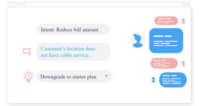
The Minerva CQ platform coaches contact-center agents to drive customer conversations — whether in voice or web-based chat — toward the most effective resolutions by offering real-time dialogue suggestions, sentiment analysis and optimal journey flows based on the customer’s intent. It also surfaces relevant context, articles, forms and more.

Powered by the NVIDIA Riva software development kit, Minerva CQ has best-in-class automatic speech recognition (ASR) capabilities in English, Spanish and Italian.

“Many contact-center solutions focus on automation through a chatbot, but our solution lets the AI augment humans to do a better job, because when humans and machines work together, they can accomplish more than what the human or machine alone could,” said Cosimo Spera, founder and CEO of Minerva CQ.

The platform first transcribes a conversation into text in real time. That text is then fed into Minerva CQ’s AI models that analyze customer sentiment, intent, propensity and more.

Minerva CQ then offers agents the best path to help their customers, along with other optional resolution paths.

The speech AI platform can understand voice- and text-based conversations within both the context of a specific exchange and the customer’s broader relationship with the business, according to Jack Garrett, vision architect at Minerva CQ.

Watch a demo of Minerva CQ at work:

Speech AI Powered by NVIDIA Riva

Minerva CQ last month announced that it built what it says is the first and most accurate Italian ASR model for enterprises, adding to the platform’s existing English and Spanish capabilities. The Italian ASR model has a word error rate of under 7% and is expected to be deployed early next year at a global energy company and telecoms provider.

“When we were looking for the best combination of accuracy, speed and cost to help us build the ASR model, NVIDIA Riva was at the top of our list,” Spera said.

Riva enables Minerva CQ to offer real-time responses. This means the AI platform can stream, process and transcribe conversations — all in less than 300 milliseconds, or in a blink of an eye.

“Riva is also fully customizable to solve our customers’ unique problems and comes with industry-leading out-of-the-box accuracy,” said Daniel Hong, chief marketing officer at Minerva CQ. “We were able to quickly and efficiently fine-tune the pretrained language models with help from experts on the NVIDIA Riva team.”

Access to technical experts is one benefit of being part of NVIDIA Inception, a free, global program that nurtures cutting-edge startups. Spera listed AWS credits, support on experimental projects, and collaboration on go-to-market strategy among the ways Inception has bolstered Minerva CQ.

In addition to Riva, Minerva CQ uses the NVIDIA NeMo framework to build and train its conversational AI models, as well as the NVIDIA Triton Inference Server to deliver fast, scalable AI model deployment.

Complementing its focus on the customer, Minerva CQ is also dedicated to agent wellness and building capabilities to track agent satisfaction and experience. The platform enables employees to be experts at their jobs from day one — which greatly reduces stress on agents, instills confidence, and lowers attrition rates and operational costs.

Plus, Minerva CQ automatically provides summary reports of conversations, giving agents and supervisors helpful feedback, and analytics teams powerful business insights.

“All in all, Minerva CQ empowers agents with knowledge and allows them to be confident in the information they share with customers,” Hong said. “Easy customer inquiries can be tackled by automated self-service or AI chatbots, so when the agents are hit with complex questions, Minerva can help.”

Focus on Retail Energy, Electrification

Minerva CQ’s initial deployments are focused on retail energy and electrification.

For retail energy providers, the platform offers agents simple, consistent explanations of energy sources, tariff plans, billing changes and optimal spending choices.

It also assists agents to resolve complex problems for electric vehicle customers, and helps EV technicians troubleshoot infrastructure and logistics issues.

“Retail energy and electrification are inherently intertwined in the movement toward decarbonization, but they can still be relatively siloed in the market space,” Garrett said. “Minerva helps bring them together.”

Minerva CQ is deployed by a leading electric mobility company as well as one of the largest utilities in the world, according to Spera.

These clients’ contact centers across the U.S. and Mexico have seen a 40% decrease in average handle time for a customer service call thanks to Minerva CQ, Spera said. Deployment is planned to expand further into the Spanish-speaking market — as well as in countries where Italian is spoken.

“We all want to save the planet, but it’s important that change come from the bottom up by empowering end users to make steps toward decarbonization,” Spera said. “Our focus is on providing customers with information so they can best transition to clean-energy-source subscriptions.”

He added, “In the coming years, we’d like to see the brand Minerva CQ become synonymous with electrification and decarbonization.”

Learn more about NVIDIA’s work with utilities and apply to join NVIDIA Inception.

The post Startup Uses Speech AI to Coach Contact-Center Agents Into Boosting Customer Satisfaction appeared first on NVIDIA Blog.

Read More

Scaling Multimodal Foundation Models in TorchMultimodal with Pytorch Distributed

Scaling Multimodal Foundation Models in TorchMultimodal with Pytorch Distributed

Introduction

In recent years, scaling model sizes has become a promising area of research. In the field of NLP, language models have gone from hundreds of millions of parameters (BERT) to hundreds of billions of parameters (GPT-3) demonstrating significant improvements on downstream tasks. The scaling laws for large scale language models have also been studied extensively in the industry. A similar trend can be observed in the vision field, with the community moving to transformer based models (like Vision Transformer, Masked Auto Encoders) as well. It is clear that individual modalities – text, image, video – have benefited massively from recent advancements in scale, and frameworks have quickly adapted to accommodate larger models.

At the same time, multimodality is becoming increasingly important in research with tasks like image-text retrieval, visual question-answering, visual dialog and text to image generation gaining traction in real world applications. Training large scale multimodal models is the natural next step and we already see several efforts in this area like CLIP from OpenAI, Parti from Google and CM3 from Meta.

In this blog, we present a case study demonstrating the scaling of FLAVA to 10B params using techniques from PyTorch Distributed. FLAVA is a vision and language foundation model, available in TorchMultimodal, which has shown competitive performance on both unimodal and multimodal benchmarks. We also give the relevant code pointers in this blog. The instructions for running an example script to scale FLAVA can be found here.

Scaling FLAVA Overview

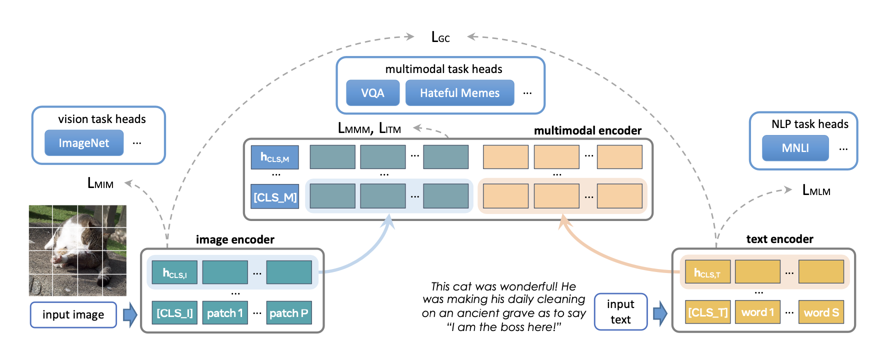
FLAVA is a foundation multimodal model which consists of transformer based image and text encoders followed by a transformer-based multimodal fusion module. It is pretrained on both unimodal and multimodal data with a diverse set of losses. This includes masked language, image and multimodal modeling losses that require the model to reconstruct the original input from its context (self-supervised learning). It also uses image text matching loss over positive and negative examples of aligned image-text pairs as well as CLIP style contrastive loss. In addition to multimodal tasks (like image-text retrieval), FLAVA demonstrated competitive performance on unimodal benchmarks as well (GLUE tasks for NLP and image classification for vision).

The original FLAVA model has ~350M parameters and uses ViT-B16 configurations (from the Vision Transformer paper) for image and text encoders. The multimodal fusion transformer follows the unimodal encoders but with half the number of layers. We explore increasing the size of each encoder to larger ViT variants.

Another aspect of scaling is adding the ability to increase the batch size. FLAVA makes use of contrastive loss over in-batch negatives, which typically benefits from large batch size (as studied here). The largest training efficiency or throughput is also generally achieved when operating near maximum possible batch sizes as determined by the amount of GPU memory available (also see the experiments section).

The following table displays the different model configurations we experimented with. We also determine the maximum batch size that was able to fit in memory for each configuration in the experiments section.

Approx Model params Hidden size MLP size Heads Unimodal layers Multimodal layers Model size (fp32)
350M (original) 768 3072 12 12 6 1.33GB
900M 1024 4096 16 24 12 3.48GB
1.8B 1280 5120 16 32 16 6.66GB
2.7B 1408 6144 16 40 20 10.3GB
4.8B 1664 8192 16 48 24 18.1GB
10B 2048 10240 16 64 40 38GB

Optimization overview

PyTorch offers several native techniques to efficiently scale models. In the following sections, we go over some of these techniques and show how they can be applied to scale up a FLAVA model to 10 billion parameters.

Distributed Data Parallel

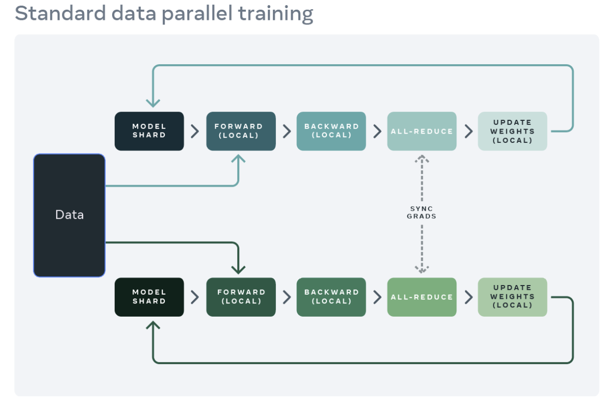
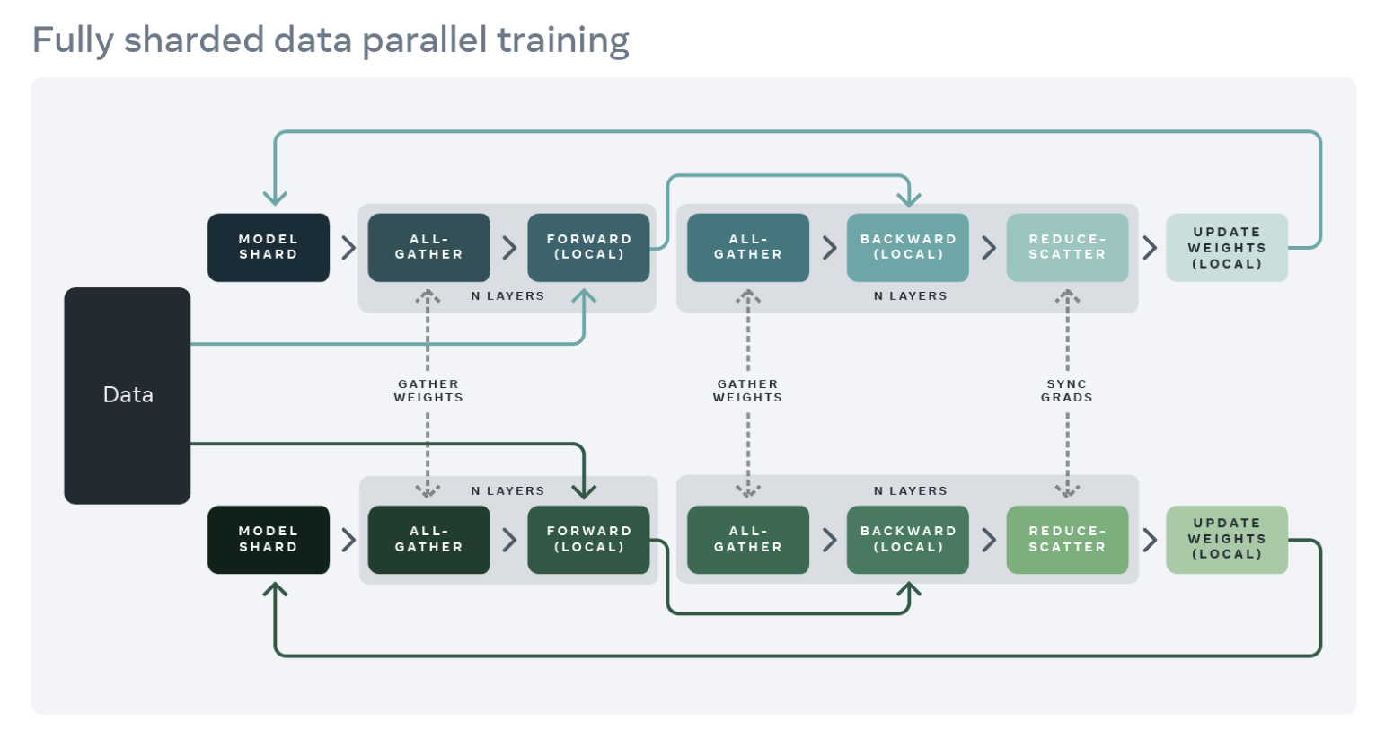
A common starting point for distributed training is data parallelism. Data parallelism replicates the model across each worker (GPU), and partitions the dataset across the workers. Different workers process different data partitions in parallel and synchronize their gradients (via all reduce) before model weights are updated. The figure below showcases the flow (forward, backward, and weight update steps) for processing a single example for data parallelism:

Source: https://engineering.fb.com/2021/07/15/open-source/fsdp/

PyTorch provides a native API, DistributedDataParallel (DDP) to enable data parallelism which can be used as a module wrapper as showcased below. Please see PyTorch Distributed documentation for more details.

from torchmultimodal.models.flava.model import flava_model_for_pretraining
import torch
import torch.distributed as dist

model = flava_model_for_pretraining().cuda()
# Initialize PyTorch Distributed process groups
# Please see https://pytorch.org/tutorials/intermediate/dist_tuto.html for details
dist.init_process_group(backend=”nccl”)
# Wrap model in DDP
model = torch.nn.parallel.DistributedDataParallel(model, device_ids=[torch.cuda.current_device()])

Fully Sharded Data Parallel

GPU memory usage of a training application can roughly be broken down into model inputs, intermediate activations (needed for gradient computation), model parameters, gradients, and optimizer states. Scaling a model will typically increase each of these elements. Scaling a model with DDP can eventually result in out-of-memory issues when a single GPU’s memory becomes insufficient since it replicates the parameters, gradients, and optimizer states on all workers.

To reduce this replication and save GPU memory, we can shard the model parameters, gradients, and optimizer states across all workers with each worker only managing a single shard. This technique was popularized by the ZeRO-3 approach developed by Microsoft. A PyTorch-native implementation of this approach is available as FullyShardedDataParallel (FSDP) API, released as a beta feature in PyTorch 1.12. During a module’s forward and backward passes, FSDP unshards the model parameters as needed for computation (using all-gather) and reshards them after computation. It synchronizes gradients using the reduce-scatter collective to ensure sharded gradients are globally averaged. The forward and backward pass flow of a model wrapped in FSDP are detailed below:

Source: https://engineering.fb.com/2021/07/15/open-source/fsdp/

To use FSDP, the submodules of a model need to be wrapped with the API to control when specific submodules are sharded or unsharded. FSDP provides an auto-wrapping API (see the auto_wrap_policy argument) that can be used out of the box as well as several wrapping policies and the ability to write your own policy.

The following example demonstrates wrapping the FLAVA model with FSDP. We specify the auto-wrapping policy as transformer_auto_wrap_policy. This will wrap individual transformer layers (TransformerEncoderLayer), the image transformer (ImageTransformer), text encoder (BERTTextEncoder) and multimodal encoder (FLAVATransformerWithoutEmbeddings) as individual FSDP units. This uses a recursive wrapping approach for efficient memory management. For example, after an individual transformer layer’s forward or backward pass is finished, its parameters are discarded, freeing up memory thereby reducing peak memory usage.

FSDP also provides a number of configurable options to tune the performance of applications. For example, in our use case, we illustrate the use of the new limit_all_gathers flag, which prevents all-gathering model parameters too early thereby alleviating memory pressure on the application. We encourage users to experiment with this flag which can potentially improve the performance of applications with high active memory usage.

import torch
from torch.distributed.fsdp import FullyShardedDataParallel as FSDP
from torch.distributed.fsdp.wrap import transformer_auto_wrap_policy
from torchmultimodal.models.flava.model import flava_model_for_pretraining
from torchmultimodal.models.flava.text_encoder import BertTextEncoder
from torchmultimodal.models.flava.image_encoder import ImageTransformer
from torchmultimodal.models.flava.transformer import FLAVATransformerWithoutEmbeddings
from torchmultimodal.modules.layers.transformer import TransformerEncoderLayer

model = flava_model_for_pretraining().cuda()
dist.init_process_group(backend=”nccl”)

model = FSDP(
               model,
               device_id=torch.cuda.current_device(),
               auto_wrap_policy=partial(
                   transformer_auto_wrap_policy,
                   transformer_layer_cls={
                       TransformerEncoderLayer,
                       ImageTransformer,
                       BERTTextEncoder,
                       FLAVATransformerWithoutEmbeddings
                   },
               ),
               limit_all_gathers=True,
           )

Activation Checkpointing

As discussed above, intermediate activations, model parameters, gradients, and optimizer states contribute to the overall GPU memory usage. FSDP can reduce memory consumption due to the latter three but does not reduce memory consumed by activations. Memory used by activations increases with increase in batch size or number of hidden layers. Activation checkpointing is a technique to decrease this memory usage by recomputing the activations during the backward pass instead of holding them in memory for a specific checkpointed module. For example, we observed ~4x reduction in the peak active memory after forward pass by applying activation checkpointing to the 2.7B parameter model.

PyTorch offers a wrapper based activation checkpointing API. In particular, checkpoint_wrapper allows users to wrap an individual module with checkpointing, and apply_activation_checkpointing allows users to specify a policy with which to wrap modules within an overall module with checkpointing. Both these APIs can be applied to most models as they do not require any modifications to the model definition code. However, if more granular control over checkpointed segments, such as checkpointing specific functions within a module, is required, the functional torch.utils.checkpoint API can be leveraged, although this requires modification to the model code. The application of the activation checkpointing wrapper to individual FLAVA transformer layers (denoted by TransformerEncoderLayer) is shown below. For a thorough description of activation checkpointing, please see the description in the PyTorch documentation.

from torchmultimodal.models.flava.model import flava_model_for_pretraining
from torch.distributed.algorithms._checkpoint.checkpoint_wrapper import apply_activation_checkpointing, checkpoint_wrapper, CheckpointImpl
from torchmultimodal.modules.layers.transformer import TransformerEncoderLayer

model = flava_model_for_pretraining()
checkpoint_tformer_layers_policy = lambda submodule: isinstance(submodule, TransformerEncoderLayer)

apply_activation_checkpointing(
               model,
               checkpoint_wrapper_fn=checkpoint_wrapper,
               check_fn=checkpoint_tformer_layers_policy,
           )

Used together, wrapping FLAVA transformer layers with activation checkpointing and wrapping the overall model with FSDP as demonstrated above, we are able to scale FLAVA to 10B parameters.

Experiments

We conduct an empirical study about the impact of the different optimizations from the previous section on system performance. For all our experiments, we use a single node with 8 A100 40GB GPUs and run the pretraining for 1000 iterations. All runs also used PyTorch’s automatic mixed precision with the bfloat16 data type. TensorFloat32 format is also enabled to improve matmul performance on the A100. We define throughput as the average number of items (text or image) processed per second (we ignore the first 100 iterations while measuring throughput to account for warmup). We leave training to convergence and its impact on downstream task metrics as an area for future study.

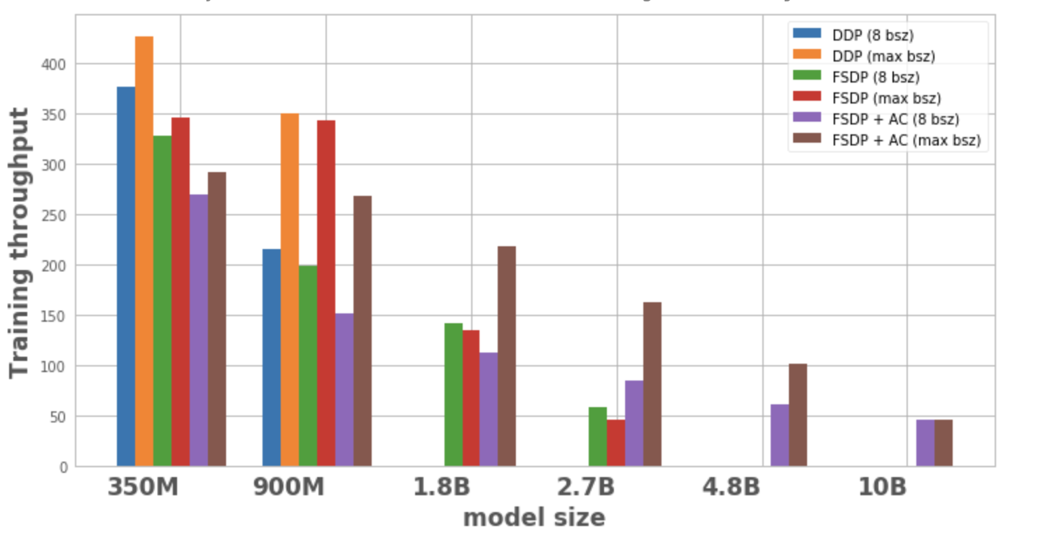
Figure 1 plots the throughput for each model configuration and optimization, both with a local batch size of 8 and then with the maximum batch size possible on 1 node. Absence of a data point for a model variant for an optimization indicates that the model could not be trained on a single node.

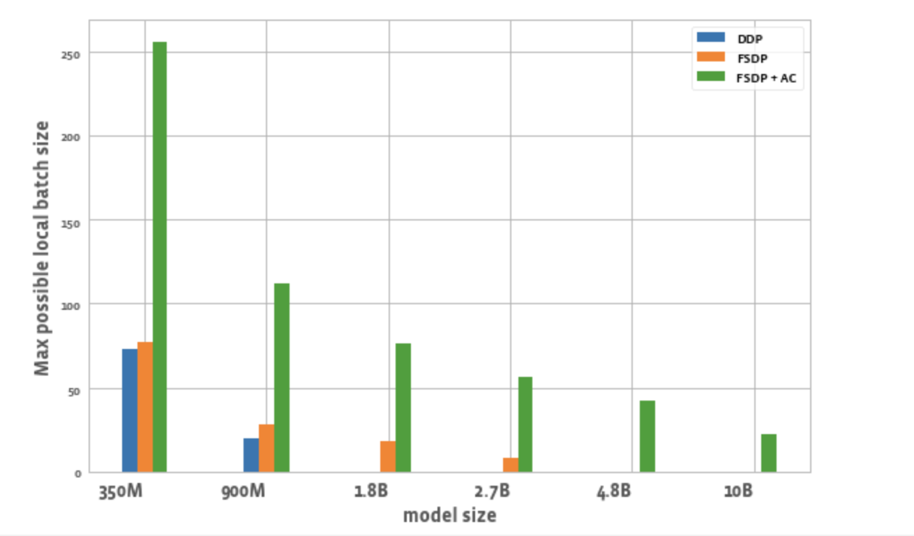
Figure 2 plots the maximum possible batch size per worker for each optimization. We observe a few things:

  1. Scaling model size: DDP is only able to fit the 350M and 900M model on a node. With FSDP, due to memory savings, we are able to train ~3x bigger models compared to DDP (i.e. the 1.8B and 2.7B variants). Combining activation checkpointing (AC) with FSDP enables training even bigger models, on the order of ~10x compared to DDP (i.e. 4.8B and 10B variants)
  2. Throughput:
    • For smaller model sizes, at a constant batch size of 8, the throughput for DDP is slightly higher than or equal to FSDP, explainable by the additional communication required by FSDP. It is lowest for FSDP and AC combined together. This is because AC re-runs checkpointed forward passes during the backwards pass, trading off additional computation for memory savings. However, in the case of the 2.7B model, FSDP + AC actually has higher throughput compared to FSDP alone. This is because the 2.7B model with FSDP is operating close to the memory limit even at batch size 8 triggering CUDA malloc retries which tend to slow down training. AC helps with reducing the memory pressure and leads to no retries.
    • For DDP and FSDP + AC, the throughput increases with an increase in batch size for each model. For FSDP alone, this is true for smaller variants. However, with the 1.8B and 2.7B parameter models, we observe throughput degradation when increasing batch size. A potential reason for this, as noted above also, is that at the memory limit, PyTorch’s CUDA memory management may have to retry cudaMalloc calls and/or run expensive defragmentation steps to find free memory blocks to handle the workload’s memory requirements which can result in training slowdown.
    • For larger models that can only be trained with FSDP (1.8B, 2.7B, 4.8B) the setting with highest throughput achieved is with FSDP + AC scaling to the maximum batch size. For 10B, we observe nearly equal throughput for smaller and maximum batch size. This might be counterintuitive as AC results in increased computation and maxing out batch size potentially leads to expensive defragmentation operations due to operating at CUDA memory limit. However, for these large models, the increase in batch size is large enough to mask this overhead.

Figure 1: Training throughput for different configurations

  1. Batch size: FSDP alone enables slightly higher batch sizes compared to DDP. Using FSDP + AC enables ~3x batch size compared to DDP for the 350M param model and ~5.5x for 900M param model. Even for 10B, a max batch size of ~20 which is fairly decent. This essentially enables larger global batch size using fewer GPUs which is especially useful for contrastive learning tasks.

Figure 2: Max local batchsize possible for different configurations

Conclusion

As the world moves towards multimodal foundation models, scaling model parameters and efficient training is becoming an area of focus. The PyTorch ecosystem aims to accelerate innovation in this field by providing different tools to the research community, both for training and scaling multimodal models. With FLAVA, we laid out an example of scaling a model for multimodal understanding. In the future, we plan to add support for other kinds of models like the ones for multimodal generation and demonstrate their scaling factors. We also hope to automate many of these scaling and memory saving techniques (such as sharding and activation checkpointing) to reduce the amount of user experimentation needed to achieve the desired scale and maximum training throughput.

References

Read More

Homomorphic Self-Supervised Learning

This paper was accepted at the workshop “Self-Supervised Learning – Theory and Practice” at NeurIPS 2022.
Many state of the art self-supervised learning approaches fundamentally rely on transformations applied to the input in order to selectively extract task-relevant information. Recently, the field of equivariant deep learning has developed to introduce structure into the feature space of deep neural networks, specifically with respect to such input transformations. In this work, we observe both theoretically and empirically, that through the lens of equivariant representations, many…Apple Machine Learning Research

Easy and accurate forecasting with AutoGluon-TimeSeries

Easy and accurate forecasting with AutoGluon-TimeSeries

AutoGluon-TimeSeries is the latest addition to AutoGluon, which helps you easily build powerful time series forecasting models with as little as three lines of code.

Time series forecasting is a common task in a wide array of industries as well as scientific domains. Having access to reliable forecasts for supply, demand, or capacity is crucial to planning for businesses. However, time series forecasting is a difficult problem, especially when thousands of potentially related time series are available, such as sales in a large catalog in ecommerce, or capacity at hundreds of operational sites.

Simple statistical or judgement-based forecasting methods are often already strong baselines that are difficult to improve on with novel machine learning (ML) methods. Moreover, applications of recent advances in ML to forecasting are varied, with few methods such as DeepAR [1] or Temporal Fusion Transformers [2] emerging as popular choices. However, these methods are difficult to train, tune, and deploy in production, requiring expert knowledge of ML and time series analysis.

AutoML is a fast-growing topic within ML, focusing on automating common tasks in ML pipelines, including feature preprocessing, model selection, model tuning, ensembling, and deployment. AutoGluon-TimeSeries is the latest addition to AutoGluon, one of the leading open-source AutoML solutions, and builds on AutoGluon’s powerful framework for AutoML in forecasting tasks. AutoGluon-TimeSeries was designed to build powerful forecasting systems with as little as three lines of code, alleviating the challenges of feature preprocessing, model selection, model tuning, and ease of deployment.

With a simple call to AutoGluon-TimeSeries’s TimeSeriesPredictor, AutoGluon follows an intuitive order of priority in fitting models: starting from simple naive baselines and moving to powerful global neural network and boosted tree-based methods, all within the time budget specified by the user. When related time series (time-varying covariates or exogenous variables) or item metadata (static features) are available, AutoGluon-TimeSeries factors them into the forecast. The library also taps into Bayesian optimization for hyperparameter tuning, arriving to the best model configuration by tuning complex models. Finally, AutoGluon-TimeSeries combines the best of statistical and ML-based methods into a model ensemble optimized for the problem at hand.

In this post, we showcase AutoGluon-TimeSeries’s ease of use in quickly building a powerful forecaster.

Get started with AutoGluon-TimeSeries

To start, you need to install AutoGluon, which is easily done with pip on a UNIX shell:

pip install "autogluon>=0.6"

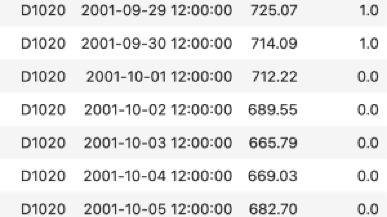
AutoGluon-TimeSeries introduces the TimeSeriesDataFrame class for working with datasets that include multiple related time series (sometimes called a panel dataset). These data frames can be created from so-called long format data frames, which have time series IDs and timestamps arranged into rows. The following is one such data example, taken from the M4 competition [3]. Here, the item_id column specifies the unique identifier of a single time series, such as the product ID for daily sales data of multiple products. The target column is the value of interest that AutoGluon-TimeSeries will learn to forecast. weekend is an extra time-varying covariate we produced to mark if the observation was on the weekend or not.

We can easily produce a new TimeSeriesDataFrame from this dataset using the from_data_frame constructor. See the following Python code:

df = TimeSeriesDataFrame.from_data_frame(raw_data_frame)

Some time series data has non-time-varying features (static features or item metadata) that can be used in training a forecasting model. For example, the M4 dataset features a category variable for each time series. These can be added to the TimeSeriesDataFrame by setting the static_features variable with a new data frame.

Use the following code:

df.static_features = raw_static_features

Train a TimeSeriesPredictor

Finally, we can call the TimeSeriesPredictor to fit a wide array of forecasting models to build an accurate forecasting system. See the following code:

predictor = TimeSeriesPredictor(
    prediction_length=7,
    eval_metric="MASE",
    known_covariates_names=["weekend"],
)

Here, we specify that the TimeSeriesPredictor should produce models to forecast the next seven time periods and judge the best models by using mean absolute scaled error (MASE). Moreover, we indicate that the time-varying covariate weekend is available in the dataset. We can now fit the predictor object on the TimeSeriesDataFrame produced earlier:

predictor.fit(df, presets="medium_quality", time_limit=1800)

Apart from providing the training data, we ask the predictor to use “medium_quality” presets. AutoGluon-TimeSeries comes with multiple presets to select subsets of models to consider and how much time to spend tuning them, managing the trade-off between training speed vs. accuracy. Apart from presets, more experienced users can use a hyperparameters argument to precisely specify component models and which hyperparameters to set on them. We also specify a time limit of 1,800 seconds, after which the predictor stops training.

Under the hood, AutoGluon-TimeSeries trains as many models as it can within the specified time frame, starting from naive but powerful baselines and working towards more complex forecasters based on boosted trees and neural network models. By calling predictor.leaderboard(), we can see a list of all models it has trained and the accuracy scores and training times for each. Note that every AutoGluon-TimeSeries model reports its errors in a “higher is better” format, which means most forecasting error measures are multiplied by -1 when reported. See the following example:

              model  score_val  pred_time_val  fit_time_marginal  fit_order
0  WeightedEnsemble  -0.612510      15.406334          48.428711          8
1  AutoGluonTabular  -0.654924       1.068694         104.208688          6
2            DeepAR  -0.673366       6.731659        1065.956648          7
3     SeasonalNaive  -1.035286       0.410615           0.000742          2
4               ETS  -1.073640       5.832542           0.000584          3
5             Theta  -1.107362       1.773439           0.000614          4
6             ARIMA  -3.006273       2.483140           0.000625          5
7             Naive  -3.427339      29.532215           0.000577          1

Forecast with a TimeSeriesPredictor

Finally, we can use the predictor to predict all time series in a TimeSeriesDataFrame, 7 days into the future. Note that because we used time-varying covariates that are assumed to be known in the future, these should also be specified at prediction time. See the following code:

predictions = predictor.predict(
	df,
	known_covariates=future_known_covariates
)

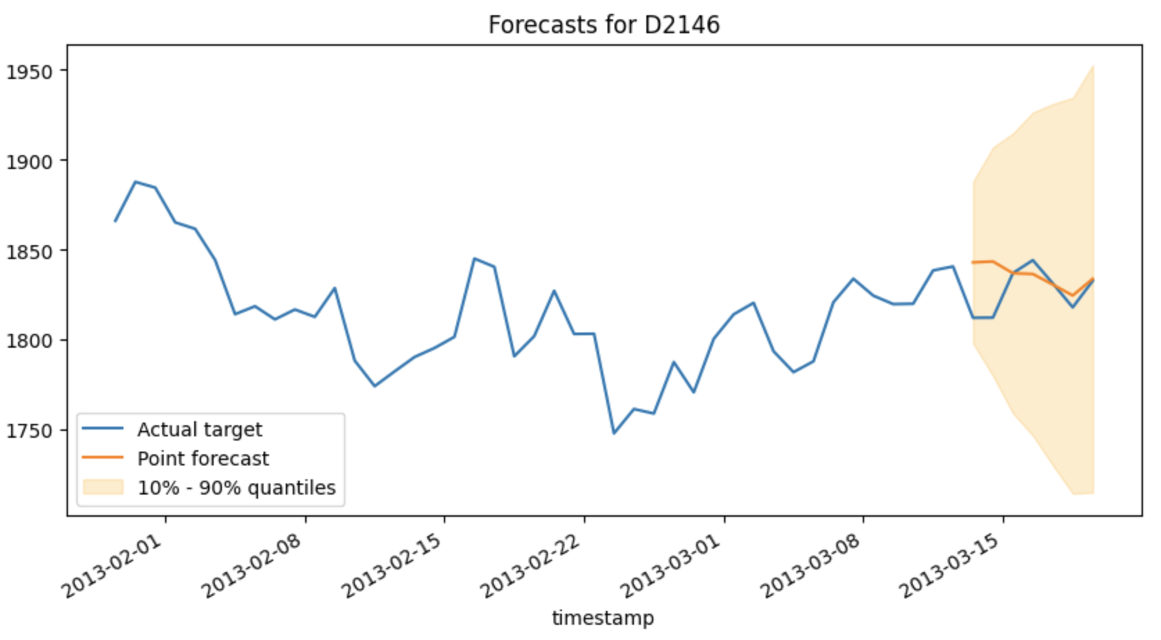
By default, AutoGluon-TimeSeries provides both point forecasts and probabilistic (quantile) forecasts of the target value. Probabilistic forecasts are essential in many planning tasks, and they can be used to flexibly compute intervals, enabling downstream tasks such as inventory and capacity planning.

The following is a sample forecast plot demonstrating point forecasts and prediction intervals.

Conclusion

AutoGluon-TimeSeries gives forecasters and data scientists a quick and easy way to build powerful forecasting models. In addition to some of the library’s commonly used features showcased in this post, AutoGluon-TimeSeries features a set of ways to configure forecasts for advanced users. Predictors are also easy to train, deploy, and serve at scale with Amazon SageMaker, using AutoGluon deep learning containers.

For more details on using AutoGluon, examples, tutorials, as well as other tasks AutoGluon tackles such as learning on tabular or multimodal data, visit AutoGluon. To get started using AutoGluon-TimeSeries, check out our quick start tutorial or our in-depth tutorial for a deeper look into all features the library offers. Follow AutoGluon on Twitter, and star us on GitHub to be informed of the latest updates.

For forecasting at scale with dedicated compute and workflows, enterprise-level support, forecast explainability and more, also check out Amazon Forecast.

References

[1] Salinas, David, Valentin Flunkert, Jan Gasthaus, and Tim Januschowski. “DeepAR: Probabilistic forecasting with autoregressive recurrent networks.” International Journal of Forecasting 36. 3 (2020): 1181-1191.

[2] Lim, Bryan, Sercan O Arik, Nicolas Loeff, and Tomas Pfister. “Temporal Fusion Transformers for interpretable multi-horizon time series forecasting.” International Journal of Forecasting 37.4 (2021): 1748-1764.

[3] Makridakis, Spyros, Evangelos Spiliotis, and Vassilios Assimakopoulos. “The M4 Competition: 100,000 time series and 61 forecasting methods.” International Journal of Forecasting 36.1 (2020): 54-74.


About the authors

Caner Turkmen is an Applied Scientist at Amazon Web Services, where he works on problems at the intersection of machine learning and forecasting, in addition to developing AutoGluon-TimeSeries. Before joining AWS, he worked in the management consulting industry as a data scientist, serving the financial services and telecommunications industries on projects across the globe. Caner’s personal research interests span a range of topics, including forecasting, causal inference, and AutoML.

Oleksandr Shchur is an Applied Scientist at Amazon Web Services, where he works on time series forecasting in AutoGluon-TimeSeries. Before joining AWS, he completed a PhD in Machine Learning at the Technical University of Munich, Germany, doing research on probabilistic models for event data. His research interests include machine learning for temporal data and generative modeling.

Nick Erickson is a Senior Applied Scientist at Amazon Web Services. He obtained his master’s degree in Computer Science and Engineering from the University of Minnesota Twin Cities. He is the co-author and lead developer of the open-source AutoML framework AutoGluon. Starting as a personal competition ML toolkit in 2018, Nick continually expanded the capabilities of AutoGluon and joined Amazon AI in 2019 to open-source the project and work full time on advancing the state-of-the-art in AutoML.

Read More

Conversation Summaries in Google Chat

Conversation Summaries in Google Chat

Information overload is a significant challenge for many organizations and individuals today. It can be overwhelming to keep up with incoming chat messages and documents that arrive at our inbox everyday. This has been exacerbated by the increase in virtual work and remains a challenge as many teams transition to a hybrid work environment with a mix of those working both virtually and in an office. One solution that can address information overload is summarization — for example, to help users improve their productivity and better manage so much information, we recently introduced auto-generated summaries in Google Docs.

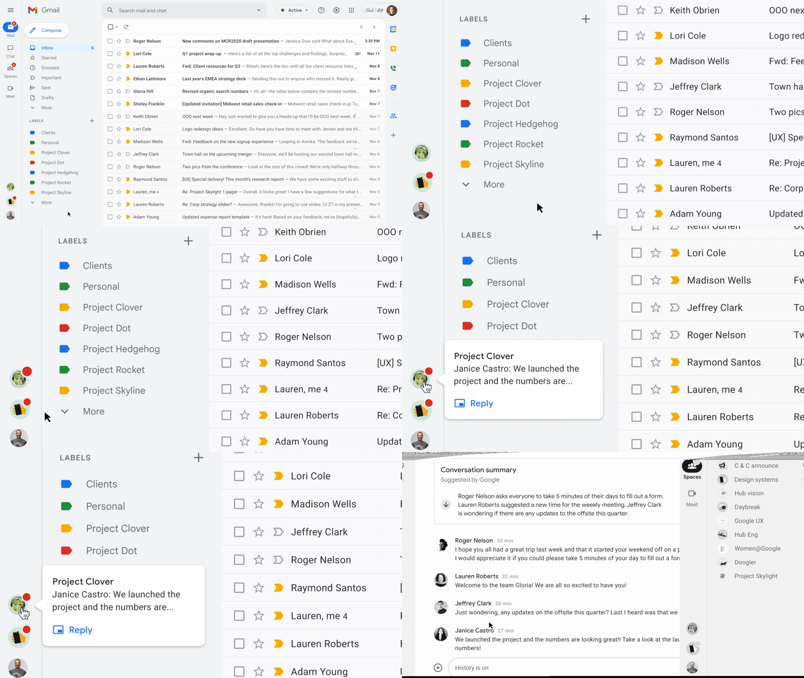
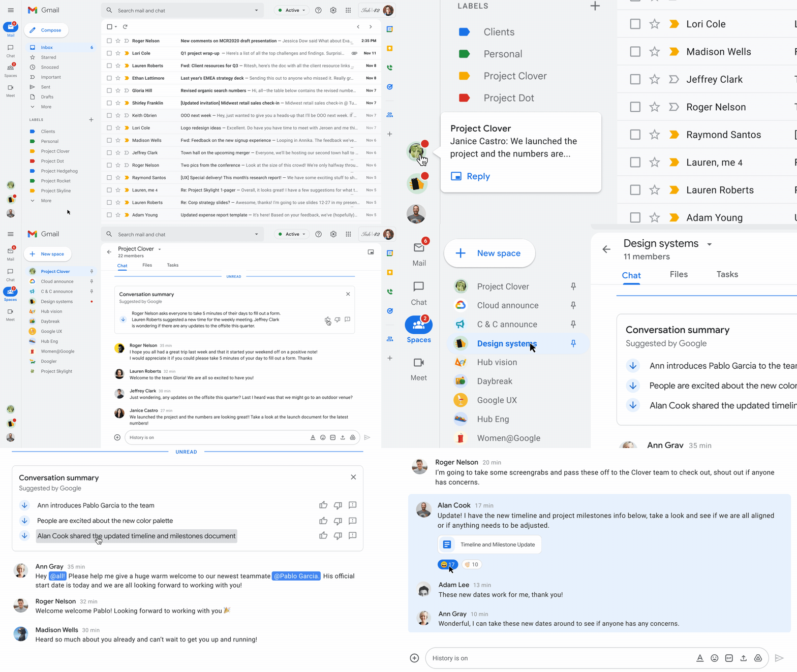
Today, we are excited to introduce conversation summaries in Google Chat for messages in Spaces. When these summaries are available, a card with automatically generated summaries is shown as users enter Spaces with unread messages. The card includes a list of summaries for the different topics discussed in Spaces. This feature is enabled by our state-of-the-art abstractive summarization model, Pegasus, which generates useful and concise summaries for chat conversations, and is currently available to selected premium Google Workspace business customers.

Conversation summaries provide a helpful digest of conversations in Spaces, allowing users to quickly catch-up on unread messages and navigate to the most relevant threads.

Conversation Summarization Modeling

The goal of text summarization is to provide helpful and concise summaries for different types of text, such as documents, articles, or spoken conversations. A good summary covers the key points succinctly, and is fluent and grammatically correct. One approach to summarization is to extract key parts from the text and concatenate them together into a summary (i.e., extractive summarization). Another approach is to use natural language generation (NLG) techniques to summarize using novel words and phrases not necessarily present in the original text. This is referred to as abstractive summarization and is considered closer to how a person would generally summarize text. A main challenge with abstractive summarization, however, is that it sometimes struggles to generate accurate and grammatically correct summaries, especially in real world applications.

ForumSum Dataset

The majority of abstractive summarization datasets and research focuses on single-speaker text documents, like news and scientific articles, mainly due to the abundance of human-written summaries for such documents. On the other hand, datasets of human-written summaries for other types of text, like chat or multi-speaker conversations, are very limited.

To address this we created ForumSum, a diverse and high-quality conversation summarization dataset with human-written summaries. The conversations in the dataset are collected from a wide variety of public internet forums, and are cleaned up and filtered to ensure high quality and safe content (more details in the paper).

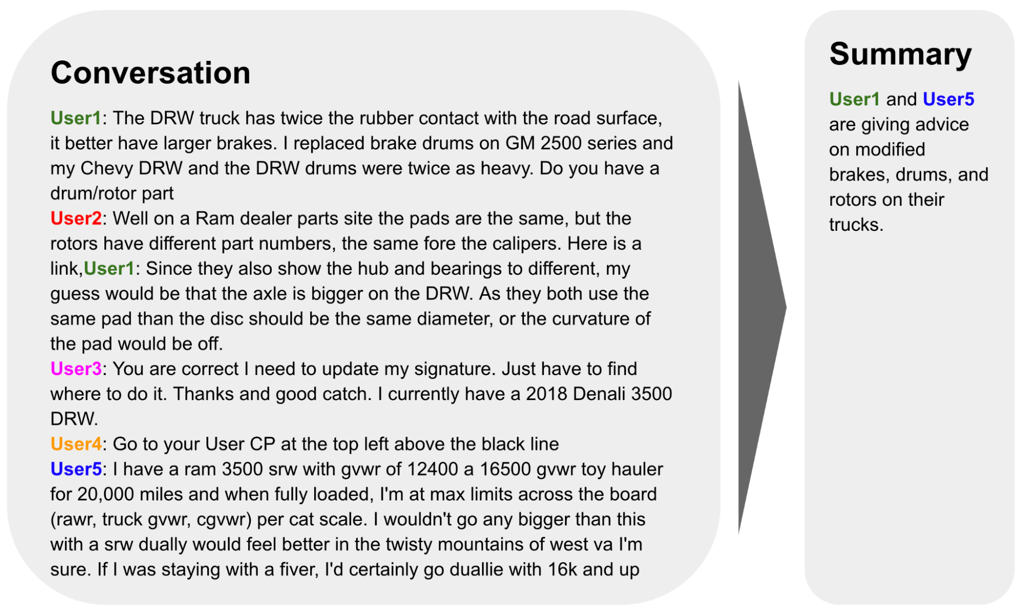
An example from the ForumSum dataset.

Each utterance in the conversation starts on a new line, contains an author name and a message text that is separated with a colon. Human annotators are then given detailed instructions to write a 1-3 sentence summary of the conversation. These instructions went through multiple iterations to ensure annotators wrote high quality summaries. We have collected summaries for over six thousand conversations, with an average of more than 6 speakers and 10 utterances per conversation. ForumSum provides quality training data for the conversation summarization problem: it has a variety of topics, number of speakers, and number of utterances commonly encountered in a chat application.

Conversation Summarization Model Design

As we have written previously, the Transformer is a popular model architecture for sequence-to-sequence tasks, like abstractive summarization, where the inputs are the document words and the outputs are the summary words. Pegasus combined transformers with self-supervised pre-training customized for abstractive summarization, making it a great model choice for conversation summarization. First, we fine-tune Pegasus on the ForumSum dataset where the input is the conversation words and the output is the summary words. Second, we use knowledge distillation to distill the Pegasus model into a hybrid architecture of a transformer encoder and a recurrent neural network (RNN) decoder. The resulting model has lower latency and memory footprint while maintaining similar quality as the Pegasus model.

Quality and User Experience

A good summary captures the essence of the conversation while being fluent and grammatically correct. Based on human evaluation and user feedback, we learned that the summarization model generates useful and accurate summaries most of the time. But occasionally the model generates low quality summaries. After looking into issues reported by users, we found that there are two main types of low quality summaries. The first one is misattribution, when the model confuses which person or entity said or performed a certain action. The second one is misrepresentation, when the model’s generated summary misrepresents or contradicts the chat conversation.

To address low quality summaries and improve the user experience, we have made progress in several areas:

  1. Improving ForumSum: While ForumSum provides a good representation of chat conversations, we noticed certain patterns and language styles in Google Chat conversations that differ from ForumSum, e.g., how users mention other users and the use of abbreviations and special symbols. After exploring examples reported by users, we concluded that these out-of-distribution language patterns contributed to low quality summaries. To address this, we first performed data formatting and clean-ups to reduce mismatches between chat and ForumSum conversations whenever possible. Second, we added more training data to ForumSum to better represent these style mismatches. Collectively, these changes resulted in reduction of low quality summaries.
  2. Controlled triggering: To make sure summaries bring the most value to our users, we first need to make sure that the chat conversation is worthy of summarization. For example, we found that there is less value in generating a summary when the user is actively engaged in a conversation and does not have many unread messages, or when the conversation is too short.
  3. Detecting low quality summaries: While the two methods above limited low quality and low value summaries, we still developed methods to detect and abstain from showing such summaries to the user when they are generated. These are a set of heuristics and models to measure the overall quality of summaries and whether they suffer from misattribution or misrepresentation issues.

Finally, while the hybrid model provided significant performance improvements, the latency to generate summaries was still noticeable to users when they opened Spaces with unread messages. To address this issue, we instead generate and update summaries whenever there is a new message sent, edited or deleted. Then summaries are cached ephemerally to ensure they surface smoothly when users open Spaces with unread messages.

Conclusion and Future Work

We are excited to apply state-of-the-art abstractive summarization models to help our Workspace users improve their productivity in Spaces. While this is great progress, we believe there are many opportunities to further improve the experience and the overall quality of summaries. Future directions we are exploring include better modeling and summarizing entangled conversations that include multiple topics, and developing metrics that better measure the factual consistency between chat conversations and summaries.

Acknowledgements

The authors would like to thank the many people across Google that contributed to this work: Ahmed Chowdhury, Alejandro Elizondo, Anmol Tukrel, Benjamin Lee, Chao Wang, Chris Carroll, Don Kim, Jackie Tsay, Jennifer Chou, Jesse Sliter, John Sipple, Kate Montgomery, Maalika Manoharan, Mahdis Mahdieh, Mia Chen, Misha Khalman, Peter Liu, Robert Diersing, Sarah Read, Winnie Yeung, Yao Zhao, and Yonghui Wu.

Read More

Your guide to AI/ML at AWS re:Invent 2022

Your guide to AI/ML at AWS re:Invent 2022

AWS re:Invent season is upon us again! Just a few days to go until re:Invent takes place for the 11th year in Las Vegas, Nevada. The Artificial Intelligence and Machine Learning team at AWS has been working hard to offer amazing content, an outstanding AWS DeepRacer experience, and much more. In this post, we give you a sense of how the AI/ML track is organized and highlight a few sessions we think you’ll like.

The technical sessions in the AI/ML track are divided into four areas. First, there are many common use cases that you can address with a combination of AI/ML and other AWS services, such as Intelligent Document Processing, Contact Center Intelligence, and Personalization among others. Second, ML practitioners of all levels will find compelling content on the entire ML lifecycle, such as data preparation, training, inference, MLOps, AutoML, and no-code ML. This year, we have a renewed emphasis on responsible AI. Customers have been looking for more guidance and new tools in this space. And last but never least, we have exciting workshops and activities with AWS DeepRacer—they have become a signature event!

Visit the AWS Village at the Venetian Expo Hall to meet our AI/ML specialists at the AI/ML booth and learn more about AI/ML services and solutions. You can also chat with our AWS Manufacturing experts at the AWS Industries Networking Lounge, in the Caesars Forum Main Hall.

If you’re new to re:Invent, you can attend sessions of the following types:

  • Keynotes – Join in-person or virtual, and learn about all the exciting announcements.
  • Leadership sessions – Learn from AWS leaders about key topics in cloud computing.
  • Breakout sessions – These 60-minute sessions are expected to have broad appeal, are delivered to larger audiences, and will be recorded. If you miss them, you can watch them on demand after re:Invent.
  • Chalk talks – 60 minutes of content delivered to smaller audiences with an interactive whiteboarding session. Chalk talks are where discussions happen, and these offer you the greatest opportunity to ask questions or share your opinion.
  • Workshops – Hands-on learning opportunities where, in the course of 2 hours, you’ll be able to build a solution to a problem, understand the inner workings of the resulting infrastructure, and cross-service interaction. Bring your laptop and be ready to learn!
  • Builders’ sessions – These highly interactive 60-minute mini-workshops are conducted in small groups of less than 10 attendees. Some of these appeal to beginners, and others are on specialized topics.

If you have reserved your seat at any of the sessions, great! If not, we always set aside some spots for walk-ins, so make a plan and come to the room early.

To help you plan your agenda for this year’s re:Invent, here are some highlights of the AI/ML track. So buckle up, and start registering for your favorite sessions.

Visit the session catalog to learn about all AI/ML sessions.

AWS Data and Machine Learning Keynote

Swami Sivasubramanian, Vice President of AWS Data and Machine Learning – Keynote

Wednesday November 30 | 8:30 AM – 10:30 AM PST | The Venetian

Join Swami Sivasubramanian, Vice President of AWS Data and Machine Learning on Wednesday, as he reveals the latest AWS innovations that can help you transform your company’s data into meaningful insights and actions for your business, in person or via livestream.

AI/ML Leadership session

AIM217-L (LVL 200) Innovate with AI/ML to transform your business

Wednesday November 30 | 1:00 PM – 2:00 PM PST

Join Dr. Bratin Saha, VP of AI/ML at AWS, for the AI/ML thought-leadership session. Bratin will share how to use AI/ML to innovate in your business in order to disrupt the status quo. You learn how customers Baxter, BMW, and Alexa have used AWS AI/ML services to fuel business profitability and growth, the latest AI/ML trends, and the details of newly launched AWS capabilities.

Reserve your seat now!

Breakout sessions

AIM314 (LVL 300) Accelerate your ML journey with Amazon SageMaker low-code tools

Monday November 28 | 10:00 AM – 11:00 AM PST

In this session, learn how low-code tools, including Amazon SageMaker Data Wrangler, Amazon SageMaker Autopilot, and Amazon SageMaker JumpStart, make it easier to experiment faster and bring highly accurate models to production more quickly and efficiently.

Reserve your seat now!

AIM204 (LVL 200) Automate insurance document processing with AI

Monday November 28 | 4:00 PM – 5:00 PM PST

The rapid rate of data generation means that organizations that aren’t investing in document automation risk getting stuck with legacy processes that are slow, error-prone, and difficult to scale. In this session, learn how organizations can take advantage of the latest innovations in AI and ML from AWS to improve the efficiency of their document-intensive claims processing use case.

Reserve your seat now!

AIM207 (LVL 200) Make better decisions with no-code ML using SageMaker Canvas, feat. Samsung

Wednesday November 30 | 2:30 PM – 3:30 PM PSTOrganizations everywhere use ML to accurately predict outcomes and make faster business decisions. In this session, learn how you can use Amazon SageMaker Canvas to access and combine data from a variety of sources, clean data, build ML models to generate predictions with a single click, and share models across your organization to improve productivity.

Reserve your seat now!

AIM307 (LVL 300) JPMorganChase real-time agent assist for contact center productivity

Wednesday November 30 | 11:30 AM – 12:30 PM PST

Resolving complex customer issues is often time-consuming and requires agents to quickly gather relevant information from knowledge bases to resolve queries accurately. Join this session to learn how JPMorgan Chase built an AWS Contact Center Intelligence (CCI) real-time agent assist solution to help 75 million customers and help 8,500 servicing agents generate next best actions in the shortest time—reducing agent frustration and churn.

Reserve your seat now!

AIM321 (LVL 300) Productionize ML workloads using Amazon SageMaker MLOps, feat. NatWest

Wednesday November 30 | 4:45 PM – 5:45 PM PST

Amazon SageMaker provides a breadth of MLOps tools to train, test, troubleshoot, deploy, and govern ML models at scale. In this session, explore SageMaker MLOps features, including SageMaker Pipelines, SageMaker Projects, SageMaker Experiments, SageMaker Model Registry, and SageMaker Model Monitor, and learn how to increase automation and improve the quality of your ML workflows.

Reserve your seat now!

AIM319 (LVL 300) Build, manage, and scale ML development with a web-based visual interface

Wednesday November 30 | 3:15 PM – 4:15 PM PST

Amazon SageMaker Studio is an integrated development environment (IDE) for data science and ML. In this session, explore how to use SageMakerStudio to prepare data and build, train, deploy, and manage ML models from a single, web-based visual interface.

Reserve your seat now!

Chalk talks

AIM341-R (LVL 300) Transforming responsible AI from theory into practice

Thursday December 1 | 4:15 PM – 5:15 PM PST

The practices of responsible AI can help reduce biased outcomes from models and improve their fairness, explainability, robustness, privacy, and transparency. Walk away from this chalk talk with best practices and hands-on support to guide you in applying responsible AI in your project.

Reserve your seat now!

*This chalk talk will be repeated Wednesday November 30 | 7:00 PM – 8:00 PM PST

AIM306-R (LVL 300) Automate content moderation and compliance with AI

Monday November 28 | 12:15 PM – 1:15 PM PST

In this chalk talk, learn how to efficiently moderate high volumes of user-generated content across media types with AI. Discover how to add humans in the moderation loop to verify low-confidence decisions and continuously improve ML models to keep online communities safe and inclusive and lower content moderation costs.

Reserve your seat now!

*This chalk talk will be repeated Wednesday November 30 | 9:15 AM – 10:15 AM PST

AIM407-R (LVL 400) Choosing the right ML instance for training and inference on AWS

Wednesday November 30 | 11:30 AM – 12:30 PM PST

This chalk talk guides you through how to choose the right compute instance type on AWS for your deep learning projects. Explore the available options, such as the most performant instance for training, the best instance for prototyping, and the most cost-effective instance for inference deployments.

Reserve your seat now!

*This chalk talk will be repeated Wednesday November 30 | 8:30 AM – 9:30 AM PST

AIM328-R (LVL 300) Explain your ML models with Amazon SageMaker Clarify

Tuesday November 29 | 2:00 PM – 3:00 PM PST

Amazon SageMaker Clarify helps organizations understand their model predictions by providing real-time explanations for models deployed on SageMaker endpoints. In this chalk talk, learn how to identify the importance of various features in overall model predictions and for individual inferences using Shapley values and detect any shifts in feature importance over time after a model is deployed to production.

Reserve your seat now!

*This chalk talk will be repeated Monday November 28 | 2:30 PM – 3:30 PM PST

Workshops

AIM342 (LVL 300) Advancing responsible AI: Bias assessment and transparency

Wednesday November 30 | 2:30 PM – 4:30 PM PST

Building and operating ML applications responsibly requires an active, consistent approach to prevent, assess, and mitigate bias. This workshop takes you through a computer vision case study in assessing unwanted bias—follow along during the workshop with a Jupyter notebook.

Reserve your seat now!

AIM402-R (LVL 400) Extract AI-driven customer insights using Post-Call Analytics

Monday November 28 | 4:00 PM – 6:00 PM PST

Companies are transforming existing contact centers by adding AI/ML to deliver actionable insights and improve automation with existing telephony systems. Join this workshop to learn how to use the AWS Contact Center Intelligence (CCI) Post-Call Analytics solution to derive AI-driven insights from virtually all customer conversations.

Reserve your seat now!

*This workshop will be repeated Wednesday November 30 | 9:15 AM – 11:15 AM PST

AIM212-R (LVL 200) Deep learning with Amazon SageMaker, AWS Trainium, and AWS Inferentia

Monday November 28 | 1:00 PM – 3:00 PM PST

Amazon EC2 Trn1 instances, powered by AWS Trainium, and Amazon EC2 Inf1 instances, powered by AWS Inferentia, deliver the best price performance for deep learning training and inference. In this workshop, walk through training a BERT model for natural language processing on Trn1 instances to save up to 50% in training costs over equivalent GPU-based EC2 instances.

Reserve your seat now!

*This workshop will be repeated Monday November 28 | 8:30 AM – 10:30 AM PST

AIM312-R (LVL 300) Build a custom recommendation engine in 2 hours with Amazon Personalize

Monday November 28 | 1:00 PM – 3:00 PM PST

In this workshop, learn how to build a customer-specific solution using your own data to deliver personalized experiences that can be integrated into your existing websites, applications, SMS, and email marketing systems using simple APIs.

Reserve your seat now!

*This workshop will be repeated Wednesday November 30 | 11:30 AM – 1:30 PM PST

Builders’ sessions

AIM325-R (LVL 300) Build applications faster with an ML-powered coding companion

Tuesday November 29 | 3:30 PM – 4:30 PM PST

Join this builders’ session to get hands-on experience with ML-powered developer tools from AWS. Learn how to accelerate application development with automatic code recommendations from Amazon CodeWhisperer and automate code reviews with Amazon CodeGuru.

Reserve your seat now!

*This session will be repeated Thursday December 1 | 12:30 PM – 1:30 PM PST

Make sure to check out the re:Invent content catalog or the AI/ML attendee guide for more AI/ML content at re:Invent.

AWS DeepRacer: Get hands-on with machine learning

Developers of all skill levels can get hands-on with ML at re:Invent by participating in AWS DeepRacer. Learn to build your own ML model from AWS ML experts in one of 11 workshop sessions, featuring guest speakers from JPMorgan Chase and Intel. Compete by racing your own ML model on real championship tracks in both the MGM and the Sands Expo, or hop in the driver’s seat to experience ML fundamentals through the fun of gamified learning with AWS DeepRacer Arcades. Whether in the classroom, on the track, or behind the wheel, AWS DeepRacer is the fastest way to get rolling with ML.

Developers: start your engines! Starting Monday November 28, the top 50 racers from around the world compete in the AWS DeepRacer League Championships presented by Intel, hosted at the AWS DeepRacer Championship Stadium in the Sands Expo. Watch trackside or tune in live on twitch.tv/aws at 3:00 PM PST on Tuesday, November 29, to see the top eight racers battle it out in the semifinals. Cheer on the finalists as they go for their shot at $20,000 in cash prizes and the right to hoist the Championship Cup.

Race on any AWS DeepRacer track on Thursday, December 1, to compete in the 2023 re:Invent Open, where the fastest competitor of the day will claim an all-expenses paid trip back to Vegas to compete in the 2023 AWS DeepRacer Championship Cup.

Attendees who participate in AWS DeepRacer Arcades or open track (non-competitive) racing will also have the chance to win one of six spots in the AWS DeepRacer Winner’s Circle Driving Experience Sweepstakes, where they will race real, full-size exotic cars on a closed track alongside the AWS DeepRacer 2022 Champions in Las Vegas.

Don’t forget to check out the AWS DeepRacer workshops before they fill up to reserve your spot. We can’t wait to see you in Las Vegas!


About the authors

Denis V. Batalov is a 17-year Amazon veteran and a PhD in Machine Learning, Denis worked on such exciting projects as Search Inside the Book, Amazon Mobile apps and Kindle Direct Publishing. Since 2013 he has helped AWS customers adopt AI/ML technology as a Solutions Architect. Currently, Denis is a Worldwide Tech Leader for AI/ML responsible for the functioning of AWS ML Specialist Solutions Architects globally. Denis is a frequent public speaker, you can follow him on Twitter @dbatalov.

Amelie Perkuhn is a Product Marketing Manager on the AI Services team at AWS. She has held various roles within AWS over the past 6 years, and in her current role, she is focused on driving adoption of AI Services including Amazon Kendra. In her spare time, Amelie enjoys the Pacific Northwest with her dog Moxie.

Read More