EHR-Safe: Generating High-Fidelity and Privacy-Preserving Synthetic Electronic Health Records

EHR-Safe: Generating High-Fidelity and Privacy-Preserving Synthetic Electronic Health Records

Analysis of Electronic Health Records (EHR) has a tremendous potential for enhancing patient care, quantitatively measuring performance of clinical practices, and facilitating clinical research. Statistical estimation and machine learning (ML) models trained on EHR data can be used to predict the probability of various diseases (such as diabetes), track patient wellness, and predict how patients respond to specific drugs. For such models, researchers and practitioners need access to EHR data. However, it can be challenging to leverage EHR data while ensuring data privacy and conforming to patient confidentiality regulations (such as HIPAA).

Conventional methods to anonymize data (e.g., de-identification) are often tedious and costly. Moreover, they can distort important features from the original dataset, decreasing the utility of the data significantly; they can also be susceptible to privacy attacks. Alternatively, an approach based on generating synthetic data can maintain both important dataset features and privacy.

To that end, we propose a novel generative modeling framework in “EHR-Safe: Generating High-Fidelity and Privacy-Preserving Synthetic Electronic Health Records“. With the innovative methodology in EHR-Safe, we show that synthetic data can satisfy two key properties: (i) high fidelity (i.e., they are useful for the task of interest, such as having similar downstream performance when a diagnostic model is trained on them), (ii) meet certain privacy measures (i.e., they do not reveal any real patient’s identity). Our state-of-the-art results stem from novel approaches for encoding/decoding features, normalizing complex distributions, conditioning adversarial training, and representing missing data.

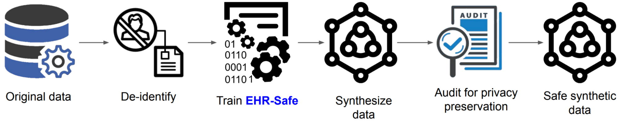
Generating synthetic data from the original data with EHR-Safe.

Challenges of Generating Realistic Synthetic EHR Data

There are multiple fundamental challenges to generating synthetic EHR data. EHR data contain heterogeneous features with different characteristics and distributions. There can be numerical features (e.g., blood pressure) and categorical features with many or two categories (e.g., medical codes, mortality outcome). Some of these may be static (i.e., not varying during the modeling window), while others are time-varying, such as regular or sporadic lab measurements. Distributions might come from different families — categorical distributions can be highly non-uniform (e.g., for under-represented groups) and numerical distributions can be highly skewed (e.g., a small proportion of values being very large while the vast majority are small). Depending on a patient’s condition, the number of visits can also vary drastically — some patients visit a clinic only once whereas some visit hundreds of times, leading to a variance in sequence lengths that is typically much higher compared to other time-series data. There can be a high ratio of missing features across different patients and time steps, as not all lab measurements or other input data are collected.

Examples of real EHR data: temporal numerical features (upper) and temporal categorical features (lower).

EHR-Safe: Synthetic EHR Data Generation Framework

EHR-Safe consists of sequential encoder-decoder architecture and generative adversarial networks (GANs), depicted in the figure below. Because EHR data are heterogeneous (as described above), direct modeling of raw EHR data is challenging for GANs. To circumvent this, we propose utilizing a sequential encoder-decoder architecture, to learn the mapping from the raw EHR data to the latent representations, and vice versa.

Block diagram of EHR-Safe framework.

While learning the mapping, esoteric distributions of numerical and categorical features pose a great challenge. For example, some values or numerical ranges might dominate the distribution, but the capability of modeling rare cases is essential. The proposed feature mapping and stochastic normalization (transforming original feature distributions into uniform distributions without information loss) are key to handling such data by converting to distributions for which the training of encoder-decoder and GAN are more stable (details can be found in the paper). The mapped latent representations, generated by the encoder, are then used for GAN training. After training both the encoder-decoder framework and GANs, EHR-Safe can generate synthetic heterogeneous EHR data from any input, for which we feed randomly sampled vectors. Note that only the trained generator and decoders are used for generating synthetic data.

Datasets

We focus on two real-world EHR datasets to showcase the EHR-Safe framework, MIMIC-III and eICU. Both are inpatient datasets that consist of varying lengths of sequences and include multiple numerical and categorical features with missing components.

Fidelity Results

The fidelity metrics focus on the quality of synthetically generated data by measuring the realisticness of the synthetic data. Higher fidelity implies that it is more difficult to differentiate between synthetic and real data. We evaluate the fidelity of synthetic data in terms of multiple quantitative and qualitative analyses.

Visualization

Having similar coverage and avoiding under-representation of certain data regimes are both important for synthetic data generation. As the below t-SNE analyses show, the coverage of the synthetic data (blue) is very similar with the original data (red). With membership inference metrics (will be introduced in the privacy section), we also verify that EHR-Safe does not just memorize the original train data.

t-SNE analyses on temporal and static data on MIMIC-III (upper) and eICU (lower) datasets.

Statistical Similarity

We provide quantitative comparisons of statistical similarity between original and synthetic data for each feature. Most statistics are well-aligned between original and synthetic data — for example a measure of the KS statistics, i.e,. the maximum difference in the cumulative distribution function (CDF) between the original and the synthetic data, are mostly lower than 0.03. More detailed tables can be found in the paper. The figure below exemplifies the CDF graphs for original vs. synthetic data for three features — overall they seem very close in most cases.

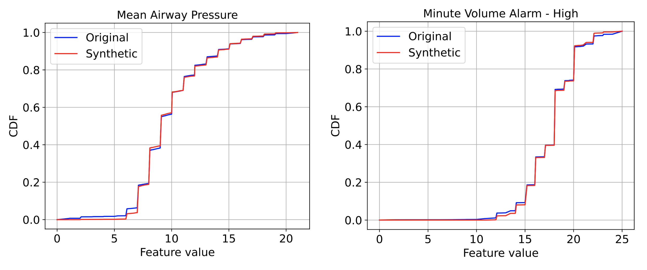
CDF graphs of two features between original and synthetic EHR data. Left: Mean Airway Pressure. Right: Minute Volume Alarm.

Utility

Because one of the most important use cases of synthetic data is enabling ML innovations, we focus on the fidelity metric that measures the ability of models trained on synthetic data to make accurate predictions on real data. We compare such model performance to an equivalent model trained with real data. Similar model performance would indicate that the synthetic data captures the relevant informative content for the task. As one of the important potential use cases of EHR, we focus on the mortality prediction task. We consider four different predictive models: Gradient Boosting Tree Ensemble (GBDT), Random Forest (RF), Logistic Regression (LR), Gated Recurrent Units (GRU).

Mortality prediction performance with the model trained on real vs. synthetic data. Left: MIMIC-III. Right: eICU.

In the figure above we see that in most scenarios, training on synthetic vs. real data are highly similar in terms of Area Under Receiver Operating Characteristics Curve (AUC). On MIMIC-III, the best model (GBDT) on synthetic data is only 2.6% worse than the best model on real data; whereas on eICU, the best model (RF) on synthetic data is only 0.9% worse.

Privacy Results

We consider three different privacy attacks to quantify the robustness of the synthetic data with respect to privacy.

  • Membership inference attack: An adversary predicts whether a known subject was a present in the training data used for training the synthetic data model.
  • Re-identification attack: The adversary explores the probability of some features being re-identified using synthetic data and matching to the training data.
  • Attribute inference attack: The adversary predicts the value of sensitive features using synthetic data.
Privacy risk evaluation across three privacy metrics: membership-inference (top-left), re-identification (top-right), and attribute inference (bottom). The ideal value of privacy risk for membership inference is random guessing (0.5). For re-identification, the ideal case is to replace the synthetic data with disjoint holdout original data.

The figure above summarizes the results along with the ideal achievable value for each metric. We observe that the privacy metrics are very close to the ideal in all cases. The risk of understanding whether a sample of the original data is a member used for training the model is very close to random guessing; it also verifies that EHR-Safe does not just memorize the original train data. For the attribute inference attack, we focus on the prediction task of inferring specific attributes (e.g., gender, religion, and marital status) from other attributes. We compare prediction accuracy when training a classifier with real data against the same classifier trained with synthetic data. Because the EHR-Safe bars are all lower, the results demonstrate that access to synthetic data does not lead to higher prediction performance on specific features as compared to access to the original data.

Comparison to Alternative Methods

We compare EHR-Safe to alternatives (TimeGAN, RC-GAN, C-RNN-GAN) proposed for time-series synthetic data generation. As shown below, EHR-Safe significantly outperforms each.

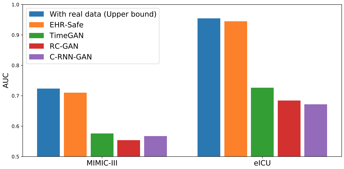
Downstream task performance (AUC) in comparison to alternatives.

Conclusions

We propose a novel generative modeling framework, EHR-Safe, that can generate highly realistic synthetic EHR data that are robust to privacy attacks. EHR-Safe is based on generative adversarial networks applied to the encoded raw data. We introduce multiple innovations in the architecture and training mechanisms that are motivated by the key challenges of EHR data. These innovations are key to our results that show almost-identical properties with real data (when desired downstream capabilities are considered) with almost-ideal privacy preservation. An important future direction is generative modeling capability for multimodal data, including text and image, as modern EHR data might contain both.

Acknowledgements

We gratefully acknowledge the contributions of Michel Mizrahi, Nahid Farhady Ghalaty, Thomas Jarvinen, Ashwin S. Ravi, Peter Brune, Fanyu Kong, Dave Anderson, George Lee, Arie Meir, Farhana Bandukwala, Elli Kanal, and Tomas Pfister.

Read More

Announcing the updated Salesforce connector (V2) for Amazon Kendra

Announcing the updated Salesforce connector (V2) for Amazon Kendra

Amazon Kendra is a highly accurate and simple-to-use intelligent search service powered by machine learning (ML). Amazon Kendra offers a suite of data source connectors to simplify the process of ingesting and indexing your content, wherever it resides.

Valuable data in organizations is stored in both structured and unstructured repositories. An enterprise search solution should be able to pull together data across several structured and unstructured repositories to index and search on.

One such data repository is Salesforce. Salesforce is a comprehensive CRM tool for managing support, sales, and marketing teams. It’s an intelligent, proactive, AI-powered platform that empowers employees with the information they need to make the best decisions for every customer. It’s the backbone of the world’s most customer-centered organizations and helps companies put the customer at the center of everything they do.

We’re excited to announce that we have updated the Salesforce connector for Amazon Kendra to add even more capabilities. In this version (V2), we have added support for Salesforce Lightning in addition to Classic. You can now choose to crawl attachments and also bring in identity/ACL information to make your searches more granular. We now support 20 standard entities, and you can choose to index more fields.

You can import the following entities (and attachments for those marked with *):

  • Accounts*
  • Campaign*
  • Partner
  • Pricebook
  • Case*
  • Contact*
  • Contract*
  • Document
  • Group
  • Idea
  • Lead*
  • Opportunity*
  • Product
  • Profile
  • Solution*
  • Task*
  • User*
  • Chatter*
  • Knowledge Articles
  • Custom Objects*

Solution overview

With Amazon Kendra, you can configure multiple data sources to provide a central place to search across your document repository. For our solution, we demonstrate how to index a Salesforce repository or folder using the Amazon Kendra connector for Salesforce. The solution consists of the following steps:

  1. Create and configure an app on Salesforce and get the connection details.
  2. Create a Salesforce data source via the Amazon Kendra console.
  3. Index the data in the Salesforce repository.
  4. Run a sample query to get the information.
  5. Filter the query by users or groups.

Prerequisites

To try out the Amazon Kendra connector for Salesforce, you need the following:

Configure a Salesforce app and gather connection details

Before we set up the Salesforce data source, we need a few details about your Salesforce repository. Let’s gather those in advance (refer to Authorization Through Connected Apps and OAuth 2.0 for more details).

  1. Go to https://login.salesforce.com/ and log in with your credentials.

  2. In the navigation pane, choose Setup Home.
  3. Under Apps, choose App Manager.

    This refreshes the right pane.

  4. Choose New Connected App.

  5. Select Enable OAuth Settings to expand the API (Enable OAuth Settings) section.
  6. For Callback URL, enter https://login.salesforce.com/services/oauth2/token.
  7. For Selected OAuth Scopes, choose eclair_api and choose the right arrow icon.
  8. Select Introspect All Tokens.

  9. Choose Save.A warning appears that says “Changes can take up to 10 minutes to take effect.”
  10. Choose Continue to acknowledge.
  11. On the confirmation page, choose Manage Consumer Details.

  12. Copy and save the values for Consumer Key and Consumer Secret to use later when setting up your Amazon Kendra data source.

    Next, we generate a security token.

  13. On the home page, choose the View Profile icon and choose Settings.

  14. In the navigation pane, expand My Personal Information and choose Reset My Security Token.

    The security token is sent to the email you used when configuring the app. The following screenshot shows an example email.

  15. Save the security token to use when you configure the Salesforce connector to Amazon Kendra.

Configure the Amazon Kendra connector for Salesforce

To configure the Amazon Kendra connector, complete the following steps:

  1. On the Amazon Kendra console, choose Create an Index.

  2. For Index name, enter a name for the index (for example, my-salesforce-index).
  3. Enter an optional description.
  4. Choose Create a new role.
  5. For Role name, enter an IAM role name.
  6. Configure optional encryption settings and tags.
  7. Choose Next.

  8. In the Configure user access control section, leave the settings at their defaults and choose Next.

  9. Select Developer edition and choose Create.

    This creates and propagates the IAM role and then creates the Amazon Kendra index, which can take up to 30 minutes.

  10. Return to the Amazon Kendra console and choose Data sources in the navigation pane.

  11. Scroll down and locate Salesforce Online connector V2.0, and choose Add connector.

  12. For Data source name, enter a name (for example, my-salesforce-datasourcev2).
  13. Enter an optional description.
  14. Choose Next.

  15. For Salesforce URL, enter the URL at the top of the browser when you log in to Salesforce.
  16. For Configure VPC and security group, leave the default (No VPC).
  17. Keep Identity crawler is on selected.This imports identity/ACL information into the index.
  18. For IAM role, choose Create a new role.
  19. Enter a role name, such as AmazonKendra-salesforce-datasourcev2.
  20. Choose Next.

  21. In the Authentication section, choose Create and add new secret.

  22. Enter the details you gathered while setting up the Salesforce app:
    1. Secret name – The name you gave your secret.
    2. Username – The user name you use to log in to Salesforce.
    3. Password – The password you use to log in to Salesforce.
    4. Security token – The security token you received in your email while going through the setup in Salesforce.
    5. Consumer key – The key generated while going through the setup in Salesforce.
    6. Consumer secret – The secret generated while going through the setup in Salesforce.
    7. Authentication URL – Enter https://login.salesforce.com/services/oauth2/token.
  23. Choose Save.

    The next page is prefilled with the name of the secret.

  24. Choose Next.

  25. Select All standard objects and Include all attachments.
  26. For Sync run schedule, choose Run on demand.
  27. Choose Next.

  28. Keep all the defaults in the Field Mappings section and choose Next.
  29. On the review page, choose Add data source.

  30. Choose Sync now.

This indexes all the content in Salesforce as per your configuration. You will see a success message at the top of the page and also in the sync history.

Test the solution

Now that you have ingested the content from your Salesforce account into your Amazon Kendra index, you can test some queries.

  1. Go to your index and choose Search indexed content in the navigation pane.
  2. Enter a search term and press Enter.

    One of the features of the data source is that it brings in the ACL information along with the contents of Salesforce. You can use this to narrow down your queries by users or groups.

  3. Return to the search page and expand Test query with user name or groups.Choose Apply user name or groups.

  4. For Username, enter your user name and choose Apply.

    A message appears saying Attributes applied.

  5. Enter a new test query and press Enter.

Congratulations! You have successfully used Amazon Kendra to surface answers and insights based on the content indexed from your Salesforce account.

Conclusion

With the Salesforce connector for Amazon Kendra, organizations can tap into the repository of information stored in their account securely using intelligent search powered by Amazon Kendra.

In this post, we introduced you to the basics, but there are many additional features that we didn’t cover. For example:

  • You can enable user-based access control for your Amazon Kendra index and restrict access to users and groups that you configure
  • You can map additional fields to Amazon Kendra index attributes and enable them for faceting, search, and display in the search results
  • You can integrate the Salesforce data source with the Custom Document Enrichment (CDE) capability in Amazon Kendra to perform additional attribute mapping logic and even custom content transformation during ingestion

To learn about these possibilities and more, refer to the Amazon Kendra Developer Guide.


About the author

Ashish Lagwankar is a Senior Enterprise Solutions Architect at AWS. His core interests include AI/ML, serverless, and container technologies. Ashish is based in the Boston, MA, area and enjoys reading, outdoors, and spending time with his family.

Read More

­­Speed ML development using SageMaker Feature Store and Apache Iceberg offline store compaction

­­Speed ML development using SageMaker Feature Store and Apache Iceberg offline store compaction

Today, companies are establishing feature stores to provide a central repository to scale ML development across business units and data science teams. As feature data grows in size and complexity, data scientists need to be able to efficiently query these feature stores to extract datasets for experimentation, model training, and batch scoring.

Amazon SageMaker Feature Store is a purpose-built feature management solution that helps data scientists and ML engineers securely store, discover, and share curated data used in training and prediction workflows. SageMaker Feature Store now supports Apache Iceberg as a table format for storing features. This accelerates model development by enabling faster query performance when extracting ML training datasets, taking advantage of Iceberg table compaction. Depending on the design of your feature groups and their scale, you can experience training query performance improvements of 10x to 100x by using this new capability.

By the end of this post, you will know how to create feature groups using the Iceberg format, execute Iceberg’s table management procedures using Amazon Athena, and schedule these tasks to run autonomously. If you are a Spark user, you’ll also learn how to execute the same procedures using Spark and incorporate them into your own Spark environment and automation.

SageMaker Feature Store and Apache Iceberg

Amazon SageMaker Feature Store is a centralized store for features and associated metadata, allowing features to be easily discovered and reused by data scientist teams working on different projects or ML models.

SageMaker Feature Store consists of an online and an offline mode for managing features. The online store is used for low-latency real-time inference use cases. The offline store is primarily used for batch predictions and model training. The offline store is an append-only store and can be used to store and access historical feature data. With the offline store, users can store and serve features for exploration and batch scoring and extract point-in-time correct datasets for model training.

The offline store data is stored in an Amazon Simple Storage Service (Amazon S3) bucket in your AWS account. SageMaker Feature Store automatically builds an AWS Glue Data Catalog during feature group creation. Customers can also access offline store data using a Spark runtime and perform big data processing for ML feature analysis and feature engineering use cases.

Table formats provide a way to abstract data files as a table. Over the years, many table formats have emerged to support ACID transaction, governance, and catalog use cases. Apache Iceberg is an open table format for very large analytic datasets. It manages large collections of files as tables, and it supports modern analytical data lake operations such as record-level insert, update, delete, and time travel queries. Iceberg tracks individual data files in a table instead of in directories. This allows writers to create data files in place (files are not moved or changed) and only add files to the table in an explicit commit. The table state is maintained in metadata files. All changes to the table state create a new metadata file version that atomically replaces the older metadata. The table metadata file tracks the table schema, partitioning configuration, and other properties.

Iceberg has integrations with AWS services. For example, you can use the AWS Glue Data Catalog as the metastore for Iceberg tables, and Athena supports read, time travel, write, and DDL queries for Apache Iceberg tables that use the Apache Parquet format for data and the AWS Glue catalog for their metastore.

With SageMaker Feature Store, you can now create feature groups with Iceberg table format as an alternative to the default standard Glue format. With that, customers can leverage the new table format to use Iceberg’s file compaction and data pruning features to meet their use case and optimization requirements. Iceberg also lets customers perform deletion, time-travel queries, high-concurrency transactions, and higher-performance queries.

By combining Iceberg as a table format and table maintenance operations such as compaction, customers get faster query performance when working with offline feature groups at scale, letting them more quickly build ML training datasets.

The following diagram shows the structure of the offline store using Iceberg as a table format.

In the next sections, you will learn how to create feature groups using the Iceberg format, execute Iceberg’s table management procedures using AWS Athena and use AWS services to schedule these tasks to run on-demand or on a schedule. If you are a Spark user, you will also learn how to execute the same procedures using Spark.

For step-by-step instructions, we also provide a sample notebook, which can be found in GitHub. In this post, we will highlight the most important parts.

Creating feature groups using Iceberg table format

You first need to select Iceberg as a table format when creating new feature groups. A new optional parameter TableFormat can be set either interactively using Amazon SageMaker Studio or through code using the API or the SDK. This parameter accepts the values ICEBERG or GLUE (for the current AWS Glue format). The following code snippet shows you how to create a feature group using the Iceberg format and FeatureGroup.create API of the SageMaker SDK.

orders_feature_group_iceberg.create(
s3_uri=f"s3://{s3_bucket_name}/{prefix}",
record_identifier_name=record_identifier_feature_name,
event_time_feature_name=event_time_feature_name,
role_arn=role,
enable_online_store=True,
table_format=TableFormatEnum.ICEBERG
)

The table will be created and registered automatically in the AWS Glue Data Catalog.

Now that the orders_feature_group_iceberg is created, you can ingest features using your ingestion pipeline of choice. In this example, we ingest records using the FeatureGroup.ingest() API, which ingests records from a Pandas DataFrame. You can also use the FeatureGroup().put_record API to ingest individual records or to handle streaming sources. Spark users can also ingest Spark dataframes using our Spark Connector.

orders_fg = FeatureGroup(name=orders_feature_group_iceberg_name,
sagemaker_session=feature_store_session)
orders_fg.ingest(data_frame=order_data, wait=True)

You can verify that the records have been ingested successfully by running a query against the offline feature store. You can also navigate to the S3 location and see the new folder structure.

Executing Iceberg table management procedures

Amazon Athena is a serverless SQL query engine that natively supports Iceberg management procedures. In this section, you will use Athena to manually compact the offline feature group you created. Note you will need to use Athena engine version 3. For this, you can create a new workgroup, or configure an existing workgroup, and select the recommended Athena engine version 3. For more information and instructions for changing your Athena engine version, refer to Changing Athena engine versions.

As data accumulates into an Iceberg table, queries may gradually become less efficient because of the increased processing time required to open additional files. Compaction optimizes the structural layout of the table without altering table content.

To perform compaction, you use the OPTIMIZE table REWRITE DATA compaction table maintenance command in Athena. The following syntax shows how to optimize the data layout of a feature group stored using the Iceberg table format. The sagemaker_featurestore represents the name of the SageMaker Feature Store database, and orders-feature-group-iceberg-post-comp-03-14-05-17-1670076334 is our feature group table name.

OPTIMIZE sagemaker_featurestore.orders-feature-group-iceberg-post-comp-03-14-05-17-1670076334 REWRITE DATA USING BIN_PACK

After running the optimize command, you use the VACUUM procedure, which performs snapshot expiration and removes orphan files. These actions reduce metadata size and remove files that are not in the current table state and are also older than the retention period specified for the table.

VACUUM sagemaker_featurestore.orders-feature-group-iceberg-post-comp-03-14-05-17-1670076334

Note that table properties are configurable using Athena’s ALTER TABLE. For an example of how to do this, see the Athena documentation. For VACUUM, vacuum_min_snapshots_to_keep and vacuum_max_snapshot_age_seconds can be used to configure snapshot pruning parameters.

Let’s have a look at the performance impact of running compaction on a sample feature group table. For testing purposes, we ingested the same orders feature records into two feature groups, orders-feature-group-iceberg-pre-comp-02-11-03-06-1669979003 and orders-feature-group-iceberg-post-comp-03-14-05-17-1670076334, using a parallelized SageMaker processing job with Scikit-Learn, which results in 49,908,135 objects stored in Amazon S3 and a total size of 106.5 GiB.

We run a query to select the latest snapshot without duplicates and without deleted records on the feature group orders-feature-group-iceberg-pre-comp-02-11-03-06-1669979003. Prior to compaction, the query took 1hr 27mins.

We then run compaction on orders-feature-group-iceberg-post-comp-03-14-05-17-1670076334 using the Athena OPTIMIZE query, which compacted the feature group table to 109,851 objects in Amazon S3 and a total size of 2.5 GiB. If we then run the same query after compaction, its runtime decreased to 1min 13sec.

With Iceberg file compaction, the query execution time improved significantly. For the same query, the run time decreased from 1h 27mins to 1min 13sec, which is 71 times faster.

Scheduling Iceberg compaction with AWS services

In this section, you will learn how to automate the table management procedures to compact your offline feature store. The following diagram illustrates the architecture for creating feature groups in Iceberg table format and a fully automated table management solution, which includes file compaction and cleanup operations.

At a high level, you create a feature group using the Iceberg table format and ingest records into the online feature store. Feature values are automatically replicated from the online store to the historical offline store. Athena is used to run the Iceberg management procedures. To schedule the procedures, you set up an AWS Glue job using a Python shell script and create an AWS Glue job schedule.

AWS Glue Job setup

You use an AWS Glue job to execute the Iceberg table maintenance operations on a schedule. First, you need to create an IAM role for AWS Glue to have permissions to access Amazon Athena, Amazon S3, and CloudWatch.

Next, you need to create a Python script to run the Iceberg procedures. You can find the sample script in GitHub. The script will execute the OPTIMIZE query using boto3.

optimize_sql = f"optimize {database}.{table} rewrite data using bin_pack"

The script has been parametrized using the AWS Glue getResolvedOptions(args, options) utility function that gives you access to the arguments that are passed to your script when you run a job. In this example, the AWS Region, the Iceberg database and table for your feature group, the Athena workgroup, and the Athena output location results folder can be passed as parameters to the job, making this script reusable in your environment.

Finally, you create the actual AWS Glue job to run the script as a shell in AWS Glue.

  • Navigate to the AWS Glue console.
  • Choose the Jobs tab under AWS Glue Studio.
  • Select Python Shell script editor.
  • Choose Upload and edit an existing script. Click Create.
  • The Job details button lets you configure the AWS Glue job. You need to select the IAM role you created earlier. Select Python 3.9 or the latest available Python version.
  • In the same tab, you can also define a number of other configuration options, such as Number of retries or Job timeout. In Advanced properties, you can add job parameters to execute the script, as shown in the example screenshot below.
  • Click Save.

In the Schedules tab, you can define the schedule to run the feature store maintenance procedures. For example, the following screenshot shows you how to run the job on a schedule of every 6 hours.

You can monitor job runs to understand runtime metrics such as completion status, duration, and start time. You can also check the CloudWatch Logs for the AWS Glue job to check that the procedures run successfully.

Executing Iceberg table management tasks with Spark

Customers can also use Spark to manage the compaction jobs and maintenance methods. For more detail on the Spark procedures, see the Spark documentation.

You first need to configure some of the common properties.

%%configure -f
{
  "conf": {
    "spark.sql.catalog.smfs": "org.apache.iceberg.spark.SparkCatalog",
    "spark.sql.catalog.smfs.catalog-impl": "org.apache.iceberg.aws.glue.GlueCatalog",
    "spark.sql.catalog.smfs.warehouse": "<YOUR_ICEBERG_DATA_S3_LOCATION>",
    "spark.sql.extensions":"org.apache.iceberg.spark.extensions.IcebergSparkSessionExtensions",
    "spark.sql.catalog.smfs.glue.skip-name-validation": "true"
  }
}

The following code can be used to optimize the feature groups via Spark.

spark.sql(f"""CALL smfs.system.rewrite_data_files(table => '{DATABASE}.`{ICEBERG_TABLE}`')""")

You can then execute the next two table maintenance procedures to remove older snapshots and orphan files that are no longer needed.

spark.sql(f"""CALL smfs.system.expire_snapshots(table => '{DATABASE}.`{ICEBERG_TABLE}`', older_than => TIMESTAMP '{one_day_ago}', retain_last => 1)""")
spark.sql(f"""CALL smfs.system.remove_orphan_files(table => '{DATABASE}.`{ICEBERG_TABLE}`')""")

You can then incorporate the above Spark commands into your Spark environment. For example, you can create a job that performs the optimization above on a desired schedule or in a pipeline after ingestion.

To explore the complete code example, and try it out in your own account, see the GitHub repo.

Conclusion

SageMaker Feature Store provides a purpose-built feature management solution to help organizations scale ML development across data science teams. In this post, we explained how you can leverage Apache Iceberg as a table format and table maintenance operations such as compaction to benefit from significantly faster queries when working with offline feature groups at scale and, as a result, build training datasets faster. Give it a try, and let us know what you think in the comments.


About the authors

Arnaud Lauer is a Senior Partner Solutions Architect in the Public Sector team at AWS. He enables partners and customers to understand how best to use AWS technologies to translate business needs into solutions. He brings more than 17 years of experience in delivering and architecting digital transformation projects across a range of industries, including public sector, energy, and consumer goods. Arnaud holds 12 AWS certifications, including the ML Specialty Certification.

Ioan Catana is an Artificial Intelligence and Machine Learning Specialist Solutions Architect at AWS. He helps customers develop and scale their ML solutions in the AWS Cloud. Ioan has over 20 years of experience mostly in software architecture design and cloud engineering.

Mark Roy is a Principal Machine Learning Architect for AWS, helping customers design and build AI/ML solutions. Mark’s work covers a wide range of ML use cases, with a primary interest in computer vision, deep learning, and scaling ML across the enterprise. He has helped companies in many industries, including insurance, financial services, media and entertainment, healthcare, utilities, and manufacturing. Mark holds six AWS certifications, including the ML Specialty Certification. Prior to joining AWS, Mark was an architect, developer, and technology leader for over 25 years, including 19 years in financial services.

Brandon Chatham is a software engineer with the SageMaker Feature Store team. He’s deeply passionate about building elegant systems that bring big data and machine learning to people’s fingertips.

Read More

Announcing the updated ServiceNow connector (V2) for Amazon Kendra

Announcing the updated ServiceNow connector (V2) for Amazon Kendra

Amazon Kendra is a highly accurate and simple-to-use intelligent search service powered by machine learning (ML). Amazon Kendra offers a suite of data source connectors to simplify the process of ingesting and indexing your content, wherever it resides.

Valuable data in organizations is stored in both structured and unstructured repositories. An enterprise search solution should be able to pull together data across several structured and unstructured repositories to index and search on.

One such data repository is ServiceNow. As the foundation for all digital workflows, the ServiceNow Platform® connects people, functions, and systems across your organization. As data accumulates over time, a lot of critical information is stored in service catalogs, knowledge articles, and incidents including attachments for each entry.

We’re excited to announce that we have updated the ServiceNow connector for Amazon Kendra to add even more capabilities. In this version (V2), you can now crawl knowledge articles, service catalog documents, and incidents, and also bring in identity/ACL information to make your searches more granular. The connector also supports ServiceNow versions of Tokyo, Rome, San Diego, and others, and two sync modes: Full Sync mode, which does forced full syncs, and New, Modified, and Deleted mode, which does incremental syncs.

Solution overview

With Amazon Kendra, you can configure multiple data sources to provide a central place to index and search across your document repository. For our solution, we demonstrate how to index a ServiceNow repository using the Amazon Kendra connector for ServiceNow. The solution consists of the following steps:

  1. Configure an app on ServiceNow and get the connection details.
  2. Store the details in AWS Secrets Manager.
  3. Create a ServiceNow data source via the Amazon Kendra console.
  4. Index the data in the ServiceNow repository.
  5. Run a sample query to get the information.

Prerequisites

To try out the Amazon Kendra connector for ServiceNow, you need the following:

Configure a ServiceNow app and gather connection details

Before we set up the ServiceNow data source, we need a few details about your ServiceNow repository. Let’s gather those in advance.

  1. Go to https://developer.servicenow.com/.
  2. Sign in with your credentials.
  3. Create a ServiceNow instance by choosing Start Building.
  4. If you’re currently logged in as the App Engine Studio Creator role, choose Change User Role.
  5. Select Admin and choose Change User Role.
  6. Choose Manage Instance Password and log in using the instance URL using the admin user and password provided.
  7. Save the displayed instance name, URL, user name, and password for later use.
  8. Log in to the instance using the admin URL and credentials from the previous step.
  9. Choose All and search for Application Registry.
  10. Choose New to create new OAuth credentials.
  11. Choose Create an OAuth API endpoint for external clients.
  12. For Name, enter myKendraConnector and leave the other fields blank.The myKendraConnector OAuth is now created.
  13. Copy and store the client ID and client secret to use when configuring the connector in a later step.

The session token is valid for up to 30 minutes. You have to generate a new session token each time you index the content, or you can configure Access Token Lifespan with a longer time.

Store ServiceNow credentials in Secrets Manager

To store your ServiceNow credentials in Secrets Manager, compete the following steps:

  1. On the Secrets Manager console, choose Store a new secret.
  2. Choose Other type of secret.
  3. Create six key-value pairs for hostUrl, clientId, clientSecret, userName, password, and authType, and enter the values saved from ServiceNow.
  4. Choose Save.
  5. For Secret name, enter a name (for example, AmazonKendra-ServiceNow-secret).
  6. Enter an optional description.
  7. Choose Next.
  8. In the Configure rotation section, keep all settings at their defaults and choose Next.
  9. On the Review page, choose Store.

Configure the Amazon Kendra connector for ServiceNow

To configure the Amazon Kendra connector, complete the following steps:

  1. On the Amazon Kendra console, choose Create an Index.
  2. For Index name, enter a name for the index (for example, my-ServiceNow-index).
  3. Enter an optional description.
  4. For Role name, enter an IAM role name.
  5. Configure optional encryption settings and tags.
  6. Choose Next.
  7. In the Configure user access control section, leave the settings at their defaults and choose Next.
  8. For Provisioning editions, select Developer edition.
  9. Choose Create.This creates and propagates the IAM role and then creates the Amazon Kendra index, which can take up to 30 minutes.
  10. Choose Data sources in the navigation pane.
  11. Under ServiceNow Index, choose Add connector.
  12. For Data source name, enter a name (for example, my-ServiceNow-connector).
  13. Enter an optional description.
  14. Choose Next.
  15. For ServiceNow host, enter xxxxx.service-now.com (the instance URL from the ServiceNow setup).
  16. For Type of authentication token, select OAuth 2.0 Authentication.
  17. For AWS Secrets Manager secret, choose the secret you created earlier.
  18. For IAM role, choose Create a new role.
  19. For Role name, enter a name (for example, AmazonKendra-ServiceNow-role).
  20. Choose Next.
  21. For Select entities or content types, choose your content types.
  22. For Frequency, choose Run on demand.
  23. Choose Next.
  24. Set any optional field mappings and choose Next.
  25. Choose Review and Create and choose Add data source.
  26. Choose Sync now.
  27. Wait for the sync to complete.

Test the solution

Now that you have ingested the content from your ServiceNow account into your Amazon Kendra index, you can test some queries.

Go to your index and choose Search indexed content. Enter a sample search query and test out your search results (your query will vary based on the contents of your account).

The ServiceNow connector also optionally crawls local identity information from ServiceNow. For users, it sets the user email ID as principal. For groups, it sets the group ID as principal. If you turn off identity crawling, then you need to upload the user and group mapping to the principal store using the PutPrincipalMapping API. To filter search results by users or groups, complete the following steps:

  1. Navigate to the search console.
  2. Expand Test query with user name or groups and choose Apply user name or groups.
  3. Enter the user or group names and choose Apply.
  4. Next, enter the search query and press Enter.

This brings you a filtered set of results based on your criteria.

Congratulations! You have successfully used Amazon Kendra to surface answers and insights based on the content indexed from your ServiceNow account.

Clean up

It is good practice to clean up (delete) any resources you no longer want to use. Cleaning up AWS resources prevents your account from incurring any further charges.

  1. On the Amazon Kendra console, choose Indexes in the navigation pane.
  2. Choose the index to delete.
  3. Choose Delete to delete the selected index.

Conclusion

With the ServiceNow connector for Amazon Kendra, organizations can tap into the repository of information stored in their account securely using intelligent search powered by Amazon Kendra.

In this post, we introduced you to the basics, but there are many additional features that we didn’t cover. For example:

  • You can enable user-based access control for your Amazon Kendra index and restrict access to users and groups that you configure
  • You can map additional fields to Amazon Kendra index attributes and enable them for faceting, search, and display in the search results
  • You can integrate the ServiceNow data source with the Custom Document Enrichment (CDE) capability in Amazon Kendra to perform additional attribute mapping logic and even custom content transformation during ingestion

To learn about these possibilities and more, refer to the Amazon Kendra Developer Guide.


About the authors

 Senthil Ramachandran is an Enterprise Solutions Architect at AWS, supporting customers in the US North East. He is primarily focused on Cloud adoption and Digital Transformation in Financial Services Industry. Senthil’s area of interest is AI, especially Deep Learning and Machine Learning. He focuses on application automations with continuous learning and improving human enterprise experience. Senthil enjoys watching Autosport, Soccer and spending time with his family.

Ashish Lagwankar is a Senior Enterprise Solutions Architect at AWS. His core interests include AI/ML, serverless, and container technologies. Ashish is based in the Boston, MA, area and enjoys reading, outdoors, and spending time with his family.

Read More

Top 5 Robots of 2022: Watch Them Change the World

Top 5 Robots of 2022: Watch Them Change the World

Robots have rolled into action for sustainability in farms, lower energy in food delivery, efficiency in retail inventory, improved throughput in warehouses and just about everything in between — what’s not to love?

In addition to reshaping industries and helping end users, robots play a vital role in the transition away from fossil fuels. The first commercially available electric tractors with autonomy also launched this year, packing AI to support more sustainable farming practices.

Meanwhile, startups worldwide are developing energy-efficient autonomy with NVIDIA Jetson AI that supports the planet.

Take a peek at some of the top robots of the year.

Monarch Tractor Plows New Path

Developers have been digging into agriculture technologies for the past several years, but Monarch Tractor in December released a revolutionary new electric tractor that checks a lot of boxes.

Monarch, based in Livermore, Calif., unveiled the first commercially available tractor with autonomy, which is compatible with computer vision-guided smart implements like precision sprayers for herbicides.

Using six NVIDIA Jetson Xavier NX system-on-modules, Monarch’s Founder Series MK-V tractors are essentially roving robots.

Farmers won’t get range anxiety with these either. The highly capable sustainable farming tractor can run all day on a charge. The NVIDIA Jetson platform provides energy-efficient computing to the MK-V, which offers advances in battery performance.

With plans to scale up production in 2023, Monarch’s debut marks a Tesla moment for tractors.

Cartken Puts Delivery Bots in Reach

Food delivery has been a hot ticket with consumers, driving mobile apps that deliver from restaurants. An offshoot of this, robot food delivery startups are assisting some of these companies.

Cartken, based in Oakland, Calif., is serving Grubhub and Starbucks deliveries with its robot. It’s among a growing pack of robots-as-a-service companies that harness NVIDIA Jetson for edge AI.

The startup relies on the Jetson AGX Orin module to run six cameras to support mapping and navigation as well as the complete sense, perceive and control stack.

Cartken joins the food party as startup Kiwibot is making a splash here, too.

Robot deliveries are poised to boom. Robotic last-mile delivery is expected to grow more than 9x to $670 million in revenue in 2030, up from $70 million in 2022, according to ABI Research.

Fraunhofer IML Aims at Warehouse Efficiencies

Robots, particularly autonomous mobile robots (AMRs), are playing a big role in creating supply chain efficiencies.

Like many working on robotics innovations — including BMW, Amazon and Siemens — German research firm Fraunhofer IML relies on the NVIDIA Omniverse platform for building and operating metaverse applications. It’s harnessing the platform to make advances in applied research in logistics for fulfillment and manufacturing.

Fraunhofer IML taps into the NVIDIA Isaac Sim application to make leaps in robot design with simulation. Fraunhofer’s O3dyn robot uses NVIDIA simulation and robotics technologies to create an indoor-outdoor AMR.

It aims to deliver fast-moving AMRs that aren’t yet available on the market.

Telexistence Deploying Hundreds of Restocking Bots

Lockdowns and labor shortages of the past few years put empty retail store shelves around the world in the spotlight.

Telexistence, based in Tokyo, recently announced plans to deploy NVIDIA AI-driven robots for restocking shelves at hundreds of FamilyMart convenience stores in Japan. They are also using the power of simulation with Isaac Sim so the developers are not left waiting to develop and debug the product.

The startup is helping to create efficiencies and keep shelves fresh by applying robots to repetitive tasks like beverage restocking. This frees up retail employees to handle more complex challenges, like customer service.

Next up, it plans to expand to U.S convenience stores.

Scythe Rolls Out Autonomous Lawn Mower

Scythe, based in Boulder, Colo., is taking reservations for its M.52 autonomous electric lawn mower.

The startup’s M.52 mower gathers data from eight cameras and more than a dozen sensors, processed by NVIDIA Jetson AGX Xavier edge AI computing modules.

Scythe plans to rent its machines to customers in a software-as-as-service model, based on acreage of cut grass, reducing upfront costs.

The lawn robot company is a member of the NVIDIA Inception program for cutting-edge startups, as are Cartken and Monarch Tractor.

Cartken has thousands of reservations for its on-demand robot service, according to the company.

Learn more about the NVIDIA Isaac platform for robotics and apply to join NVIDIA Inception.

The post Top 5 Robots of 2022: Watch Them Change the World appeared first on NVIDIA Blog.

Read More

Doing the Best They Can: EverestLabs Ensures Fewer Recyclables Go to Landfills

Doing the Best They Can: EverestLabs Ensures Fewer Recyclables Go to Landfills

All of us recycle. Or, at least, all of us should. Now, AI is joining the effort.

On the latest episode of the NVIDIA AI Podcast, host Noah Kravitz spoke with JD Ambadti, founder and CEO of EverestLabs, developer of RecycleOS, the first AI-enabled operating system for recycling.

The company reports that an average of 25-40% more waste is being recovered in recycling facilities around the world that use its tech.

You Might Also Like

AI-Equipped Drones Could Offer Real-Time Updates on Endangered African Black Rhinos

In the latest example of how researchers are using the latest technologies to track animals less invasively, a team of researchers has proposed harnessing high-flying AI-equipped drones to track the endangered black rhino through the wilds of Namibia.

AI of the Tiger: Conservation Biologist Jeremy Dertien

Fewer than 4,000 tigers remain worldwide, according to Tigers United, a university consortium that recently began using AI to help save the species. Jeremy Dertien is a conservation biologist with Tigers United and a Ph.D. candidate in wildlife biology and conservation planning at Clemson University.

Waste Not, Want Not: AI Startup Opseyes Revolutionizes Wastewater Analysis

What do radiology and wastewater have in common? Hopefully, not much. But at startup Opseyes, founder Bryan Arndt and data scientist Robin Schlenga are putting the AI that’s revolutionizing medical imaging to work on analyzing wastewater samples.

Subscribe to the AI Podcast: Now Available on Amazon Music

You can also get the AI Podcast through iTunes, Google Podcasts, Google Play, Castbox, DoggCatcher, Overcast, PlayerFM, Pocket Casts, Podbay, PodBean, PodCruncher, PodKicker, Soundcloud, Spotify, Stitcher and TuneIn.

The post Doing the Best They Can: EverestLabs Ensures Fewer Recyclables Go to Landfills appeared first on NVIDIA Blog.

Read More

Differential Privacy Accounting by Connecting the Dots

Differential Privacy Accounting by Connecting the Dots

Differential privacy (DP) is an approach that enables data analytics and machine learning (ML) with a mathematical guarantee on the privacy of user data. DP quantifies the “privacy cost” of an algorithm, i.e., the level of guarantee that the algorithm’s output distribution for a given dataset will not change significantly if a single user’s data is added to or removed from it. The algorithm is characterized by two parameters, ε and δ, where smaller values of both indicate “more private”. There is a natural tension between the privacy budget (ε, δ) and the utility of the algorithm: a smaller privacy budget requires the output to be more “noisy”, often leading to less utility. Thus, a fundamental goal of DP is to attain as much utility as possible for a desired privacy budget.

A key property of DP that often plays a central role in understanding privacy costs is that of composition, which reflects the net privacy cost of a combination of DP algorithms, viewed together as a single algorithm. A notable example is the differentially-private stochastic gradient descent (DP-SGD) algorithm. This algorithm trains ML models over multiple iterations — each of which is differentially private — and therefore requires an application of the composition property of DP. A basic composition theorem in DP says that the privacy cost of a collection of algorithms is, at most, the sum of the privacy cost of each. However, in many cases, this can be a gross overestimate, and several improved composition theorems provide better estimates of the privacy cost of composition.

In 2019, we released an open-source library (on GitHub) to enable developers to use analytic techniques based on DP. Today, we announce the addition to this library of Connect-the-Dots, a new privacy accounting algorithm based on a novel approach for discretizing privacy loss distributions that is a useful tool for understanding the privacy cost of composition. This algorithm is based on the paper “Connect the Dots: Tighter Discrete Approximations of Privacy Loss Distributions”, presented at PETS 2022. The main novelty of this accounting algorithm is that it uses an indirect approach to construct more accurate discretizations of privacy loss distributions. We find that Connect-the-Dots provides significant gains over other privacy accounting methods in literature in terms of accuracy and running time. This algorithm was also recently applied for the privacy accounting of DP-SGD in training Ads prediction models.

Differential Privacy and Privacy Loss Distributions

A randomized algorithm is said to satisfy DP guarantees if its output “does not depend significantly” on any one entry in its training dataset, quantified mathematically with parameters (ε, δ). For example, consider the motivating example of DP-SGD. When trained with (non-private) SGD, a neural network could, in principle, be encoding the entire training dataset within its weights, thereby allowing one to reconstruct some training examples from a trained model. On the other hand, when trained with DP-SGD, we have a formal guarantee that if one were able to reconstruct a training example with non-trivial probability then one would also be able to reconstruct the same example even if it was not included in the training dataset.

The hockey stick divergence, parameterized by ε, is a measure of distance between two probability distributions, as illustrated in the figure below. The privacy cost of most DP algorithms is dictated by the hockey stick divergence between two associated probability distributions P and Q. The algorithm satisfies DP with parameters (ε, δ), if the value of the hockey stick divergence for ε between P and Q is at most δ. The hockey stick divergence between (P, Q), denoted δP||Q(ε) is in turn completely characterized by it associated privacy loss distribution, denoted by PLDP||Q.

Illustration of hockey stick divergence δP||Q(ε) between distributions P and Q (left), which corresponds to the probability mass of P that is above eεQ, where eεQ is an eε scaling of the probability mass of Q (right).

The main advantage of dealing with PLDs is that compositions of algorithms correspond to the convolution of the corresponding PLDs. Exploiting this fact, prior work has designed efficient algorithms to compute the PLD corresponding to the composition of individual algorithms by simply performing convolution of the individual PLDs using the fast Fourier transform algorithm.

However, one challenge when dealing with many PLDs is that they often are continuous distributions, which make the convolution operations intractable in practice. Thus, researchers often apply various discretization approaches to approximate the PLDs using equally spaced points. For example, the basic version of the Privacy Buckets algorithm assigns the probability mass of the interval between two discretization points entirely to the higher end of the interval.

Illustration of discretization by rounding up probability masses. Here a continuous PLD (in blue) is discretized to a discrete PLD (in red), by rounding up the probability mass between consecutive points.

Connect-the-Dots : A New Algorithm

Our new Connect-the-Dots algorithm provides a better way to discretize PLDs towards the goal of estimating hockey stick divergences. This approach works indirectly by first discretizing the hockey stick divergence function and then mapping it back to a discrete PLD supported on equally spaced points.

Illustration of high-level steps in the Connect-the-Dots algorithm.

This approach relies on the notion of a “dominating PLD”, namely, PLDP’||Q’ dominates over PLDP||Q if the hockey stick divergence of the former is greater or equal to the hockey stick divergence of the latter for all values of ε. The key property of dominating PLDs is that they remain dominating after compositions. Thus for purposes of privacy accounting, it suffices to work with a dominating PLD, which gives us an upper bound on the exact privacy cost.

Our main insight behind the Connect-the-Dots algorithm is a characterization of discrete PLD, namely that a PLD is supported on a given finite set of ε values if and only if the corresponding hockey stick divergence as a function of eε is linear between consecutive eε values. This allows us to discretize the hockey stick divergence by simply connecting the dots to get a piecewise linear function that precisely equals the hockey stick divergence function at the given eε values. See a more detailed explanation of the algorithm.

Comparison of the discretizations of hockey stick divergence by Connect-the-Dots vs Privacy Buckets.

Experimental Evaluation

The DP-SGD algorithm involves a noise multiplier parameter, which controls the magnitude of noise added in each gradient step, and a sampling probability, which controls how many examples are included in each mini-batch. We compare Connect-the-Dots against the algorithms listed below on the task of privacy accounting DP-SGD with a noise multiplier = 0.5, sampling probability = 0.2 x 10⁻⁴ and δ = 10-8.

We plot the value of the ε computed by each of the algorithms against the number of composition steps, and additionally, we plot the running time of the implementations. As shown in the plots below, privacy accounting using Renyi DP provides a loose estimate of the privacy loss. However, when comparing the approaches using PLD, we find that in this example, the implementation of Connect-the-Dots achieves a tighter estimate of the privacy loss, with a running time that is 5x faster than the Microsoft PRV Accountant and >200x faster than the previous approach of Privacy Buckets in the Google-DP library.

Left: Upper bounds on the privacy parameter ε for varying number of steps of DP-SGD, as returned by different algorithms (for fixed δ = 10-8). Right: Running time of the different algorithms.

Conclusion & Future Directions

This work proposes Connect-the-Dots, a new algorithm for computing optimal privacy parameters for compositions of differentially private algorithms. When evaluated on the DP-SGD task, we find that this algorithm gives tighter estimates on the privacy loss with a significantly faster running time.

So far, the library only supports the pessimistic estimate version of Connect-the-Dots algorithm, which provides an upper bound on the privacy loss of DP-algorithms. However, the paper also introduces a variant of the algorithm that provides an “optimistic” estimate of the PLD, which can be used to derive lower bounds on the privacy cost of DP-algorithms (provided those admit a “worst case” PLD). Currently, the library does support optimistic estimates as given by the Privacy Buckets algorithm, and we hope to incorporate the Connect-the-Dots version as well.

Acknowledgements

This work was carried out in collaboration with Vadym Doroshenko, Badih Ghazi, Ravi Kumar. We thank Galen Andrew, Stan Bashtavenko, Steve Chien, Christoph Dibak, Miguel Guevara, Peter Kairouz, Sasha Kulankhina, Stefan Mellem, Jodi Spacek, Yurii Sushko and Andreas Terzis for their help.

Read More

Power recommendations and search using an IMDb knowledge graph – Part 2

Power recommendations and search using an IMDb knowledge graph – Part 2

This three-part series demonstrates how to use graph neural networks (GNNs) and Amazon Neptune to generate movie recommendations using the IMDb and Box Office Mojo Movies/TV/OTT licensable data package, which provides a wide range of entertainment metadata, including over 1 billion user ratings; credits for more than 11 million cast and crew members; 9 million movie, TV, and entertainment titles; and global box office reporting data from more than 60 countries. Many AWS media and entertainment customers license IMDb data through AWS Data Exchange to improve content discovery and increase customer engagement and retention.

In Part 1, we discussed the applications of GNNs, and how to transform and prepare our IMDb data for querying. In this post, we discuss the process of using Neptune to generate embeddings used to conduct our out-of-catalog search in Part 3 . We also go over Amazon Neptune ML, the machine learning (ML) feature of Neptune, and the code we use in our development process. In Part 3 , we walk through how to apply our knowledge graph embeddings to an out-of-catalog search use case.

Solution overview

Large connected datasets often contain valuable information that can be hard to extract using queries based on human intuition alone. ML techniques can help find hidden correlations in graphs with billions of relationships. These correlations can be helpful for recommending products, predicting credit worthiness, identifying fraud, and many other use cases.

Neptune ML makes it possible to build and train useful ML models on large graphs in hours instead of weeks. To accomplish this, Neptune ML uses GNN technology powered by Amazon SageMaker and the Deep Graph Library (DGL) (which is open-source). GNNs are an emerging field in artificial intelligence (for an example, see A Comprehensive Survey on Graph Neural Networks). For a hands-on tutorial about using GNNs with the DGL, see Learning graph neural networks with Deep Graph Library.

In this post, we show how to use Neptune in our pipeline to generate embeddings.

The following diagram depicts the overall flow of IMDb data from download to embedding generation.

We use the following AWS services to implement the solution:

In this post, we walk you through the following high-level steps:

  1. Set up environment variables
  2. Create an export job.
  3. Create a data processing job.
  4. Submit a training job.
  5. Download embeddings.

Code for Neptune ML commands

We use the following commands as part of implementing this solution:

%%neptune_ml export start
%%neptune_ml export status
%neptune_ml training start
%neptune_ml training status

We use neptune_ml export to check the status or start a Neptune ML export process, and neptune_ml training to start and check the status of a Neptune ML model training job.

For more information about these and other commands, refer to Using Neptune workbench magics in your notebooks.

Prerequisites

To follow along with this post, you should have the following:

  • An AWS account
  • Familiarity with SageMaker, Amazon S3, and AWS CloudFormation
  • Graph data loaded into the Neptune cluster (see Part 1 <link to blog 1> for more information)

Set up environment variables

Before we begin, you’ll need to set up your environment by setting the following variables: s3_bucket_uri and processed_folder. s3_bucket_uri is the name of the bucket used in Part 1 and processed_folder is the Amazon S3 location for the output from the export job .

# name of s3 bucket
s3_bucket_uri = "<s3-bucket-name>"

# the s3 location you want to store results
processed_folder = f"s3://{s3_bucket_uri}/experiments/neptune-export/"

Create an export job

In Part 1, we created a SageMaker notebook and export service to export our data from the Neptune DB cluster to Amazon S3 in the required format.

Now that our data is loaded and the export service is created, we need to create an export job start it. To do this, we use NeptuneExportApiUri and create parameters for the export job. In the following code, we use the variables expo and export_params. Set expo to your NeptuneExportApiUri value, which you can find on the Outputs tab of your CloudFormation stack. For export_params, we use the endpoint of your Neptune cluster and provide the value for outputS3path, which is the Amazon S3 location for the output from the export job.

expo = <NEPTUNE-EXPORT-URI>
export_params={
    "command": "export-pg",
    "params": { "endpoint": neptune_ml.get_host(),
                "profile": "neptune_ml",
                "cloneCluster": True
                  },
    "outputS3Path": processed_folder,
    "additionalParams": {
            "neptune_ml": {
             "version": "v2.0"
             }
      },
"jobSize": "medium"}

To submit the export job use the following command:

%%neptune_ml export start --export-url {expo} --export-iam --store-to export_results --wait-timeout 1000000                                                              
${export_params}

To check the status of the export job use the following command:

%neptune_ml export status --export-url {expo} --export-iam --job-id {export_results['jobId']} --store-to export_results

After your job is complete, set the processed_folder variable to provide the Amazon S3 location of the processed results:

export_results['processed_location']= processed_folder

Create a data processing job

Now that the export is done, we create a data processing job to prepare the data for the Neptune ML training process. This can be done a few different ways. For this step, you can change the job_name and modelType variables, but all other parameters must remain the same. The main portion of this code is the modelType parameter, which can either be heterogeneous graph models (heterogeneous) or knowledge graphs (kge).

The export job also includes training-data-configuration.json. Use this file to add or remove any nodes or edges that you don’t want to provide for training (for example, if you want to predict the link between two nodes, you can remove that link in this configuration file). For this blog post we use the original configuration file. For additional information, see Editing a training configuration file.

Create your data processing job with the following code:

job_name = neptune_ml.get_training_job_name("link-pred")
processing_params = f"""--config-file-name training-data-configuration.json 
--job-id {job_name}-DP 
--s3-input-uri {export_results['outputS3Uri']}  
--s3-processed-uri {export_results['processed_location']} 
--model-type kge 
--instance-type ml.m5.2xlarge
"""

%neptune_ml dataprocessing start --store-to processing_results {processing_params}

To check the status of the export job use the following command:

%neptune_ml dataprocessing status --job-id {processing_results['id']} --store-to processing_results

Submit a training job

After the processing job is complete, we can begin our training job, which is where we create our embeddings. We recommend an instance type of ml.m5.24xlarge, but you can change this to suit your computing needs. See the following code:

dp_id = processing_results['id']
training_job_name = dp_id + "training"
training_job_name = "".join(training_job_name.split("-")) training_params=f"--job-id train-{training_job_name}  
--data-processing-id {dp_id}  
--instance-type ml.m5.24xlarge  
--s3-output-uri s3://{str(s3_bucket_uri)}/training/{training_job_name}/" 

%neptune_ml training start --store-to training_results {training_params} 
print(training_results)

We print the training_results variable to get the ID for the training job. Use the following command to check the status of your job:

%neptune_ml training status --job-id {training_results['id']} --store-to training_status_results

Download embeddings

After your training job is complete, the last step is to download your raw embeddings. The following steps show you how to download embeddings created by using KGE (you can use the same process for RGCN).

In the following code, we use neptune_ml.get_mapping() and get_embeddings() to download the mapping file (mapping.info) and the raw embeddings file (entity.npy). Then we need to map the appropriate embeddings to their corresponding IDs.

neptune_ml.get_embeddings(training_status_results["id"])                                            
neptune_ml.get_mapping(training_status_results["id"])                                               
                                                                                        
f = open('/home/ec2-user/SageMaker/model-artifacts/'+ training_status_results["id"]+'/mapping.info',  "rb")                                                                                   
mapping = pickle.load(f)                                                                
                                                                                        
node2id = mapping['node2id']                                                            
localid2globalid = mapping['node2gid']                                                  
data = np.load('/home/ec2-user/SageMaker/model-artifacts/'+ training_status_results["id"]+'/embeddings/entity.npy')                                                                           
                                                                                          
embd_to_sum = mapping["node2id"]                                                        
full = len(list(embd_to_sum["movie"].keys()))                                                                                                                                    
ITEM_ID = []                                                                            
KEY = []                                                                                
VALUE = []                                                                              
for ii in tqdm(range(full)):                                                         
node_id = list(embd_to_sum["movie"].keys())[ii]
index = localid2globalid['movie'][node2id['movie'][node_id]]
embedding = data[index]
ITEM_ID += [node_id]*embedding.shape[0]
KEY += [i for i in range(embedding.shape[0])]
VALUE += list(embedding)
                                                                       
meta_df = pd.DataFrame({"ITEM_ID": ITEM_ID, "KEY": KEY, "VALUE":VALUE})
meta_df.to_csv('new_embeddings.csv')

To download RGCNs, follow the same process with a new training job name by processing the data with the modelType parameter set to heterogeneous, then training your model with the modelName parameter set to rgcn see here for more details. Once that is finished, call the get_mapping and get_embeddings functions to download your new mapping.info and entity.npy files. After you have the entity and mapping files, the process to create the CSV file is identical.

Finally, upload your embeddings to your desired Amazon S3 location:

s3_destination = "s3://"+s3_bucket_uri+"/embeddings/"+"new_embeddings.csv"

!aws s3 cp new_embeddings.csv {s3_destination}

Make sure you remember this S3 location, you will need to use it in Part 3.

Clean up

When you’re done using the solution, be sure to clean up any resources to avoid ongoing charges.

Conclusion

In this post, we discussed how to use Neptune ML to train GNN embeddings from IMDb data.

Some related applications of knowledge graph embeddings are concepts like out-of-catalog search, content recommendations, targeted advertising, predicting missing links, general search, and cohort analysis. Out of catalog search is the process of searching for content that you don’t own, and finding or recommending content that is in your catalog that is as close to what the user searched as possible. We dive deeper into out-of-catalog search in Part 3.


About the Authors

Matthew Rhodes is a Data Scientist I working in the Amazon ML Solutions Lab. He specializes in building Machine Learning pipelines that involve concepts such as Natural Language Processing and Computer Vision.

Divya Bhargavi is a Data Scientist and Media and Entertainment Vertical Lead at the Amazon ML Solutions Lab,  where she solves high-value business problems for AWS customers using Machine Learning. She works on image/video understanding, knowledge graph recommendation systems, predictive advertising use cases.

Gaurav Rele is a Data Scientist at the Amazon ML Solution Lab, where he works with AWS customers across different verticals to accelerate their use of machine learning and AWS Cloud services to solve their business challenges.

Karan Sindwani is a Data Scientist at Amazon ML Solutions Lab, where he builds and deploys deep learning models. He specializes in the area of computer vision. In his spare time, he enjoys hiking.

Soji Adeshina is an Applied Scientist at AWS where he develops graph neural network-based models for machine learning on graphs tasks with applications to fraud & abuse, knowledge graphs, recommender systems, and life sciences. In his spare time, he enjoys reading and cooking.

Vidya Sagar Ravipati is a Manager at the Amazon ML Solutions Lab, where he leverages his vast experience in large-scale distributed systems and his passion for machine learning to help AWS customers across different industry verticals accelerate their AI and cloud adoption.

Read More