Booked for Brilliance: Sweden’s National Library Turns Page to AI to Parse Centuries of Data

Booked for Brilliance: Sweden’s National Library Turns Page to AI to Parse Centuries of Data

For the past 500 years, the National Library of Sweden has collected virtually every word published in Swedish, from priceless medieval manuscripts to present-day pizza menus.

Thanks to a centuries-old law that requires a copy of everything published in Swedish to be submitted to the library — also known as Kungliga biblioteket, or KB — its collections span from the obvious to the obscure: books, newspapers, radio and TV broadcasts, internet content, Ph.D. dissertations, postcards, menus and video games. It’s a wildly diverse collection of nearly 26 petabytes of data, ideal for training state-of-the-art AI.

“We can build state-of-the-art AI models for the Swedish language since we have the best data,” said Love Börjeson, director of KBLab, the library’s data lab.

Using NVIDIA DGX systems, the group has developed more than two dozen open-source transformer models, available on Hugging Face. The models, downloaded by up to 200,000 developers per month, enable research at the library and other academic institutions.

“Before our lab was created, researchers couldn’t access a dataset at the library — they’d have to look at a single object at a time,” Börjeson said. “There was a need for the library to create datasets that enabled researchers to conduct quantity-oriented research.”

With this, researchers will soon be able to create hyper-specialized datasets — for example, pulling up every Swedish postcard that depicts a church, every text written in a particular style or every mention of a historical figure across books, newspaper articles and TV broadcasts.

Turning Library Archives Into AI Training Data

The library’s datasets represent the full diversity of the Swedish language — including its formal and informal variations, regional dialects and changes over time.

“Our inflow is continuous and growing — every month, we see more than 50 terabytes of new data,” said Börjeson. “Between the exponential growth of digital data and ongoing work digitizing physical collections that date back hundreds of years, we’ll never be finished adding to our collections.”

The library’s archives include audio, text and video.

Soon after KBLab was established in 2019, Börjeson saw the potential for training transformer language models on the library’s vast archives. He was inspired by an early, multilingual, natural language processing model by Google that included 5GB of Swedish text.

KBLab’s first model used 4x as much — and the team now aims to train its models on at least a terabyte of Swedish text. The lab began experimenting by adding Dutch, German and Norwegian content to its datasets after finding that a multilingual dataset may improve the AI’s performance.

NVIDIA AI, GPUs Accelerate Model Development 

The lab started out using consumer-grade NVIDIA GPUs, but Börjeson soon discovered his team needed data-center-scale compute to train larger models.

“We realized we can’t keep up if we try to do this on small workstations,” said Börjeson. “It was a no-brainer to go for NVIDIA DGX. There’s a lot we wouldn’t be able to do at all without the DGX systems.”

The lab has two NVIDIA DGX systems from Swedish provider AddPro for on-premises AI development. The systems are used to handle sensitive data, conduct large-scale experiments and fine-tune models. They’re also used to prepare for even larger runs on massive, GPU-based supercomputers across the European Union — including the MeluXina system in Luxembourg.

“Our work on the DGX systems is critically important, because once we’re in a high-performance computing environment, we want to hit the ground running,” said Börjeson. “We have to use the supercomputer to its fullest extent.”

The team has also adopted NVIDIA NeMo Megatron, a PyTorch-based framework for training large language models, with NVIDIA CUDA and the NVIDIA NCCL library under the hood to optimize GPU usage in multi-node systems.

“We rely to a large extent on the NVIDIA frameworks,” Börjeson said. “It’s one of the big advantages of NVIDIA for us, as a small lab that doesn’t have 50 engineers available to optimize AI training for every project.”

Harnessing Multimodal Data for Humanities Research

In addition to transformer models that understand Swedish text, KBLab has an AI tool that transcribes sound to text, enabling the library to transcribe its vast collection of radio broadcasts so that researchers can search the audio records for specific content.

AI-enhanced databases are the latest evolution of library records, which were long stored in physical card catalogs.

KBLab is also starting to develop generative text models and is working on an AI model that could process videos and create automatic descriptions of their content.

“We also want to link all the different modalities,” Börjeson said. “When you search the library’s databases for a specific term, we should be able to return results that include text, audio and video.”

KBLab has partnered with researchers at the University of Gothenburg, who are developing downstream apps using the lab’s models to conduct linguistic research — including a project supporting the Swedish Academy’s work to modernize its data-driven techniques for creating Swedish dictionaries.

“The societal benefits of these models are much larger than we initially expected,” Börjeson said.

Images courtesy of Kungliga biblioteket

Read More

Accelerated Stable Diffusion with PyTorch 2

Accelerated Stable Diffusion with PyTorch 2

TL;DR: PyTorch 2.0 nightly offers out-of-the-box performance improvement for Stable Diffusion 2.1 by using the new torch.compile() compiler and optimized implementations of Multihead Attention integrated with PyTorch 2.

Introduction

Stable Diffusion (SD) is a great example of Generative AI, producing high quality images from text prompts. However, as well as for other diffusion-based models, its generation is rather slow, due to the iterative nature of the sampling process by which the images are produced. This makes it important to optimize the code running inside the sampling loop.

We took SD 2.1 from Stability AI as a starting point and accelerated its text-to-image generation using two optimizations available in PyTorch 2: compilation and fast attention implementation. Together with a few minor memory processing improvements in the code these optimizations give up to 49% inference speedup relative to the original SD implementation without xFormers, and 39% inference speedup relative to using SD with xFormers (excluding the compilation time), depending on the GPU architecture and batch size. Importantly, the speedup comes without a need to install xFormers or any other extra dependencies.

The table below shows the improvement in runtime between the original implementation with xFormers installed and our optimized version with PyTorch-integrated memory efficient attention (originally developed for and released in the xFormers library) and PyTorch compilation. The compilation time is excluded.

Runtime improvement in % compared to original+xFormers

See the absolute runtime numbers in section “Benchmarking setup and results summary”

GPU Batch size 1 Batch size 2 Batch size 4
P100 (no compilation) -3.8 0.44 5.47
T4 2.12 10.51 14.2
A10 -2.34 8.99 10.57
V100 18.63 6.39 10.43
A100 38.5 20.33 12.17

One can notice the following:

  • The improvements are significant for powerful GPUs like A100 and V100. For those GPUs the improvement is most pronounced for batch size 1
  • For less powerful GPUs we observe smaller speedups (or in two cases slight regressions). The batch size trend is reversed here: improvement is larger for larger batches

In the following sections we describe the applied optimizations and provide detailed benchmarking data, comparing SD performance with various optimization features on/off.

Specifically, we benchmark 5 configurations and the plots below compare their absolute performance for different GPUs and batch sizes. For definitions of these configurations see section “Benchmarking setup and results”.

Benchmark of Stable Diffusion 2 versions across GPU architectures, batch size 1

Benchmark of Stable Diffusion 2 versions across GPU architectures, batch size 2

Benchmark of Stable Diffusion 2 versions across GPU architectures, batch size 4

If you prefer looking directly at the code, see the Google Colab which runs the benchmark on T4.

Optimizations

Here we’ll go into more detail about the optimizations introduced into the SD code. At the moment they rely on features only available in the nightlies, so we pinned the PyTorch version to a recent nightly (see here). Once the PyTorch 2.0 release comes out, these optimizations won’t have to rely on nightlies any more.

Optimized Attention

One part of the code which we optimized was the scaled dot-product attention. Attention is known to be a heavy operation: naive implementation materializes the attention matrix, leading to time and memory complexity quadratic in sequence length. In Stable Diffusion attention (CrossAttention) appears as part of Transformer blocks in multiple parts of the U-Net. Since the U-Net runs at every sampling step, this becomes a critical point to optimize. In PyTorch 2 optimized attention implementation is integrated into torch.nn.MultiheadAttention, and so we used it to replace the custom attention implementation in CrossAttention.

The optimized implementation of attention was available already in PyTorch 1.13 (see here) and widely adopted (see e.g. HuggingFace transformers library example). In particular, it integrates memory-efficient attention from the xFormers library and flash attention from https://arxiv.org/abs/2205.14135. PyTorch 2.0 expands this to additional attention functions such as cross attention and custom kernels for further acceleration, making it applicable to SD.

Flash attention is available on GPUs with compute capability SM 7.5 or SM 8.x – for example, on T4, A10, and A100, which are included in our benchmark (you can check compute capability of each NVIDIA GPU here). However, in our tests on A100 the memory efficient attention performed better than flash attention for the particular case of SD, due to the small number of attention heads and small batch size. PyTorch understands this and chooses memory efficient attention over flash attention for SD when both are available (see the logic here). For full control over the attention backends (memory-efficient attention, flash attention, “vanilla math”, or any future ones), power users can enable and disable them manually with the help of the context manager torch.backends.cuda.sdp_kernel.

Compilation

Compilation is a new feature of PyTorch 2.0, enabling significant speedups with a very simple user experience. To invoke the default behavior, simply wrap a PyTorch module or a function into torch.compile:

model = torch.compile(model)

PyTorch compiler then turns Python code into a set of instructions which can be executed efficiently without Python overhead. The compilation happens dynamically the first time the code is executed. With the default behavior, under the hood PyTorch utilized TorchDynamo to compile the code and TorchInductor to further optimize it. See this tutorial for more details.

Although the one-liner above is enough for compilation, certain modifications in the code can squeeze a larger speedup. In particular, one should avoid so-called graph breaks – places in the code which PyTorch can’t compile. As opposed to previous PyTorch compilation approaches (like TorchScript), PyTorch 2 compiler doesn’t break in this case. Instead it falls back on eager execution – so the code runs, but with reduced performance. We introduced a few minor changes to the SD code to eliminate graph breaks (here and here). See this doc to learn more about graph breaks and how to eliminate them.

Note that compilation requires GPU compute capability >= SM 7.0 to run in non-eager mode. This covers all GPUs in our benchmarks – T4, V100, A10, A100 – except for P100 (see the full list).

Other optimizations

In addition, we have improved efficiency of some memory operations – e.g. creating a tensor on GPU directly rather than creating it on CPU and later moving to GPU (see here and here). The places where such optimizations were necessary were determined by line-profiling and looking at CPU/GPU traces and Flame Graphs.

Benchmarking setup and results summary

We have two versions of SD code to compare: original and optimized. On top of this, several optimization features (xFormers, PyTorch memory efficient attention, compilation) can be turned on/off. Overall, as mentioned in the introduction, we will be benchmarking 5 configurations:

  • Original code without xFormers
  • Original code with xFormers
  • Optimized code with vanilla math attention backend and no compilation
  • Optimized code with memory-efficient attention backend and no compilation
  • Optimized code with memory-efficient attention backend and compilation

As the original version we took the SD 2.1 release, and placed it here with minimal modifications necessary for benchmarking. It uses PyTorch 1.12 and a custom implementation of attention.

The optimized version is the code living here. It uses nn.MultiheadAttention in CrossAttention and PyTorch 2.0.0.dev20230111+cu117. It also has a few other minor optimizations in PyTorch-related code.

Please see the appendix “Benchmarked versions definition” in the companion page for the precise definition of the 5 configurations and prompts triggering each of them.

The table below shows runtime of each version of the code in seconds, and the percentage improvement compared to the original with xFormers. The compilation time is excluded.

Runtimes for batch size 1. In parenthesis – relative improvement with respect to the “Original with xFormers” row

Configuration P100 T4 A10 V100 A100
Original without xFormers 30.4s (-19.3%) 29.8s (-77.3%) 13.0s (-83.9%) 10.9s (-33.1%) 8.0s (-19.3%)
Original with xFormers 25.5s (0.0%) 16.8s (0.0%) 7.1s (0.0%) 8.2s (0.0%) 6.7s (0.0%)
Optimized with vanilla math attention, no compilation 27.3s (-7.0%) 19.9s (-18.7%) 13.2s (-87.2%) 7.5s (8.7%) 5.7s (15.1%)
Optimized with mem. efficient attention, no compilation 26.5s (-3.8%) 16.8s (0.2%) 7.1s (-0.8%) 6.9s (16.0%) 5.3s (20.6%)
Optimized with mem. efficient attention and compilation 16.4s (2.1%) 7.2s (-2.3%) 6.6s (18.6%) 4.1s (38.5%)

Runtimes for batch size 2

Configuration P100 T4 A10 V100 A100
Original without xFormers 58.0s (-21.6%) 57.6s (-84.0%) 24.4s (-95.2%) 18.6s (-63.0%) 12.0s (-50.6%)
Original with xFormers 47.7s (0.0%) 31.3s (0.0%) 12.5s (0.0%) 11.4s (0.0%) 8.0s (0.0%)
Optimized with vanilla math attention, no compilation 49.3s (-3.5%) 37.9s (-21.0%) 17.8s (-42.2%) 12.7s (-10.7%) 7.8s (1.8%)
Optimized with mem. efficient attention, no compilation 47.5s (0.4%) 31.2s (0.5%) 12.2s (2.6%) 11.5s (-0.7%) 7.0s (12.6%)
Optimized with mem. efficient attention and compilation 28.0s (10.5%) 11.4s (9.0%) 10.7s (6.4%) 6.4s (20.3%)

Runtimes for batch size 4

Configuration P100 T4 A10 V100 A100
Original without xFormers 117.9s (-20.0%) 112.4s (-81.8%) 47.2s (-101.7%) 35.8s (-71.9%) 22.8s (-78.9%)
Original with xFormers 98.3s (0.0%) 61.8s (0.0%) 23.4s (0.0%) 20.8s (0.0%) 12.7s (0.0%)
Optimized with vanilla math attention, no compilation 101.1s (-2.9%) 73.0s (-18.0%) 28.3s (-21.0%) 23.3s (-11.9%) 14.5s (-13.9%)
Optimized with mem. efficient attention, no compilation 92.9s (5.5%) 61.1s (1.2%) 23.9s (-1.9%) 20.8s (-0.1%) 12.8s (-0.9%)
Optimized with mem. efficient attention and compilation 53.1s (14.2%) 20.9s (10.6%) 18.6s (10.4%) 11.2s (12.2%)

To minimize fluctuations and external influence on the performance of the benchmarked code, we ran each version of the code one after another, and then repeated this sequence 10 times: A, B, C, D, E, A, B, … So the results of a typical run would look like the one in the picture below. For results of all runs please see appendix “Per-run data” in the companion page. Note that one shouldn’t rely on comparison of absolute run times between different graphs, but comparison of run times inside one graph is pretty reliable, thanks to our benchmarking setup.

Stable Diffusion 2.1 benchmarks

Each run of txt2img.py generates several batches, which is regulated by the CLI parameter --n_iter. In the benchmarks we used n_iter = 2, but introduced an additional “warm-up” iteration, which doesn’t contribute to the run time. This was necessary for the runs with compilation, because compilation happens the first time the code runs, and so the first iteration is much longer than all subsequent. To make comparison fair, we also introduced this additional “warm-up” iteration to all other runs, which is turned on by CLI option --skip_first provided to the modified txt2img.py.

The numbers in the table above are for number of iterations 2 (plus a “warm-up one”), prompt ”A photo”, seed 1, PLMS sampler, and autocast turned on. See the companion page for precise CLI commands in appendix “Benchmarked versions definition” and detailed results of individual runs in appendix “Per-run data”.

The P100, V100, and A100 benchmarks were done on Meta internal infrastructure. The T4 benchmarks were done in Google Colab Pro (see the Google Colab notebook). The A10 benchmarks were done on g5.4xlarge AWS instances with 1 GPU.

Conclusions and next steps

We have shown that new features of PyTorch 2 – compiler and optimized attention implementation – give performance improvements exceeding or comparable with what previously required installation of an external dependency (xFormers). PyTorch achieved this, in particular, by integrating memory efficient attention from xFormers into its codebase. This is a significant improvement for user experience, given that xFormers, being a state-of-the-art library, in many scenarios requires custom installation process and long builds.

There are a few natural directions in which this work can be continued:

  • There are new implementations of SD, including a port to HuggingFace diffusers library. It would be interesting to benchmark against them. Note that diffusers also require installing xFormers in order to use memory efficient attention
  • The optimizations we implemented and described here are only benchmarked for text-to-image inference so far. It would be interesting to see how they affect training. PyTorch compilation can be directly applied to training; enabling training with PyTorch optimized attention is on the roadmap
  • We intentionally minimized changes to the original SD code. Further profiling and optimization can probably bring more improvements
  • At the moment compilation is applied only to the U-Net model inside the sampler. Since there is a lot happening outside of U-Net (e.g. operations directly in the sampling loop), it would be beneficial to compile the whole sampler. However, this would require analysis of the compilation process to avoid recompilation at every sampling step
  • Current code only applies compilation within the PLMS sampler, but it should be trivial to extend it to other samplers
  • Besides text-to-image generation, SD 2.1 has other pipelines – image-to-image and inpainting. It would be interesting to measure how their performance improves from PyTorch 2 optimizations

Try some of this in the Colab or on a GPU of your choice. See if you can further increase the performance of SD, and share the results! This is your chance to get a preview of PyTorch 2.0 and experience the features coming in the next release.

As a note, if you want access to new PyTorch features which come after this post is published, just tweak the PyTorch and TorchVision versions in environment.yaml.

Resources

Acknowledgements

We would like to thank Geeta Chauhan, Natalia Gimelshein, Patrick Labatut, Bert Maher, Mark Saroufim, Michael Voznesensky and Francisco Massa for their valuable advice and early feedback on the text.

Special thanks to Yudong Tao for creating the first version of Stable Diffusion with PyTorch native attention.

For more information, visit this page with additional resources.

Read More

Performance experiments with Stable Diffusion

This is a companion to the main blog “Accelerated Stable Diffusion with PyTorch 2”, containing detailed information on benchmarking setup and results of individual experiments. It is mainly aimed at a hands-on reader who would want to reproduce or develop further the work we described in the main text. Please see the main text for all the context and the summary of results.

Appendix 1: benchmarked versions definition

Here we define precisely what we mean by “original code” and “optimized code” in the main text.

Original code

Lives in https://github.com/sgrigory/stablediffusion2 on original-benchmark branch, specifically in this commit. This is almost the same code as in https://github.com/Stability-AI/stablediffusion, with minimal modifications necessary for benchmarking. In particular, the code is able to turn off xFormers attention when the environment variable USE_XFORMERS is set to False.

This code uses PyTorch 1.12 and the original custom implementation of attention.

Optimized code

The optimized version is the code living here. It has all the optimizations we mentioned in the main text:

  • nn.MultiheadAttention in CrossAttention instead of custom attention implementation
  • Compilation with torch.compile
  • Other minor optimizations in PyTorch-related code.

The first optimization (using nn.MultiheadAttention in CrossAttention) schematically boils down to the following pseudocode:

class CrossAttention(nn.Module):
    def __init__(self, ...):
        # Create matrices: Q, K, V, out_proj
        ...
    def forward(self, x, context=None, mask=None):
       # Compute out = SoftMax(Q*K/sqrt(d))V
       # Return out_proj(out)
       …

gets replaced with

class CrossAttention(nn.Module):
    def __init__(self, ...):
        self.mha = nn.MultiheadAttention(...)
    def forward(self, x, context):
	return self.mha(x, context, context)

See the full diff here.

We have also introduced the following CLI flags:

  • --disable_math, --disable_mem_efficient, --disable_flash to allow turning specific attention backends off
  • --compile to turn on PyTorch compilation

The optimized version uses PyTorch 2.0.0.dev20230111+cu117

Flags added to both code versions

In both code versions we have added the following CLI options to txt2img.py.

  • --skip_first to use a “warm-up” iteration before starting to measure time. See the end of section “Benchmarking setup and results summary” in the main text on why this was necessary
  • --time_file <FILENAME> to write runtime in seconds in text format to the specified file

Prompts

Now it should already be clear how to run the 5 configurations mentioned in the main text. For completeness we provide the prompts which can be used to run each of them. This assumes you have

  • installed dependencies from the original version into conda environment ldm-original
  • installed dependencies from the optimized version into conda environment ldm
  • downloaded model weights into /tmp/model.ckpt
  • converted model weights to the new architecture and saved them into /tmp/model_native_mha.ckpt

(see Colab for a bash script which does that)

Prompts for 5 configurations:

# Run optimized with memory-efficient attention and compilation
conda activate ldm
git checkout optmize-w-compile
python scripts/txt2img.py --prompt "A photo" --seed 1 --plms --config configs/stable-diffusion/v2-inference_native_mha.yaml --ckpt /tmp/model_native_mha.ckpt --n_iter 2 --n_samples 1 --compile --skip_first

# Run optimized with memory-efficient attention
conda activate ldm
git checkout optmize-w-compile
python stable-diffusion/scripts/txt2img.py --prompt "A photo" --seed 1 --plms --config stable-diffusion/configs/stable-diffusion/v2-inference_native_mha.yaml --ckpt /tmp/model_native_mha.ckpt --n_iter 2 --n_samples 1 --skip_first

# Run optimized without memory-efficient or flash attention
conda activate ldm
git checkout optmize-w-compile
python stable-diffusion/scripts/txt2img.py --prompt "A photo" --seed 1 --plms --config stable-diffusion/configs/stable-diffusion/v2-inference_native_mha.yaml --ckpt /tmp/model_native_mha.ckpt --n_iter 2 --n_samples 1 --disable_mem_efficient --disable_flash --skip_first 

# Run original code with xFormers
conda activate ldm-original
git checkout original-benchmark
python stable-diffusion-original/scripts/txt2img.py --prompt "A photo" --seed 1 --plms --config stable-diffusion-original/configs/stable-diffusion/v2-inference.yaml --ckpt /tmp/model.ckpt --n_iter 2 --n_samples 1 --skip_first

# Run original code without xFormers
conda activate ldm-original
git checkout original-benchmark
USE_XFORMERS=False python stable-diffusion-original/scripts/txt2img.py --prompt "A photo" --seed 1 --plms --config stable-diffusion-original/configs/stable-diffusion/v2-inference.yaml --ckpt /tmp/model.ckpt --n_iter 2 --n_samples 1 --skip_first

Appendix 2: per-run data

Plots with per-run benchmark data can be found here. Each plot shows all the runs for a particular GPU (P100, V100, T4, A10, A100) and batch size (1, 2, or 4). The bar charts in the main text are obtained from this data by averaging. The file names are self-explanatory, for example “original_vs_optimized_A10_n_samples_2_n_iter_2_sd2.png” contains runs for A10 GPU, batch size 2 and number of iterations 2.

Appendix 3: Accelerated Stable Diffusion 1

Before the work on Stable Diffusion 2 described in the main text, we also applied similar optimizations to Stable Diffusion 1 by CompVis prior to the release of Stable Diffusion 2. The original implementation of SD1 does not integrate with xFormers yet, and so the speedup from just using the PyTorch optimized attention instead of custom implementation is significant. It should be noted that the HuggingFace Diffusers port of SD1 allows integration with xFormers, so an interesting open question which we didn’t explore would be how the performance of SD1 with PyTorch optimized attention compares to HuggingFace SD1+xFormers.

We benchmarked two versions of SD1, original and optimized:

  • As the original version we took the first SD release, and placed it here with minimal modifications to simplify benchmarking. It uses PyTorch 1.11 and custom implementation of attention.
  • The optimized version is the code living here. It uses nn.MultiheadAttention in CrossAttention and PyTorch 2.0.0.dev20221220+cu117.

Here are the results for different GPU architectures and batch size 2:

Version

T4 P100 V100 A100
Original SD1 (runtime in s)

70.9 71.5 20.3 14.4
Optimized SD1 (runtime in s)

52.7 (-25.6%) 57.5 (-19.5%) 14.3 (-29.3%) 10.4 (27.9%)

Same as for SD2, we used Meta hardware for P100, V100, A100 benchmarks. The T4 benchmark was done in Google Colab here.

We didn’t apply compilation to SD1, and so didn’t include a “warm-up” iteration in these benchmarks, as we did for SD2.

Both applying torch.compile to SD1 and benchmarking HuggingFace version of SD1 with PyTorch 2 optimisations would be a great exercise for the reader – try it and let us know if you get interesting results.

Read More

­­How CCC Intelligent Solutions created a custom approach for hosting complex AI models using Amazon SageMaker

­­How CCC Intelligent Solutions created a custom approach for hosting complex AI models using Amazon SageMaker

This post is co-written by Christopher Diaz, Sam Kinard, Jaime Hidalgo and Daniel Suarez  from CCC Intelligent Solutions.

In this post, we discuss how CCC Intelligent Solutions (CCC) combined Amazon SageMaker with other AWS services to create a custom solution capable of hosting the types of complex artificial intelligence (AI) models envisioned. CCC is a leading software-as-a-service (SaaS) platform for the multi-trillion-dollar property and casualty insurance economy powering operations for insurers, repairers, automakers, part suppliers, lenders, and more. CCC cloud technology connects more than 30,000 businesses digitizing mission-critical workflows, commerce, and customer experiences. A trusted leader in AI, Internet of Things (IoT), customer experience, and network and workflow management, CCC delivers innovations that keep people’s lives moving forward when it matters most.

The challenge

CCC processes more than $1 trillion claims transactions annually. As the company continues to evolve to integrate AI into its existing and new product catalog, this requires sophisticated approaches to train and deploy multi-modal machine learning (ML) ensemble models for solving complex business needs. These are a class of models that encapsulate proprietary algorithms and subject matter domain expertise that CCC has honed over the years. These models should be able to ingest new layers of nuanced data and customer rules to create single prediction outcomes. In this blog post, we will learn how CCC leveraged Amazon SageMaker hosting and other AWS services to deploy or host multiple multi-modal models into an ensemble inference pipeline.

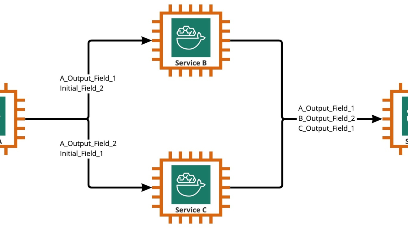
As shown in the following diagram, an ensemble is a collection of two or more models that are orchestrated to run in a linear or nonlinear fashion to produce a single prediction. When stacked linearly, the individual models of an ensemble can be directly invoked for predictions and later consolidated for unification. At times, ensemble models can also be implemented as a serial inference pipeline.

For our use case, the ensemble pipeline is strictly nonlinear, as depicted in the following diagram. Nonlinear ensemble pipelines are theoretically directly acyclic graphs (DAGs). For our use case, this DAG pipeline had both independent models that are run in parallel (Services B, C) and other models that use predictions from previous steps (Service D).

A practice that comes out of the research-driven culture at CCC is the continuous review of technologies that can be leveraged to bring more value to customers. As CCC faced this ensemble challenge, leadership launched a proof-of-concept (POC) initiative to thoroughly assess the offerings from AWS to discover, specifically, whether Amazon SageMaker and other AWS tools could manage the hosting of individual AI models in complex, nonlinear ensembles.

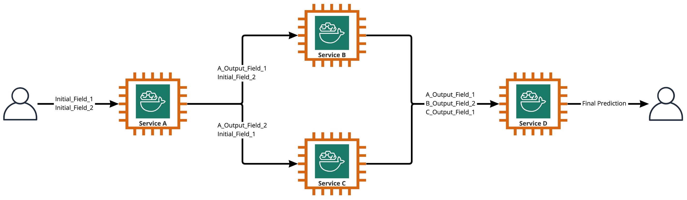
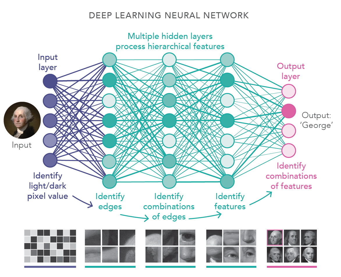
Ensemble explained: In this context, an ensemble is a group of 2 or more AI models that work together to produce 1 overall prediction.

Questions driving the research

Can Amazon SageMaker be used to host complex ensembles of AI models that work together to provide one overall prediction? If so, can SageMaker offer other benefits out of the box, such as increased automation, reliability, monitoring, automatic scaling, and cost-saving measures?

Finding alternative ways to deploy CCC’s AI models using the technological advancements from cloud providers will allow CCC to bring AI solutions to market faster than its competition. Additionally, having more than one deployment architecture provides flexibility when finding the balance between cost and performance based on business priorities.

Based on our requirements, we finalized the following list of features as a checklist for a production-grade deployment architecture:

  • Support for complex ensembles
  • Guaranteed uptime for all components
  • Customizable automatic scaling for deployed AI models
  • Preservation of AI model input and output
  • Usage metrics and logs for all components
  • Cost-saving mechanisms

With a majority of CCC’s AI solutions relying on computer vision models, a new architecture was required to support image and video files that continue to increase in resolution. There was a strong need to design and implement this architecture as an asynchronous model.

After cycles of research and initial benchmarking efforts, CCC determined SageMaker was a perfect fit to meet a majority of their production requirements, especially the guaranteed uptime SageMaker provides for most of its inference components. The default feature of Amazon SageMaker Asynchronous Inference endpoints saving input/output in Amazon S3 simplifies the task of preserving data generated from complex ensembles. Additionally, with each AI model being hosted by its own endpoint, managing automatic scaling policies at the model or endpoint level becomes easier. By simplifying the management, a potential cost-saving benefit from this is development teams can allocate more time towards fine-tuning scaling policies to minimize over-provisioning of compute resources.

Having decided to proceed with using SageMaker as the pivotal component of the architecture, we also realized SageMaker can be part of an even larger architecture, supplemented with many other serverless AWS-managed services. This choice was needed to facilitate the higher-order orchestration and observability needs of this complex architecture.

Firstly, to remove payload size limitations and greatly reduce timeout risk during high-traffic scenarios, CCC implemented an architecture that runs predictions asynchronously using SageMaker Asynchronous Inference endpoints coupled with other AWS-managed services as the core building blocks. Additionally, the user interface for the system follows the fire-and-forget design pattern. In other words, once a user has uploaded their input to the system, nothing more needs to be done. They will be notified when the prediction is available. The figure below illustrates a high-level overview of our asynchronous event-driven architecture. In the upcoming section, let us do a deep dive into the execution flow of the designed architecture.

Step-by-step solution
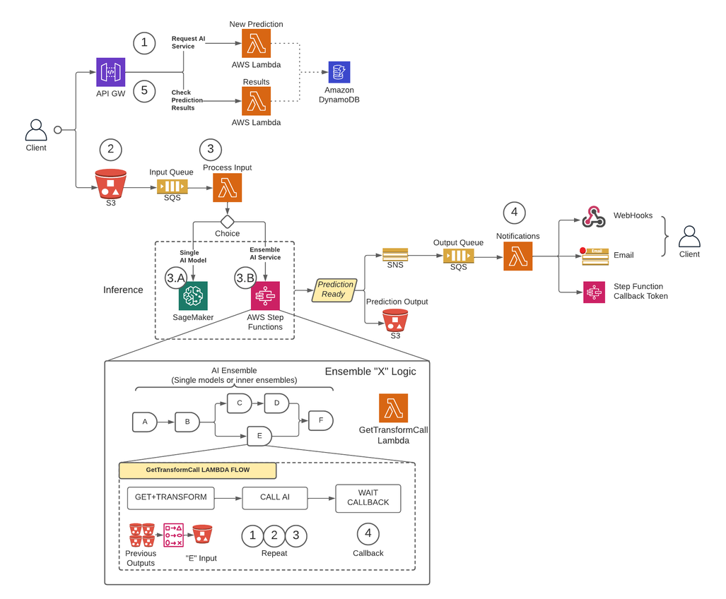
Step 1

A client makes a request to the AWS API Gateway endpoint. The content of the request contains the name of the AI service from which they need a prediction and the desired method of notification.

This request is passed to a Lambda function called New Prediction, whose main tasks are to:

  • Check if the requested service by the client is available.
  • Assign a unique prediction ID to the request. This prediction ID can be used by the user to check the status of the prediction throughout the entire process.
  • Generate an Amazon S3 pre-signed URL that the user will need to use in the next step to upload the input content of the prediction request.
  • Create an entry in Amazon DynamoDB with the information of the received request.

The Lambda function will then return a response through the API Gateway endpoint with a message that includes the prediction ID assigned to the request and the Amazon S3 pre-signed URL.

Step 2

The client securely uploads the prediction input content to an S3 bucket using the pre-signed URL generated in the previous step. Input content depends on the AI service and can be composed of images, tabular data, or a combination of both.

Step 3

The S3 bucket is configured to trigger an event when the user uploads the input content. This notification is sent to an Amazon SQS queue and handled by a Lambda function called Process Input. The Process Input Lambda will obtain the information related to that prediction ID from DynamoDB to get the name of the service to which the request is to be made.

This service can either be a single AI model, in which case the Process Input Lambda will make a request to the SageMaker endpoint that hosts that model (Step 3-A), or it can be an ensemble AI service in which case the Process Input Lambda will make a request to the state machine of the step functions that hosts the ensemble logic (Step 3-B).

In either option (single AI model or ensemble AI service), when the final prediction is ready, it will be stored in the appropriate S3 bucket, and the caller will be notified via the method specified in Step 1 (more details about notifications in Step 4).

Step 3-A

If the prediction ID is associated to a single AI model, the Process Input Lambda will make a request to the SageMaker endpoint that serves the model. In this system, two types of SageMaker endpoints are supported:

  • Asynchronous: The Process Input Lambda makes the request to the SageMaker asynchronous endpoint. The immediate response includes the S3 location where SageMaker will save the prediction output. This request is asynchronous, following the fire-and-forget pattern, and does not block the execution flow of the Lambda function.
  • Synchronous: The Process Input Lambda makes the request to the SageMaker synchronous endpoint. Since it is a synchronous request, Process Input waits for the response, and once obtained, it stores it in S3 in an analogous way that SageMaker asynchronous endpoints would do.

In both cases (synchronous or asynchronous endpoints), the prediction is processed in an equivalent way, storing the output in an S3 bucket. When the asynchronous SageMaker endpoint completes a prediction, an Amazon SNS event is triggered. This behavior is also replicated for synchronous endpoints with additional logic in the Lambda function.

Step 3-B

If the prediction ID is associated with an AI ensemble, the Process Input Lambda will make the request to the step function associated to that AI Ensemble. As mentioned above, an AI Ensemble is an architecture based on a group of AI models working together to generate a single overall prediction. The orchestration of an AI ensemble is done through a step function.

The step function has one step per AI service that comprises the ensemble. Each step will invoke a Lambda function that will prepare its corresponding AI service’s input using different combinations of the output content from previous AI service calls of previous steps. It then makes a call to each AI service which in this context, can wither be a single AI model or another AI ensemble.

The same Lambda function, called GetTransformCall used to handle the intermediate predictions of an AI Ensemble is used throughout the step function, but with different input parameters for each step. This input includes the name of the AI service to be called. It also includes the mapping definition to construct the input for the specified AI service. This is done using a custom syntax that the Lambda can decode, which in summary, is a JSON dictionary where the values should be replaced with the content from the previous AI predictions. The Lambda will download these previous predictions from Amazon S3.

In each step, the GetTransformCall Lambda reads from Amazon S3 the previous outputs that are needed to build the input of the specified AI service. It will then invoke the New Prediction Lambda code previously used in Step 1 and provide the service name, callback method (“step function”), and token needed for the callback in the request payload, which is then saved in DynamoDB as a new prediction record. The Lambda also stores the created input of that stage in an S3 bucket. Depending on whether that stage is a single AI model or an AI ensemble, the Lambda makes a request to a SageMaker endpoint or a different step function that manages an AI ensemble that is a dependency of the parent ensemble.

Once the request is made, the step function enters a pending state until it receives the callback token indicating it can move to the next stage. The action of sending a callback token is performed by a Lambda function called notifications (more details in Step 4) when the intermediate prediction is ready. This process is repeated for each stage defined in the step function until the final prediction is ready.

Step 4

When a prediction is ready and stored in the S3 bucket, an SNS notification is triggered. This event can be triggered in different ways depending on the flow:

  1. Automatically when a SageMaker asynchronous endpoint completes a prediction.
  2. As the very last step of the step function.
  3. By Process Input or GetTransformCall Lambda when a synchronous SageMaker endpoint has returned a prediction.

For B and C, we create an SNS message similar to what A automatically sends.

A Lambda function called notifications is subscribed to this SNS topic. The notifications Lambda will get the information related to the prediction ID from DynamoDB, update the entry with status value to “completed” or “error,” and perform the necessary action depending on the callback mode saved in the database record.

If this prediction is an intermediate prediction of an AI ensemble, as described in step 3-B, the callback mode associated to this prediction will be “step function,” and the database record will have a callback token associated with the specific step in the step function. The notifications Lambda will make a call to the AWS Step Functions API using the method “SendTaskSuccess” or “SendTaskFailure.” This will allow the step function to continue to the next step or exit.

If the prediction is the final output of the step function and the callback mode is “Webhook” [or email, message brokers (Kafka), etc.], then the notifications Lambda will notify the client in the specified way. At any point, the user can request the status of their prediction. The request must include the prediction ID that was assigned in Step 1 and point to the correct URL within API Gateway to route the request to the Lambda function called results.

The results Lambda will make a request to DynamoDB, obtaining the status of the request and returning the information to the user. If the status of the prediction is error, then the relevant details on the failure will be included in the response. If the prediction status is success, an S3 pre-signed URL will be returned for the user to download the prediction content.

Outcomes

Preliminary performance testing results are promising and support the case for CCC to extend the implementation of this new deployment architecture.

Notable observations:

  • Tests reveal strength in processing batch or concurrent requests with high throughput and a 0 percent failure rate during high traffic scenarios.
  • Message queues provide stability within the system during sudden influxes of requests until scaling triggers can provision additional compute resources. When increasing traffic by 3x, average request latency only increased by 5 percent.
  • The price of stability is increased latency due to the communication overhead between the various system components. When user traffic is above the baseline threshold, the added latency can be partially mitigated by providing more compute resources if performance is a higher priority over cost.
  • SageMaker’s asynchronous inference endpoints allow the instance count to be scaled to zero while keeping the endpoint active to receive requests. This functionality enables deployments to continue running without incurring compute costs and scale up from zero when needed in two scenarios: service deployments used in lower test environments and those that have minimal traffic without requiring immediate processing.

Conclusion

As observed during the POC process, the innovative design jointly created by CCC and AWS provides a solid foundation for using Amazon SageMaker with other AWS managed services to host complex multi-modal AI ensembles and orchestrate inference pipelines effectively and seamlessly. By leveraging Amazon SageMaker’s out-of-the-box functionalities like Asynchronous Inference, CCC has more opportunities to focus on specialized business-critical tasks. In the spirit of CCC’s research-driven culture, this novel architecture will continue to evolve as CCC leads the way forward, alongside AWS, in unleashing powerful new AI solutions for clients.­­­

For detailed steps on how to create, invoke, and monitor asynchronous inference endpoints, refer to the documentation, which also contains a sample notebook to help you get started. For pricing information, visit Amazon SageMaker Pricing.

For examples on using asynchronous inference with unstructured data such as computer vision and natural language processing (NLP), refer to Run computer vision inference on large videos with Amazon SageMaker asynchronous endpoints and Improve high-value research with Hugging Face and Amazon SageMaker asynchronous inference endpoints, respectively.


About the Authors

Christopher Diaz is a Lead R&D Engineer at CCC Intelligent Solutions. As a member of the R&D team, he has worked on a variety of projects ranging from ETL tooling, backend web development, collaborating with researchers to train AI models on distributed systems, and facilitating the delivery of new AI services between research and operations teams. His recent focus has been on researching cloud tooling solutions to enhance various aspects of the company’s AI model development lifecycle. In his spare time, he enjoys trying new restaurants in his hometown of Chicago and collecting as many LEGO sets as his home can fit. Christopher earned his Bachelor of Science in Computer Science from Northeastern Illinois University.

Emmy Award winner Sam Kinard is a Senior Manager of Software Engineering at CCC Intelligent Solutions. Based in Austin, Texas, he wrangles the AI Runtime Team, which is responsible for serving CCC’s AI products at high availability and large scale. In his spare time, Sam enjoys being sleep deprived because of his two wonderful children. Sam has a Bachelor of Science in Computer Science and a Bachelor of Science in Mathematics from the University of Texas at Austin.

Jaime Hidalgo is a Senior Systems Engineer at CCC Intelligent Solutions. Before joining the AI research team, he led the company’s global migration to Microservices Architecture, designing, building, and automating the infrastructure in AWS to support the deployment of cloud products and services. Currently, he builds and supports an on-premises data center cluster built for AI training and also designs and builds cloud solutions for the company’s future of AI research and deployment.

Daniel Suarez is a Data Science Engineer at CCC Intelligent Solutions. As a member of the AI Engineering team, he works on the automation and preparation of AI Models in the production, evaluation, and monitoring of metrics and other aspects of ML operations. Daniel received a Master’s in Computer Science from the Illinois Institute of Technology and a Master’s and Bachelor’s in Telecommunication Engineering from Universidad Politecnica de Madrid.

Arunprasath Shankar is a Senior AI/ML Specialist Solutions Architect with AWS, helping global customers scale their AI solutions effectively and efficiently in the cloud. In his spare time, Arun enjoys watching sci-fi movies and listening to classical music.

Justin McWhirter is a Solutions Architect Manager at AWS. He works with a team of amazing Solutions Architects who help customers have a positive experience while adopting the AWS platform. When not at work, Justin enjoys playing video games with his two boys, ice hockey, and off-roading in his Jeep.

Read More

What Is AI Computing?

What Is AI Computing?

The abacus, sextant, slide rule and computer. Mathematical instruments mark the history of human progress.

They’ve enabled trade and helped navigate oceans, and advanced understanding and quality of life.

The latest tool propelling science and industry is AI computing.

AI Computing Defined

AI computing is the math-intensive process of calculating machine learning algorithms, typically using accelerated systems and software. It can extract fresh insights from massive datasets, learning new skills along the way.

It’s the most transformational technology of our time because we live in a data-centric era, and AI computing can find patterns no human could.

For example, American Express uses AI computing to detect fraud in billions of annual credit card transactions. Doctors use it to find tumors, finding tiny anomalies in mountains of medical images.

Three Steps to AI Computing

Before getting into the many use cases for AI computing, let’s explore how it works.

First, users, often data scientists, curate and prepare datasets, a stage called extract/transform/load, or ETL. This work can now be accelerated on NVIDIA GPUs with Apache Spark 3.0, one of the most popular open source engines for mining big data.

Second, data scientists choose or design AI models that best suit their applications.

Some companies design and train their own models from the ground up because they are pioneering a new field or seeking a competitive advantage. This process requires some expertise and potentially an AI supercomputer, capabilities NVIDIA offers.

AI computing and MLops
Machine learning operations (MLOps) describe in finer detail the three major steps of AI computing — ETL (top row), training (lower right) and inference (lower left).

Many companies choose pretrained AI models they can customize as needed for their applications. NVIDIA provides dozens of pretrained models and tools for customizing them on NGC, a portal for software, services, and support.

Third, companies sift their data through their models. This key step, called inference, is where AI delivers actionable insights.

The three-step process involves hard work, but there’s help available, so everyone can use AI computing.

For example, NVIDIA TAO Toolkit can collapse the three steps into one using transfer learning, a way of tailoring an existing AI model for a new application without needing a large dataset. In addition, NVIDIA LaunchPad gives users hands-on training in deploying models for a wide variety of use cases.

Inside an AI Model

AI models are called neural networks because they’re inspired by the web-like connections in the human brain.

If you slice into one of these AI models, it might look like a mathematical lasagna, made up of layers of linear algebra equations. One of the most popular forms of AI is called deep learning because it uses many layers.

An example of a deep learning model used in AI computing
An example of a deep learning model that identifies an image. From an article on deep learning for the U.S. National Academy of Sciences. Image credit: Lucy Reading-Ikkanda (artist).

If you zoom in, you’d see each layer is made up of stacks of equations. Each represents the likelihood that one piece of data is related to another.

AI computing multiplies together every stack of equations in every layer to find patterns. It’s a huge job that requires highly parallel processors sharing massive amounts of data on fast computer networks.

GPU Computing Meets AI

GPUs are the de facto engines of AI computing.

NVIDIA debuted the first GPU in 1999 to render 3D images for video games, a job that required massively parallel calculations.

GPU computing soon spread to use in graphics servers for blockbuster movies. Scientists and researchers packed GPUs into the world’s largest supercomputers to study everything from the chemistry of tiny molecules to the astrophysics of distant galaxies.

When AI computing emerged more than a decade ago, researchers were quick to embrace NVIDIA’s programmable platform for parallel processing. The video below celebrates this brief history of the GPU.

The History of AI Computing

The idea of artificial intelligence goes back at least as far as Alan Turing, the British mathematician who helped crack coded messages during WWII.

“What we want is a machine that can learn from experience,” Turing said in a 1947 lecture in London.

AI visionary Alan Turing
Alan Turing

Acknowledging his insights, NVIDIA named one of its computing architectures for him.

Turing’s vision became a reality in 2012 when researchers developed AI models that could recognize images faster and more accurately than humans could. Results from the ImageNet competition also greatly accelerated progress in computer vision.

Today, companies such as Landing AI, founded by machine learning luminary Andrew Ng, are applying AI and computer vision to make manufacturing more efficient. And AI is bringing human-like vision to sports, smart cities and more.

AI Computing Starts Up Conversational AI

AI computing made huge inroads in natural language processing after the invention of the transformer model in 2017. It debuted a machine-learning technique called “attention” that can capture context in sequential data like text and speech.

Today, conversational AI is widespread. It parses sentences users type into search boxes. It reads text messages when you’re driving, and lets you dictate responses.

These large language models are also finding applications in drug discovery, translation, chatbots, software development, call center automation and more.

AI + Graphics Create 3D Worlds

Users in many, often unexpected, areas are feeling the power of AI computing.

The latest video games achieve new levels of realism thanks to real-time ray tracing and NVIDIA DLSS, which uses AI to deliver ultra-smooth game play on the GeForce RTX platform.

That’s just the start. The emerging field of neural graphics will speed the creation of virtual worlds to populate the metaverse, the 3D evolution of the internet.

Neural graphics combine AI computing and graphics
Neural graphics accelerate design and development of virtual worlds to populate the metaverse, the 3D internet.

To kickstart that work, NVIDIA released several neural graphics tools in August.

Use Cases for AI Computing

Cars, Factories and Warehouses

Car makers are embracing AI computing to deliver a smoother, safer driving experience and deliver smart infotainment capabilities for passengers.

Mercedes-Benz is working with NVIDIA to develop software-defined vehicles. Its upcoming fleets will deliver intelligent and automated driving capabilities powered by an NVIDIA DRIVE Orin centralized computer. The systems will be tested and validated in the data center using DRIVE Sim software, built on NVIDIA Omniverse, to ensure they can safely handle all types of scenarios.

At CES, the automaker announced it will also use Omniverse to design and plan manufacturing and assembly facilities at its sites worldwide.

BMW Group is also among many companies creating AI-enabled digital twins of factories in NVIDIA Omniverse, making plants more efficient. It’s an approach also adopted by consumer giants such as PepsiCo for its logistic centers as shown in the video below.

Inside factories and warehouses, autonomous robots further enhance efficiency in manufacturing and logistics. Many are powered by the NVIDIA Jetson edge AI platform and trained with AI in simulations and digital twins using NVIDIA Isaac Sim.

In 2022, even tractors and lawn mowers became autonomous with AI.

In December, Monarch Tractor, a startup based in Livermore, Calif., released an AI-powered electric vehicle to bring automation to agriculture. In May, Scythe, based in Boulder, Colo., debuted its M.52 (below), an autonomous electric lawn mower packing eight cameras and more than a dozen sensors.

Securing Networks, Sequencing Genes

The number and variety of use cases for AI computing are staggering.

Cybersecurity software detects phishing and other network threats faster with AI-based techniques like digital fingerprinting.

In healthcare, researchers broke a record in January 2022 sequencing a whole genome in well under eight hours thanks to AI computing. Their work (described in the video below) could lead to cures for rare genetic diseases.

AI computing is at work in banks, retail shops and post offices. It’s used in telecom, transport and energy networks, too.

For example, the video below shows how Siemens Gamesa is using AI models to simulate wind farms and boost energy production.

As today’s AI computing techniques find new applications, researchers are inventing newer and more powerful methods.

Another powerful class of neural networks, diffusion models, became popular in 2022 because they could turn text descriptions into fascinating images. Researchers expect these models will be applied to many uses, further expanding the horizon for AI computing.

Read More

Fully Autonomous Real-World Reinforcement Learning with Applications to Mobile Manipulation

Fully Autonomous Real-World Reinforcement Learning with Applications to Mobile Manipulation

Reinforcement learning provides a conceptual framework for autonomous agents to learn from experience, analogously to how one might train a pet with treats. But practical applications of reinforcement learning are often far from natural: instead of using RL to learn through trial and error by actually attempting the desired task, typical RL applications use a separate (usually simulated) training phase. For example, AlphaGo did not learn to play Go by competing against thousands of humans, but rather by playing against itself in simulation. While this kind of simulated training is appealing for games where the rules are perfectly known, applying this to real world domains such as robotics can require a range of complex approaches, such as the use of simulated data, or instrumenting real-world environments in various ways to make training feasible under laboratory conditions. Can we instead devise reinforcement learning systems for robots that allow them to learn directly “on-the-job”, while performing the task that they are required to do? In this blog post, we will discuss ReLMM, a system that we developed that learns to clean up a room directly with a real robot via continual learning.


We evaluate our method on different tasks that range in difficulty. The top-left task has uniform white blobs to pickup with no obstacles, while other rooms have objects of diverse shapes and colors, obstacles that increase navigation difficulty and obscure the objects and patterned rugs that make it difficult to see the objects against the ground.

AI’s Leg Up: Startup Accelerates Robotics Simulation for $8 Trillion Food Market

AI’s Leg Up: Startup Accelerates Robotics Simulation for $8 Trillion Food Market

Robots are finally getting a grip.

Developers have been striving to close the gap on robotic gripping for the past several years, pursuing applications for multibillion-dollar industries. Securely gripping and transferring fast-moving items on conveyor belts holds vast promise for businesses.

Soft Robotics, a Bedford, Mass., startup, is harnessing NVIDIA Isaac Sim to help close the sim to real gap for a handful of robotic gripping applications. One area is perfecting gripping for pick and placement of foods for packaging.

Food packaging and processing companies are using the startup’s mGripAI system, which combines soft grasping with 3D vision and AI to grasp delicate foods such as proteins, produce and bakery items without damage.

“We’re selling the hands, the eyes and the brains of the picking solution,” said David Weatherwax, senior director of software engineering at Soft Robotics.

Unlike other industries that have adopted robotics, the $8 trillion food market has been slow to develop robots to handle variable items in unstructured environments, says Soft Robotics.

The company, founded in 2013, recently landed $26 million in Series C funding from Tyson Ventures, Marel and Johnsonville Ventures.

Companies such as Tyson Foods and Johnsonville are betting on adoption of robotic automation to help improve safety and increase production in their facilities. Both companies rely on Soft Robotics technologies.

Soft Robotics is a member of the NVIDIA Inception program, which provides companies with GPU support and AI platforms guidance.

Getting a Grip With Synthetic Data

Soft Robotics develops unique models for every one of its gripping applications, each requiring specific datasets. And picking from piles of wet, slippery chicken and other foods can be a tricky challenge.

We’re all in on Omniverse and Isaac Sim, and that’s been working great for us, said  Weatherwax.

Utilizing Omniverse and Isaac Sim, the company can create 3D renderings of chicken parts with different backgrounds, like on conveyor belts or in bins, and with different lighting scenarios.

The company taps into Isaac Replicator to develop synthetic data, generating hundreds of thousands of images per model and distributing that among an array of instances in the cloud. Isaac Replicator is a set of tools, APIs and workflows for generating synthetic data using Isaac Sim.

It also runs pose estimation models to help its gripping system see the angle of the item to pick.

NVIDIA A100 Tensor Core GPUs on site enable Soft Robotics to run split-second inference with the unique models for each application in these food-processing facilities. Meanwhile, simulation and training in Isaac Sim offers access to NVIDIA A100 GPUs for scaling up workloads.

“Our current setup is fully synthetic, which allows us to rapidly deploy new applications,” said Weatherwax. “We’re all in on Omniverse and Isaac Sim, and that’s been working great for us.”

Solving Issues With Occlusion, Lighting 

A big challenge at Soft Robotics is solving issues with occlusion for an understanding of how different pieces of chicken stack up and overlap one another when dumped into a pile. “How those form can be pretty complex,” he said.

A key thing for us is the lighting, so the NVIDIA RTX-driven ray tracing is really important, said Weatherwax.

Glares on wet chicken can potentially throw off detection models. “A key thing for us is the lighting, so the NVIDIA RTX-driven ray tracing is really important,” he added.

But where it really gets interesting is modeling it all in 3D and figuring out in a split second which item is the least obstructed in a pile and most accessible for a robot gripper to pick and place.

Building synthetic data sets with physics-based accuracy, Omniverse enables Soft Robotics to create such environments. “One of the big challenges we have is how all these amorphous objects form into a pile.”

Boosting Production Line Pick Accuracy

Production lines in food processing plants can move fast. But robots deployed with application-specific models promise to handle as many as 100 picks per minute.

Still a work in progress, success in such tasks hinges on accurate representations of piles of items, supported by training datasets that consider every possible way items can fall into a pile.

The objective is to provide the robot with the best available pick from a complex and dynamic environment. If food items fall off the conveyor belt or otherwise become damaged, then it is considered waste, which directly impacts yield.

Driving Production Gains 

Meat-packing companies rely on lines of people for processing chicken, but like so many other industries they have faced employee shortages. Some that are building new plants for food processing can’t even attract enough workers at launch, said Weatherwax.

“They are having a lot of staffing challenges, so there’s a push to automate,” he said.

The Omniverse-driven work for food processing companies has delivered a more than 10x increase in its simulation capacity, accelerating deployments times for AI picking systems from months to days.

And that’s enabling Soft Robotics customers to get a grip on more than just deploying automated chicken-picking lines — it’s ensuring that they’re covered for an employment challenge that has hit many industries, especially those with increased injury and health risks.

“Handling raw chicken is a job better suited for a robot,” he said.

Download Isaac Sim here to use the  Replicator features.

Read More