Monthly Archives: March 2023

Language models are statistical methods predicting the succession of tokens in sequences, using natural text. Large language models (LLMs) are neural network-based language models with hundreds of millions (BERT) to over a trillion parameters (MiCS), and whose size makes single-GPU training impractical. LLMs’ generative abilities make them popular for text synthesis, summarization, machine translation, and more.

The size of an LLM and its training data is a double-edged sword: it brings modeling quality, but entails infrastructure challenges. The model itself is often too big to fit in memory of a single GPU device or on the multiple devices of a multi-GPU instance. These factors require training an LLM over large clusters of accelerated machine learning (ML) instances. In the past few years, numerous customers have been using the AWS Cloud for LLM training.

In this post, we dive into tips and best practices for successful LLM training on Amazon SageMaker Training. SageMaker Training is a managed batch ML compute service that reduces the time and cost to train and tune models at scale without the need to manage infrastructure. Within one launch command, Amazon SageMaker launches a fully functional, ephemeral compute cluster running the task of your choice, and with enhanced ML features such as metastore, managed I/O, and distribution. The post covers all the phases of an LLM training workload and describes associated infrastructure features and best practices. Some of the best practices in this post refer specifically to ml.p4d.24xlarge instances, but most are applicable to any instance type. These best practices allow you to train LLMs on SageMaker in the scale of dozens to hundreds of millions of parameters.

Regarding the scope of this post, note the following:

• We don’t cover neural network scientific design and associated optimizations. Amazon.Science features numerous scientific publications, including and not limited to LLMs.
• Although this post focuses on LLMs, most of its best practices are relevant for any kind of large-model training, including computer vision and multi-modal models, such as Stable Diffusion.

Best practices

We discuss the following best practices in this post:

• Compute – SageMaker Training is a great API to launch CPU dataset preparation jobs and thousand-scale GPU jobs.
• Storage – We see data loading and checkpointing done in two ways, depending on skills and preferences: with an Amazon FSx Lustre file system, or Amazon Simple Storage Service (Amazon S3) only.
• Parallelism – Your choice of distributed training library is crucial for appropriate use of the GPUs. We recommend using a cloud-optimized library, such as SageMaker sharded data parallelism, but self-managed and open-source libraries can also work.
• Networking – Make sure EFA and NVIDIA GPUDirectRDMA are enabled, for fast inter-machine communication.
• Resiliency – At scale, hardware failures can happen. We recommend checkpointing regularly. Every few hours is common.

Region selection

Instance type and desired capacity is a determining factor for Region selection. For the Regions supported by SageMaker and the Amazon Elastic Compute Cloud (Amazon EC2) instance types that are available in each Region, see Amazon SageMaker Pricing. In this post, we assume the training instance type to be a SageMaker-managed ml.p4d.24xlarge.

We recommend working with your AWS account team or contacting AWS Sales to determine the appropriate Region for your LLM workload.

Data preparation

LLM developers train their models on large datasets of naturally occurring text. Popular examples of such data sources include Common Crawl and The Pile. Naturally occurring text may contain biases, inaccuracies, grammatical errors, and syntax variations. An LLM’s eventual quality significantly depends on the selection and curation of the training data. LLM training data preparation is an active area of research and innovation in the LLM industry. The preparation of a natural language processing (NLP) dataset abounds with share-nothing parallelism opportunities. In other words, there are steps that can be applied to units of works—source files, paragraphs, sentences, words—without requiring inter-worker synchronization.

The SageMaker jobs APIs, namely SageMaker Training and SageMaker Processing, excel for this type of tasks. They enable developers to run an arbitrary Docker container over a fleet of multiple machines. In the case of the SageMaker Training API, the computing fleet can be heterogeneous. Numerous distributed computing frameworks have been used on SageMaker, including Dask, Ray, and also PySpark, which have a dedicated AWS-managed container and SDK in SageMaker Processing.

When you launch a job with multiple machines, SageMaker Training and Processing run your code one time per machine. You don’t need to use a particular distributed computing framework to write a distributed application: you can write the code of your choice, which will run one time per machine, to realize share-nothing parallelism. You can also write or install the inter-node communication logic of your choice.

Data loading

There are multiple ways to store the training data and move it from its storage to the accelerated compute nodes. In this section, we discuss the options and best practices for data loading.

SageMaker storage and loading options

A typical LLM dataset size is in the hundreds of millions of text tokens, representing a few hundred gigabytes. SageMaker-managed clusters of ml.p4d.24xlarge instances propose several options for dataset storage and loading:

• On-node NVMe SSD – ml.P4d.24xlarge instances are equipped with 8TB NVMe, available under /opt/ml/input/data/<channel> if you use SageMaker File mode, and at /tmp. If you’re seeking the simplicity and performance of a local read, you can copy your data to the NVMe SSD. The copy can either be done by SageMaker File mode, or by your own code, for example using multi-processed Boto3 or S5cmd.
• FSx for Lustre – On-node NVMe SSDs are limited in size, and require ingestion from Amazon S3 at each job or warm cluster creation. If you’re looking to scale to larger datasets while maintaining low-latency random access, you can use FSx for Lustre. Amazon FSx is an open-source parallel file system, popular in high-performance computing (HPC). FSx for Lustre uses distributed file storage (stripping) and physically separates file metadata from file content to achieve high-performance read/writes.
• SageMaker FastFile Mode – FastFile Mode (FFM) is a SageMaker-only feature that presents remote S3 objects in SageMaker-managed compute instances under a POSIX-compliant interface, and streams them only upon reading, using FUSE. FFM reads results in S3 calls that stream remote files block by block. As a best practice to avoid errors related to Amazon S3 traffic, FFM developers should aim to keep the underlying number of S3 calls reasonable, for example by reading files sequentially and with a controlled amount of parallelism.
• Self-managed data loading – Of course, you may also decide to implement your own, fully custom data loading logic, using proprietary or open-source code. Some reasons to use self-managed data loading are to facilitate a migration by reusing already-developed code, to implement custom error handling logic, or to have more control on underlying performance and sharding. Examples of libraries you may use for self-managed data loading include torchdata.datapipes (previously AWS PyTorch S3 Plugin) and Webdataset. The AWS Python SDK Boto3 may also be combined with Torch Dataset classes to create custom data loading code. Custom data loading classes also enable the creative use of SageMaker Training heterogeneous clusters, to finely adapt the CPU and GPU balance to a given workload.

For more information about those options and how to choose them, refer to Choose the best data source for your Amazon SageMaker training job.

Best practices for large-scale interaction with Amazon S3

Amazon S3 is capable of handling LLM workloads, both for data reading and checkpointing. It supports a request rate of 3,500 PUT/COPY/POST/DELETE or 5,500 GET/HEAD requests per second per prefix in a bucket. However, this rate is not necessarily available by default. Instead, as the request rate for a prefix grows, Amazon S3 automatically scales to handle the increased rate. For more information, refer to Why am I getting 503 Slow Down errors from Amazon S3 when the requests are within the supported request rate per prefix.

If you expect high-frequency Amazon S3 interaction, we recommend the following best practices:

• Try to read and write from multiple S3 buckets and prefixes. For example, you can partition training data and checkpoints across different prefixes.
• Check Amazon S3 metrics in Amazon CloudWatch to track request rates.
• Try to minimize the amount of simultaneous PUT/GET:
  • Have fewer processes using Amazon S3 at the same time. For example, if eight processes per nodes need to checkpoint to Amazon S3, you can reduce PUT traffic by a factor of 8 by checkpointing hierarchically: first within-node, then from the node to Amazon S3.
  • Read multiple training records from a single file or S3 GET, instead of using an S3 GET for every training record.
  • If you use Amazon S3 via SageMaker FFM, SageMaker FFM makes S3 calls to fetch files chunk by chunk. To limit the Amazon S3 traffic generated by FFM, we encourage you to read files sequentially and limit the number files opened in parallel.

If you have a Developer, Business, or Enterprise Support plan, you can open a technical support case about S3 503 Slow Down errors. But first make sure you have followed the best practices, and get the request IDs for the failed requests.

Training parallelism

LLMs commonly have dozens to hundreds of billions of parameters, making them too big to fit within a single NVIDIA GPU card. LLM practitioners have developed several open-source libraries facilitating the distributed computation of LLM training, including FSDP, DeepSpeed and Megatron. You can run those libraries in SageMaker Training, but you can also use SageMaker distributed training libraries, which have been optimized for the AWS Cloud and provide a simpler developer experience. Developers have two choices for distributed training of their LLM on SageMaker: distributed libraries or self-managed.

SageMaker distributed libraries

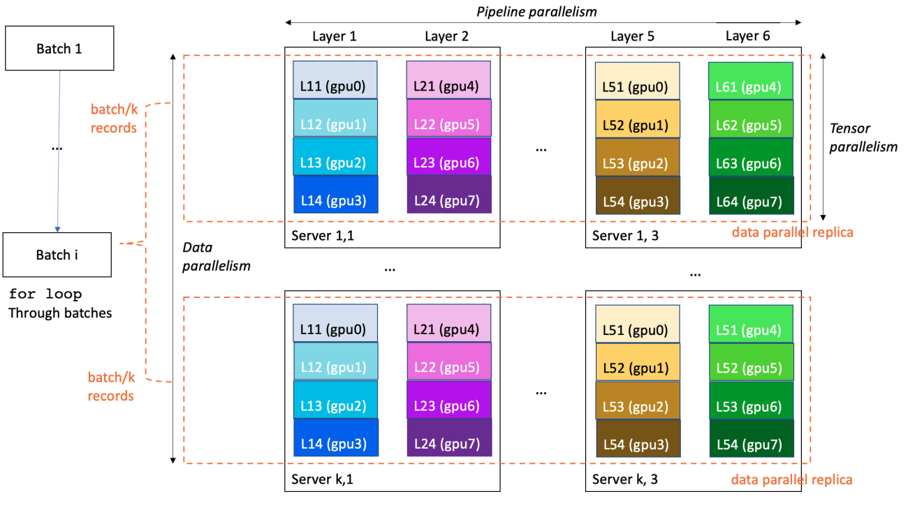
To provide you with improved distributed training performance and usability, SageMaker Training proposes several proprietary extensions to scale TensorFlow and PyTorch training code. LLM training is often conducted in a 3D-parallelism fashion:

• Data parallelism splits and feeds the training mini-batches to multiple identical replicas of the model, to increase processing speed
• Pipeline parallelism attributes various layers of the model to different GPUs or even instances, in order to scale model size beyond a single GPU and a single server
• Tensor parallelism splits a single layer into multiple GPUs, usually within the same server, to scale individual layers to sizes exceeding a single GPU

In the following example, a 6-layer model is trained on a cluster of k*3 servers with 8*k*3 GPUs (8 GPUs per server). Data parallelism degree is k, pipeline parallelism 6, and tensor parallelism 4. Each GPU in the cluster contains one-fourth of a model layer, and a full model is partitioned over three servers (24 GPUs in total).

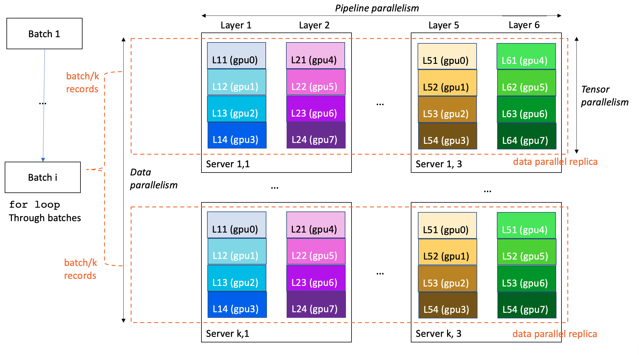
The following are specifically relevant for LLMs:

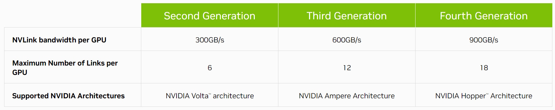
• SageMaker distributed model parallel – This library uses graph partitioning to produce intelligent model partitioning optimized for speed or memory. SageMaker distributed model parallel exposes the latest and greatest large-model training optimization, including data parallelism, pipeline parallelism, tensor parallelism, optimizer state sharding, activation checkpointing, and offloading. With the SageMaker distributed model parallel library, we documented a 175-billion parameter model training over 920 NVIDIA A100 GPUs. For more information, refer to Train 175+ billion parameter NLP models with model parallel additions and Hugging Face on Amazon SageMaker.
• SageMaker sharded data parallel – In MiCS: Near-linear Scaling for Training Gigantic Model on Public Cloud, Zhang et al. introduce a low-communication model parallel strategy that partitions models over a data parallel group only, instead of the whole cluster. With MiCS, AWS scientists were able to achieve 176 teraflops per GPU (56.4% of the theoretical peak) for training a 210-layer 1.06-trillion-parameter model on EC2 P4de instances. MiCS is now available for SageMaker Training customers as SageMaker sharded data parallel.

SageMaker distributed training libraries provide high performance and a simpler developer experience. In particular, developers don’t need to write and maintain a custom parallel process launcher or use a framework-specific launch tool, because the parallel launcher is built into the job launch SDK.

Self-managed

With SageMaker Training, you have the freedom to use the framework and scientific paradigm of your choice. In particular, if you want to manage distributed training yourself, you have two options to write your custom code:

• Use an AWS Deep Learning Container (DLC) – AWS develops and maintains DLCs, providing AWS-optimized Docker-based environments for top open-source ML frameworks. SageMaker Training has a unique integration allowing to you pull and run AWS DLCs with external, user-defined entry point. For LLM training in particular, AWS DLCs for TensorFlow, PyTorch, Hugging Face, and MXNet are particularly relevant. Using a framework DLC allows you to use framework-native parallelism, such as PyTorch Distributed, without having to develop and manage your own Docker images. Additionally, our DLCs feature an MPI integration, which allows you to launch parallel code easily.
• Write a custom SageMaker-compatible Docker image – You can bring your own (BYO) image (see Use Your Own Training Algorithms and Amazon SageMaker Custom Training containers), either starting from scratch or extending an existing DLC image. When using a custom image for LLM training on SageMaker, it’s particularly important to verify the following:
  • Your image contains EFA with appropriate settings (discussed more later in this post)
  • Your image contains an NVIDIA NCCL communication library, enabled with GPUDirectRDMA

Customers have been able to use a number of self-managed distributed training libraries, including DeepSpeed.

Communications

Given the distributed nature of an LLM training job, inter-machine communication is critical to the feasibility, performance, and costs of the workload. In this section, we present key features for inter-machine communication and conclude with tips for installation and tuning.

Elastic Fabric Adapter

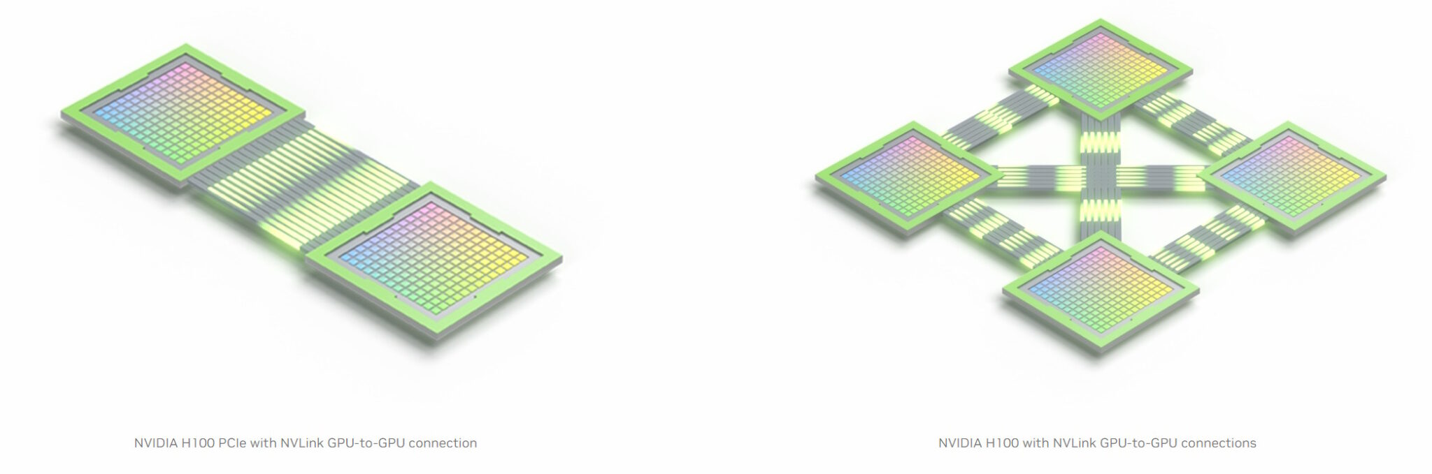
In order to accelerate ML applications, and improve performances by achieving flexibility, scalability, and elasticity provided by the cloud, you can take advantage of Elastic Fabric Adapter (EFA) with SageMaker. In our experience, using EFA is a requirement to get satisfactory multi-node LLM training performance.

An EFA device is a network interface attached to EC2 instances managed by SageMaker during the run of the training jobs. EFA is available on specific families of instances, including the P4d. EFA networks are capable of achieving several hundreds of Gbps of throughput.

Associated to EFA, AWS has introduced the Scalable Reliable Datagram (SRD), an ethernet-based transport inspired by the InfiniBand Reliable Datagram, evolved with relaxed packet ordering constraint. For more information about EFA and SRD, refer to In the search for performance, there’s more than one way to build a network, the video How EFA works and why we don’t use infiniband in the cloud, and the research paper A Cloud-Optimized Transport Protocol for Elastic and Scalable HPC from Shalev et al.

You can add EFA integration on compatible instances to SageMaker existing Docker containers, or custom containers that can be used for training ML models using SageMaker jobs. For more information, refer to Run Training with EFA. EFA is exposed via the open-source Libfabric communication package. However, LLM developers rarely directly program it with Libfabric, and usually instead rely on the NVIDIA Collective Communications Library (NCCL).

AWS-OFI-NCCL plugin

In distributed ML, EFA is most often used with the NVIDIA Collective Communications Library (NCCL). NCCL is an NVIDIA-developed open-source library implementing inter-GPU communication algorithms. Inter-GPU communication is a cornerstone of LLM training that catalyzes scalability and performance. It is so critical to DL training that the NCCL is often directly integrated as a communication backend in deep learning training libraries, so that LLM developers use it—sometimes without noticing—from their preferred Python DL development framework. To use the NCCL on EFA, LLM developers use the AWS-developed AWS OFI NCCL plugin, which maps NCCL calls to the Libfabric interface used by EFA. We recommend using the latest version of AWS OFI NCCL to benefit from recent improvements.

To verify that the NCCL uses EFA, you should set the environment variable NCCL_DEBUG to INFO, and check in the logs that EFA is loaded by the NCCL:

...
NCCL INFO NET/OFI Selected Provider is efa
NCCL INFO Using network AWS Libfabric
...

For more information about the NCCL and EFA configuration, refer to Test your EFA and NCCL configuration. You can further customize the NCCL with several environment variables. Note that effective in NCCL 2.12 and above, AWS contributed an automated communication algorithm selection logic for EFA networks (NCCL_ALGO can be left unset).

NVIDIA GPUDirect RDMA over EFA

With the P4d instance type, we introduced GPUDirect RDMA (GDR) over EFA fabric. It enables network interface cards (NICs) to directly access GPU memory, making remote GPU-to-GPU communication across NVIDIA GPU-based EC2 instances faster, reducing orchestration overhead on CPUs and user applications. GDR is used under the hood by the NCCL, when feasible.

GDR usage appears in inter-GPU communication when the log level is set to INFO, as in the following code:

NCCL INFO Channel 00 : 9[101d0] -> 0[101c0] [receive] via NET/AWS Libfabric/1/GDRDMA
NCCL INFO Channel 00 : 1[101d0] -> 8[101c0] [send] via NET/AWS Libfabric/1/GDRDMA

Using EFA in AWS Deep Learning Containers

AWS maintains Deep Learning Containers (DLCs), many of which come with AWS-managed Dockerfiles and built containing EFA, AWS OFI NCCL, and NCCL. The following GitHub repos offer examples with PyTorch and TensorFlow. You don’t need to install those libraries yourself.

Using EFA in your own SageMaker Training container

If you create your own SageMaker Training container and want to use the NCCL over EFA for accelerated inter-node communication, you need to install EFA, NCCL, and AWS OFI NCCL. For more information, refer to Run Training with EFA. Additionally, you should set the following environment variables in your container or in your entry point code:

• FI_PROVIDER="efa" specifies the fabric interface provider
• NCCL_PROTO=simple instructs the NCCL to use a simple protocol for communication (currently, the EFA provider doesn’t support LL protocols; enabling them could lead to data corruption)
• FI_EFA_USE_DEVICE_RDMA=1 uses the device’s RDMA functionality for one-sided and two-sided transfer
• NCCL_LAUNCH_MODE="PARALLEL"
• NCCL_NET_SHARED_COMMS="0"

Orchestration

Managing the lifecycle and workload of dozens to hundreds of compute instances requires orchestration software. In this section, we offer best practices for LLM orchestration

Within-job orchestration

Developers must write both server-side training code and client-side launcher code in most distributed frameworks. Training code runs on training machines, whereas client-side launcher code launches the distributed workload from a client machine. There is little standardization today, for example:

• In PyTorch, developers can launch multi-machine tasks using torchrun, torchx, torch.distributed.launch (deprecation path), or torch.multiprocessing.spawn
• DeepSpeed proposes its own deepspeed CLI launcher and also supports MPI launch
• MPI is a popular parallel computing framework that has the benefit of being ML-agnostic and reasonably tenured, and therefore stable and documented, and is increasingly seen in distributed ML workloads

In a SageMaker Training cluster, the training container is launched one time on each machine. Consequently, you have three options:

• Native launcher – You can use as an entry point the native launcher of a particular DL framework, for example a torchrun call, which will itself spawn multiple local process and establish communications across instances.
• SageMaker MPI integration – You can use SageMaker MPI integration, available in our AWS DLC, or self-installable via sagemaker-training-toolkit, to directly run your entry point code N times per machine. This has the benefit of avoiding the use of intermediary, framework-specific launcher scripts in your own code.
• SageMaker distributed libraries – If you use the SageMaker distributed libraries, you can focus on the training code and don’t have to write launcher code at all! SageMaker distributed launcher code is built into the SageMaker SDK.

Inter-job orchestration

LLM projects often consist of multiple jobs: parameter search, scaling experiments, recovery from errors, and more. In order to start, stop, and parallelize training tasks, it’s important to use a job orchestrator. SageMaker Training is a serverless ML job orchestrator that provisions transient compute instances immediately upon request. You pay only for what you use, and clusters get decommissioned as soon as your code ends. With SageMaker Training Warm Pools, you have the option to define a time-to-live on training clusters, in order to reuse the same infrastructure across jobs. This reduces iteration time and inter-job placement variability. SageMaker jobs can be launched from a variety of programming languages, including Python and CLI.

There is a SageMaker-specific Python SDK called the SageMaker Python SDK and implemented via the sagemaker Python library, but its use is optional.

Increasing quotas for training jobs with a large and long training cluster

SageMaker has default quotas on resources, designed to prevent unintentional usage and costs. To train an LLM using a big cluster of high-end instances running for a long time, you’ll likely need to increase the quotas in the following table.

See AWS service quotas how to view your quota values and request a quota increase. On-Demand, Spot Instance, and training warm pools quotas are tracked and modified separately.

If you decide to keep the SageMaker Profiler activated, be aware that every training job launches a SageMaker Processing job, each consuming one ml.m5.2xlarge instance. Confirm that your SageMaker Processing quotas are high enough to accommodate the expected training job concurrency. For example, if you want to launch 50 Profiler-enabled training jobs running concurrently, you’ll need to raise the ml.m5.2xlarge for processing job usage limit to 50.

Additionally, to launch a long-running job, you’ll need to explicitly set the Estimator max_run parameter to the desired maximum duration for the training job in seconds, up to the quota value of the longest runtime for a training job.

Monitoring and resiliency

Hardware failure is extremely rare at the scale of a single instance and becomes more and more frequent as the number of instances used simultaneously increases. At typical LLM scale—hundreds to thousands of GPUs used 24/7 for weeks to months—hardware failures are near-certain to happen. Therefore, an LLM workload must implement appropriate monitoring and resiliency mechanisms. Firstly, it’s important to closely monitor LLM infrastructure, to limit the impact of failures and optimize the use of compute resources. SageMaker Training proposes several features for this purpose:

• Logs are automatically sent to CloudWatch Logs. Logs include your training script stdout and stderr. In MPI-based distributed training, all MPI workers send their logs to the leader process.
• System resource utilization metrics like memory, CPU usage, and GPU usage, are automatically sent to CloudWatch.
• You can define custom training metrics that will be sent to CloudWatch. The metrics are captured from logs based on regular expressions you set. Third-party experiment packages like the AWS Partner offering Weights & Biases can be used with SageMaker Training (for an example, see Optimizing CIFAR-10 Hyperparameters with W&B and SageMaker).
• SageMaker Profiler allows you to inspect infrastructure usage and get optimization recommendations.
• Amazon EventBridge and AWS Lambda allow you to create automated client logic reacting to events such as job failures, successes, S3 file uploads, and more.
• SageMaker SSH Helper is a community-maintained open-source library allowing to you connect to training job hosts through SSH. It can be helpful to inspect and troubleshoot code runs on specific nodes.

In addition to monitoring, SageMaker also brings equipment for job resiliency:

• Cluster health checks – Before your job starts, SageMaker runs GPU health checks and verifies NCCL communication on GPU instances, replacing any faulty instances if necessary in order to ensure your training script starts running on a healthy cluster of instances. Health checks are currently enabled for P and G GPU-based instance types.
• Built-in retries and cluster update – You can configure SageMaker to automatically retry training jobs that fails with a SageMaker internal server error (ISE). As part of retrying a job, SageMaker will replace any instances that encountered unrecoverable GPU errors with fresh instances, reboot all healthy instances, and start the job again. This results in faster restarts and workload completion. Cluster update is currently enabled for P and G GPU-based instance types. You can add in your own applicative retry mechanism around the client code that submits the job, to handle other types of launch errors, such as like exceeding your account quota.
• Automated checkpoint to Amazon S3 – This helps you checkpoint your progress and reload a past state on new jobs.

To benefit from node-level replacement, your code must error. Collectives may hang, instead of erroring, when a node fails. Therefore, to have prompt remediation, properly set a timeout on your collectives and have the code throw an error when it is reached.

Some customers set up a monitoring client to monitor and act in case of job hangs or applicative convergence stopping, by monitoring CloudWatch logs and metrics for abnormal patterns like no logs written or 0% GPU usage to hint for a hang, convergence stopping, and auto stop/retry the job.

Deep dive on checkpointing

The SageMaker checkpoint feature copies everything you write on /opt/ml/checkpoints back to Amazon S3 as the URI specified in the checkpoint_s3_uri SDK parameter. When a job starts or restarts, everything written at that URI is sent back to all the machines, at /opt/ml/checkpoints. This is convenient if you want all nodes to have access to all checkpoints, but at scale—when you have many machines or many historical checkpoints, it can lead to long download times and too high traffic on Amazon S3. Additionally, in tensor and pipeline parallelism, the workers need only a fraction of the checkpointed model, not all of it. If you face those limitations, we recommend the following options:

• Checkpointing to FSx for Lustre – Thanks to high-performance random I/O, you can define the sharding and file attribution scheme of your choice
• Self-managed Amazon S3 checkpointing – For examples of Python functions that can be used to save and read checkpoints in a non-blocking fashion, refer to Saving Checkpoints

We strongly suggest checkpointing your model every few hours, for example 1–3 hours, depending on associated overhead and costs.

Front end and user management

User management is a key usability strength of SageMaker compared to legacy shared HPC infrastructure. SageMaker Training permissions are ruled by several AWS Identity and Access Management (IAM) abstractions:

• Principals—users and systems—are given permission to launch resources
• Training jobs carry roles themselves, which allow them to have permissions of their own, for example regarding data access and service invocation

Additionally, in 2022 we added SageMaker Role Manager to facilitate the creation of persona-driven permissions.

Conclusion

With SageMaker Training, you can reduce costs and increase iteration speed on your large-model training workload. We have documented success stories in numerous posts and case studies, including:

• AWS re:Invent 2022 – Train ML models at scale with Amazon SageMaker, featuring AI21 Labs
• Create, train, and deploy a billion-parameter language model on terabytes of data with TensorFlow and Amazon SageMaker
• How I trained 10TB for Stable Diffusion on SageMaker
• LG AI Research Develops Foundation Model Using Amazon SageMaker

If you’re looking to improve your LLM time-to-market while reducing your costs, take a look at the SageMaker Training API and let us know what you build!

Special thanks to Amr Ragab, Rashika Kheria, Zmnako Awrahman, Arun Nagarajan, Gal Oshri for their helpful reviews and teachings.

About the Authors

Anastasia Tzeveleka is a Machine Learning and AI Specialist Solutions Architect at AWS. She works with customers in EMEA and helps them architect machine learning solutions at scale using AWS services. She has worked on projects in different domains including Natural Language Processing (NLP), MLOps and Low Code No Code tools.

Gili Nachum is a senior AI/ML Specialist Solutions Architect who works as part of the EMEA Amazon Machine Learning team. Gili is passionate about the challenges of training deep learning models, and how machine learning is changing the world as we know it. In his spare time, Gili enjoy playing table tennis.

Olivier Cruchant is a Principal Machine Learning Specialist Solutions Architect at AWS, based in France. Olivier helps AWS customers – from small startups to large enterprises – develop and deploy production-grade machine learning applications. In his spare time, he enjoys reading research papers and exploring the wilderness with friends and family.

Bruno Pistone is an AI/ML Specialist Solutions Architect for AWS based in Milan. He works with customers of any size on helping them to to deeply understand their technical needs and design AI and Machine Learning solutions that make the best use of the AWS Cloud and the Amazon Machine Learning stack. His field of expertice are Machine Learning end to end, Machine Learning Industrialization and MLOps. He enjoys spending time with his friends and exploring new places, as well as travelling to new destinations.

Read More

Amazon Kendra is a highly accurate and simple-to-use intelligent search service powered by machine learning (ML). Amazon Kendra offers a suite of data source connectors to simplify the process of ingesting and indexing your content, wherever it resides.

Valuable data in organizations is stored in both structured and unstructured repositories. An enterprise search solution should be able to pull together data across several structured and unstructured repositories to index and search on.

One such unstructured data repository is Microsoft Exchange. Email conversations contain important messages exchanged between various parties over time. Users often attach documents containing valuable information in the context of that email. In addition to emails, an Exchange account gives access to other valuable sources of information like calendar entries, OneNote notebooks, and contacts.

We’re excited to announce that you can now use the Amazon Kendra connector for Microsoft Exchange to search information stored in your Exchange account. In this post, we show how to index information stored in Exchange and use the Amazon Kendra intelligent search function. In addition, the ML-powered intelligent search can accurately find information from unstructured documents having natural language narrative content, for which keyword search is not very effective.

Solution overview

With Amazon Kendra, you can configure multiple data sources to provide a central place to search across your document repository. For our solution, we demonstrate how to index a Exchange repository or folder using the Amazon Kendra connector for Exchange. The solution consists of the following steps:

1. Configure an app on Exchange and get the connection details.
2. Store the details in AWS Secrets Manager.
3. Create an Exchange data source via the Amazon Kendra console.
4. Index the data in the Exchange repository.
5. Run a sample query to test the solution.

Prerequisites

To try out the Amazon Kendra connector for Exchange, you need the following:

• An Exchange account.
• An AWS account with privileges to create AWS Identity and Access Management (IAM) roles and policies. For more information, see Overview of access management: Permissions and policies.
• Basic knowledge of AWS.

Configure an Exchange app and gather connection details

Before we set up the Exchange data source, we need a few details about your Exchange repository. Let’s gather those in advance.

1. Log in to the Azure portal using your global admin user account and choose Next.
   
2. Enter your password and choose Sign in.
   
3. On the Azure welcome page, choose App registrations.
   
4. Choose New registration.
   
5. Enter a name for the app (for example, my-exchange-app) and choose Register.
   
6. Note down the tenant ID (you need it when setting up the data source for Amazon Kendra).
7. Under Client credentials, choose Add a certificate or secret.
   
8. Choose New client secret.
   
9. Enter a description (for example, my exchange secret).
10. Choose an expiration period (for this post, 6 months).
11. Choose Add.
    
12. Note the secret ID and value to use later when setting up the data source.
    
13. In the navigation pane, choose API permissions.

This is where you can add or remove admin permissions.

14. For this post, leave the defaults as is.
    

Store Exchange credentials in Secrets Manager

To store your Exchange credentials in Secrets Manager, compete the following steps:

1. On the Secrets Manager console, choose Store a new secret.
2. Select Other type of secret.
3. Create two key-value pairs for clientid and clientsecret and enter the values saved from Exchange.
4. Choose Next.
   
5. For Secret name, enter a name (for example, AmazonKendra-my-exchange-secret).
6. Enter an optional description.
7. Choose Next.
   
8. In the Configure rotation section, keep all settings at their defaults and choose Next.
   
9. On the Review page, choose Store.
   

Configure the Amazon Kendra connector for Exchange

To configure the Amazon Kendra connector, complete the following steps:

1. On the Amazon Kendra console, choose Create an Index.
   
2. For Index name, enter a name for the index (for example, my-exchange-index).
3. Enter an optional description.
4. For Role name, enter an IAM role name.
5. Configure optional encryption settings and tags.
6. Choose Next.
   
7. For Specify provisioning, select Developer edition and choose Next.
   
8. In the Configure user access control section, leave the settings at their defaults and choose Next.
9. On the review page, choose Create.

This creates and propagates the IAM role and then creates the Amazon Kendra index, which can take up to 30 minutes.

Create an Exchange data source

Complete the following steps to create your data source:

1. On the Amazon Kendra console, choose Data sources in the navigation pane.
2. Under Microsoft Exchange, choose Add connector.
   
3. For Data source name, enter a name (for example, my-exchange-data-source).
4. Enter an optional description.
5. Choose Next.
   
6. For Tenant ID, choose the tenant ID you collected earlier.
7. For AWS Secrets Manager secret, choose the secret you created earlier.
8. For IAM role, choose Create a new role.
9. For Role name, enter a name (for example, AmazonKendra-myexchange-datasource-role).
10. Choose Next.
    
11. For User email ID, you can enter a list of email IDs. To capture content from all users, leave the field blank.

We have kept the default selections, but you can fine-tune your selection of content as needed.

12. For Sync mode, select Full sync (this is the first time and we need to import all content).
13. For Frequency, choose Run on demand.
14. Choose Next.
    
15. Set any optional field mappings and choose Next.
16. Choose Review and Create and choose Add data source.
17. Choose Sync now.
    
18. Wait for the sync to complete.
    

Test the solution

Now that you have ingested the content from your Exchange account into your Amazon Kendra index, you can test some queries.

1. Go to your index and choose Search indexed content.
2. Enter a sample search query and test out your search results (your query will vary based on the contents of your account).
   

The Exchange connector also crawls local identity information from Exchange. You can use this feature to narrow down your query by user.

3. To use this feature, go back to the search results page.
4. Expand Test query with user name or groups and choose Apply user name or groups.
   

For Microsoft Exchange, we don’t import groups, we just import user names. User names are email IDs in this case.

5. Enter the user ID (email) of your user and choose Apply.
   
6. Rerun your search query.

This brings you a filtered set of results based on your criteria.

7. Go back to the search page and enter the name of a user who doesn’t have access to this content, then choose Apply.
   
8. Run the same query again.
   

When fronting Amazon Kendra with an application such as an application built using Experience Builder, you can pass the user identity (in the form of the email ID) to Amazon Kendra to ensure that each user only sees content specific to their user ID. Alternately, you can use AWS IAM Identity Center (successor to AWS Single Sign-On) to control user context being passed to Amazon Kendra to limit queries by user.

Congratulations! You have successfully used Amazon Kendra to surface answers and insights based on the content indexed from your Exchange account.

Limitations

This solution has the following limitations:

• Multiple domain emails are not supported.
• Sticky notes are not supported.
• Incremental updates are valid only for a specific period (7 days) before the client application needs to run a full synchronization again.
• Exchange Online has rate limits that govern the speed of ingestion. For more information, refer to Exchange Online limits.

Clean up

To avoid incurring future costs, clean up the resources you created as part of this solution. If you created a new Amazon Kendra index while testing this solution, delete it. If you only added a new data source using the Amazon Kendra connector for Exchange, delete that data source.

Conclusion

With the Microsoft Exchange connector for Amazon Kendra, organizations can tap into the repository of information stored in their account securely using intelligent search powered by Amazon Kendra.

To learn about these possibilities and more, refer to the Amazon Kendra Developer Guide. For more information on how you can create, modify, or delete metadata and content when ingesting your data from Exchange, refer to Enriching your documents during ingestion and Enrich your content and metadata to enhance your search experience with custom document enrichment in Amazon Kendra.

About the author

Ashish Lagwankar is a Senior Enterprise Solutions Architect at AWS. His core interests include AI/ML, serverless, and container technologies. Ashish is based in the Boston, MA, area and enjoys reading, outdoors, and spending time with his family.

Read More