Achieve rapid time-to-value business outcomes with faster ML model training using Amazon SageMaker Canvas

Achieve rapid time-to-value business outcomes with faster ML model training using Amazon SageMaker Canvas

Machine learning (ML) can help companies make better business decisions through advanced analytics. Companies across industries apply ML to use cases such as predicting customer churn, demand forecasting, credit scoring, predicting late shipments, and improving manufacturing quality.

In this blog post, we’ll look at how Amazon SageMaker Canvas delivers faster and more accurate model training times enabling iterative prototyping and experimentation, which in turn speeds up the time it takes to generate better predictions.

Training machine learning models

SageMaker Canvas offers two methods to train ML models without writing code: Quick build and Standard build. Both methods deliver a fully trained ML model including column impact for tabular data, with Quick build focusing on speed and experimentation, while Standard build providing the highest levels of accuracy.

With both methods, SageMaker Canvas pre-processes the data, chooses the right algorithm, explores and optimizes the hyperparameter space, and generates the model. This process is abstracted from the user and done behind the scenes, allowing the user to focus on the data and the results rather than the technical aspects of model training.

Housing Regression Build

Faster model training times

Previously, quick build models took up to 20 minutes and standard build models used to take up to 4 hours to generate a fully trained model with feature importance. With new performance optimizations, you can now get a quick build model in less than 7 minutes and a standard build model in less than 2 hours, depending on the size of your dataset. We estimated these numbers by running benchmark tests on different dataset sizes from 0.5 MB to 100 MB in size.

Under the hood, SageMaker Canvas uses multiple AutoML technologies to automatically build the best ML models for your data. Considering the heterogeneous characteristics of datasets, it’s difficult to know in advance which algorithm best fits a particular dataset. The newly introduced performance optimizations in SageMaker Canvas run several trials across different algorithms and trains a series of models behind the scenes, before returning the best model for the given dataset.

The configurations across all these trials are run in parallel for each dataset to find the best configuration in terms of performance and latency. The configuration tests include objective metrics such as F1 scores and Precision, and tune algorithm hyperparameters to produce optimal scores for these metrics.

Improved and accelerated model training times now enable you to prototype and experiment rapidly, resulting in quicker time to value for generating predictions using SageMaker Canvas.

Housing Regression Analyze

Summary

Amazon SageMaker Canvas enables you to get a fully trained ML model in under 7 mins, and helps generate accurate predictions for multiple machine-learning problems. With faster model training times, you can focus on understanding your data and analyzing the impact of the data, and achieve effective business outcomes.

This capability is available in all AWS regions where SageMaker Canvas is now supported. You can learn more on the SageMaker Canvas product page and the documentation.


About the Authors

Ajjay Govindaram is a Senior Solutions Architect at AWS. He works with strategic customers who are using AI/ML to solve complex business problems. His experience lies in providing technical direction as well as design assistance for modest to large-scale AI/ML application deployments. His knowledge ranges from application architecture to big data, analytics, and machine learning. He enjoys listening to music while resting, experiencing the outdoors, and spending time with his loved ones.

Meenakshisundaram Thandavarayan is a Senior AI/ML specialist with AWS. He helps hi-tech strategic accounts on their AI and ML journey. He is very passionate about data-driven AI.

Hariharan Suresh is a Senior Solutions Architect at AWS. He is passionate about databases, machine learning, and designing innovative solutions. Prior to joining AWS, Hariharan was a product architect, core banking implementation specialist, and developer, and worked with BFSI organizations for over 11 years. Outside of technology, he enjoys paragliding and cycling.

Read More

Distributed differential privacy for federated learning

Distributed differential privacy for federated learning

Federated learning is a distributed way of training machine learning (ML) models where data is locally processed and only focused model updates and metrics that are intended for immediate aggregation are shared with a server that orchestrates training. This allows the training of models on locally available signals without exposing raw data to servers, increasing user privacy. In 2021, we announced that we are using federated learning to train Smart Text Selection models, an Android feature that helps users select and copy text easily by predicting what text they want to select and then automatically expanding the selection for them.

Since that launch, we have worked to improve the privacy guarantees of this technology by carefully combining secure aggregation (SecAgg) and a distributed version of differential privacy. In this post, we describe how we built and deployed the first federated learning system that provides formal privacy guarantees to all user data before it becomes visible to an honest-but-curious server, meaning a server that follows the protocol but could try to gain insights about users from data it receives. The Smart Text Selection models trained with this system have reduced memorization by more than two-fold, as measured by standard empirical testing methods.

Scaling secure aggregation

Data minimization is an important privacy principle behind federated learning. It refers to focused data collection, early aggregation, and minimal data retention required during training. While every device participating in a federated learning round computes a model update, the orchestrating server is only interested in their average. Therefore, in a world that optimizes for data minimization, the server would learn nothing about individual updates and only receive an aggregate model update. This is precisely what the SecAgg protocol achieves, under rigorous cryptographic guarantees.

Important to this work, two recent advancements have improved the efficiency and scalability of SecAgg at Google:

  • An improved cryptographic protocol: Until recently, a significant bottleneck in SecAgg was client computation, as the work required on each device scaled linearly with the total number of clients (N) participating in the round. In the new protocol, client computation now scales logarithmically in N. This, along with similar gains in server costs, results in a protocol able to handle larger rounds. Having more users participate in each round improves privacy, both empirically and formally.
  • Optimized client orchestration: SecAgg is an interactive protocol, where participating devices progress together. An important feature of the protocol is that it is robust to some devices dropping out. If a client does not send a response in a predefined time window, then the protocol can continue without that client’s contribution. We have deployed statistical methods to effectively auto-tune such a time window in an adaptive way, resulting in improved protocol throughput.

The above improvements made it easier and faster to train Smart Text Selection with stronger data minimization guarantees.

Aggregating everything via secure aggregation

A typical federated training system not only involves aggregating model updates but also metrics that describe the performance of the local training. These are important for understanding model behavior and debugging potential training issues. In federated training for Smart Text Selection, all model updates and metrics are aggregated via SecAgg. This behavior is statically asserted using TensorFlow Federated, and locally enforced in Android’s Private Compute Core secure environment. As a result, this enhances privacy even more for users training Smart Text Selection, because unaggregated model updates and metrics are not visible to any part of the server infrastructure.

Differential privacy

SecAgg helps minimize data exposure, but it does not necessarily produce aggregates that guarantee against revealing anything unique to an individual. This is where differential privacy (DP) comes in. DP is a mathematical framework that sets a limit on an individual’s influence on the outcome of a computation, such as the parameters of a ML model. This is accomplished by bounding the contribution of any individual user and adding noise during the training process to produce a probability distribution over output models. DP comes with a parameter (ε) that quantifies how much the distribution could change when adding or removing the training examples of any individual user (the smaller the better).

Recently, we announced a new method of federated training that enforces formal and meaningfully strong DP guarantees in a centralized manner, where a trusted server controls the training process. This protects against external attackers who may attempt to analyze the model. However, this approach still relies on trust in the central server. To provide even greater privacy protections, we have created a system that uses distributed differential privacy (DDP) to enforce DP in a distributed manner, integrated within the SecAgg protocol.

Distributed differential privacy

DDP is a technology that offers DP guarantees with respect to an honest-but-curious server coordinating training. It works by having each participating device clip and noise its update locally, and then aggregating these noisy clipped updates through the new SecAgg protocol described above. As a result, the server only sees the noisy sum of the clipped updates.

However, the combination of local noise addition and use of SecAgg presents significant challenges in practice:

  • An improved discretization method: One challenge is properly representing model parameters as integers in SecAgg’s finite group with integer modular arithmetic, which can inflate the norm of the discretized model and require more noise for the same privacy level. For example, randomized rounding to the nearest integers could inflate the user’s contribution by a factor equal to the number of model parameters. We addressed this by scaling the model parameters, applying a random rotation, and rounding to nearest integers. We also developed an approach for auto-tuning the discretization scale during training. This led to an even more efficient and accurate integration between DP and SecAgg.
  • Optimized discrete noise addition: Another challenge is devising a scheme for choosing an arbitrary number of bits per model parameter without sacrificing end-to-end privacy guarantees, which depend on how the model updates are clipped and noised. To address this, we added integer noise in the discretized domain and analyzed the DP properties of sums of integer noise vectors using the distributed discrete Gaussian and distributed Skellam mechanisms.
An overview of federated learning with distributed differential privacy.

We tested our DDP solution on a variety of benchmark datasets and in production and validated that we can match the accuracy to central DP with a SecAgg finite group of size 12 bits per model parameter. This meant that we were able to achieve added privacy advantages while also reducing memory and communication bandwidth. To demonstrate this, we applied this technology to train and launch Smart Text Selection models. This was done with an appropriate amount of noise chosen to maintain model quality. All Smart Text Selection models trained with federated learning now come with DDP guarantees that apply to both the model updates and metrics seen by the server during training. We have also open sourced the implementation in TensorFlow Federated.

Empirical privacy testing

While DDP adds formal privacy guarantees to Smart Text Selection, those formal guarantees are relatively weak (a finite but large ε, in the hundreds). However, any finite ε is an improvement over a model with no formal privacy guarantee for several reasons: 1) A finite ε moves the model into a regime where further privacy improvements can be quantified; and 2) even large ε’s can indicate a substantial decrease in the ability to reconstruct training data from the trained model. To get a more concrete understanding of the empirical privacy advantages, we performed thorough analyses by applying the Secret Sharer framework to Smart Text Selection models. Secret Sharer is a model auditing technique that can be used to measure the degree to which models unintentionally memorize their training data.

To perform Secret Sharer analyses for Smart Text Selection, we set up control experiments which collect gradients using SecAgg. The treatment experiments use distributed differential privacy aggregators with different amounts of noise.

We found that even low amounts of noise reduce memorization meaningfully, more than doubling the Secret Sharer rank metric for relevant canaries compared to the baseline. This means that even though the DP ε is large, we empirically verified that these amounts of noise already help reduce memorization for this model. However, to further improve on this and to get stronger formal guarantees, we aim to use even larger noise multipliers in the future.

Next steps

We developed and deployed the first federated learning and distributed differential privacy system that comes with formal DP guarantees with respect to an honest-but-curious server. While offering substantial additional protections, a fully malicious server might still be able to get around the DDP guarantees either by manipulating the public key exchange of SecAgg or by injecting a sufficient number of “fake” malicious clients that don’t add the prescribed noise into the aggregation pool. We are excited to address these challenges by continuing to strengthen the DP guarantee and its scope.

Acknowledgements

The authors would like to thank Adria Gascon for significant impact on the blog post itself, as well as the people who helped develop these ideas and bring them to practice: Ken Liu, Jakub Konečný, Brendan McMahan, Naman Agarwal, Thomas Steinke, Christopher Choquette, Adria Gascon, James Bell, Zheng Xu, Asela Gunawardana, Kallista Bonawitz, Mariana Raykova, Stanislav Chiknavaryan, Tancrède Lepoint, Shanshan Wu, Yu Xiao, Zachary Charles, Chunxiang Zheng, Daniel Ramage, Galen Andrew, Hugo Song, Chang Li, Sofia Neata, Ananda Theertha Suresh, Timon Van Overveldt, Zachary Garrett, Wennan Zhu, and Lukas Zilka. We’d also like to thank Tom Small for creating the animated figure.

Read More

Accelerate hyperparameter grid search for sentiment analysis with BERT models using Weights & Biases, Amazon EKS, and TorchElastic

Accelerate hyperparameter grid search for sentiment analysis with BERT models using Weights & Biases, Amazon EKS, and TorchElastic

Financial market participants are faced with an overload of information that influences their decisions, and sentiment analysis stands out as a useful tool to help separate out the relevant and meaningful facts and figures. However, the same piece of news can have a positive or negative impact on stock prices, which presents a challenge for this task. Sentiment analysis and other natural language programming (NLP) tasks often start out with pre-trained NLP models and implement fine-tuning of the hyperparameters to adjust the model to changes in the environment. Transformer-based language models such as BERT (Bidirectional Transformers for Language Understanding) have the ability to capture words or sentences within a bigger context of data, and allow for the classification of the news sentiment given the current state of the world. To account for changes in the economic environment, the model needs to be fine-tuned once more when the data starts drifting or the model’s prediction accuracy starts to degrade.

Hyperparameter optimization is highly computationally demanding for deep learning models. The architectural complexity increases when a single model training run requires multiple GPUs. In this post, we use the Weights & Biases (W&B) Sweeps function and Amazon Elastic Kubernetes Service (Amazon EKS) to address these challenges. Amazon EKS is a highly available managed Kubernetes service that automatically scales instances based on load, and is well suited for running distributed training workloads.

In our solution, we implement a hyperparameter grid search on an EKS cluster for tuning a bert-base-cased model for classifying positive or negative sentiment for stock market data headlines. The code can be found on the GitHub repo.

Solution overview

In this post, we present an overview of the solution architecture and discuss its key components. More specifically, we discuss the following:

  • How to set up an EKS cluster with a scalable file system
  • How to train PyTorch models using TorchElastic
  • Why the W&B platform is the right choice for machine learning (ML) experimentation and hyperparameter grid search
  • A solution architecture integrating W&B with EKS and TorchElastic

Prerequisites

To follow along with the solution, you should have an understanding of PyTorch, distributed data parallel (DDP) training, and Kubernetes.

Set up an EKS cluster with a scalable file system

One way to get started with Amazon EKS is aws-do-eks, which is an open-source project offering easy-to-use and configurable scripts and tools to provision EKS clusters and run distributed training jobs. This project is built following the principles of the Do Framework: simplicity, intuitiveness, and productivity. A desired cluster can simply be configured using the eks.conf file and launched by running the eks-create.sh script. Detailed instructions are provided in the GitHub repository for aws-do-eks.

The following diagram illustrates the EKS cluster architecture.

Some helpful tips when creating an EKS cluster with aws-do-eks:

  • Make sure CLUSTER_REGION in conf is the same as your default Region when you do aws configure.
  • Creating an EKS cluster can take up to 30 minutes. We recommended creating an aws-do-eks container like the GitHub repo suggests to ensure consistency and simplicity because the container has all the necessary tools such as kubectl, aws cli, eksctl, and so on. Then you can run into the container and run ./eks-create.sh to launch the cluster.
  • Unless you specify Spot Instances in conf, instances will be created on demand.
  • You can specify custom AMIs or specific zones for different instance types.
  • The ./eks-create.sh script will create the VPC, subnets, auto scaling groups, the EKS cluster, its nodes, and any other necessary resources. This will create one instance of each type. Then ./eks-scale.sh will scale your node groups to the desired sizes.
  • After the cluster is created, AWS Identity and Access Management (IAM) roles are generated with Amazon EKS related policies for each instance type. Policies may be needed to access Amazon Simple Storage Service (Amazon S3) or other services with these roles.
  • The following are common reasons why the ./eks-create.sh script might give an error:
    • Node groups fail to get created because of insufficient capacity. Check instance availability in the requested Region and your capacity limits.
    • A specific instance type may not be available or supported in a given zone.
    • The EKS cluster creation AWS CloudFormation stacks aren’t properly deleted. Check the active CloudFormation stacks to see if stack deletion has failed.

A scalable shared file system is needed so that multiple compute nodes in the EKS cluster can access concurrently. In this post, we use Amazon Elastic File System (Amazon EFS) as a shared file system that is elastic and provides high throughput. The scripts in aws-do-eks/Container-Root/eks/deployment/csi/ provide instructions to mount Amazon EFS on an EKS cluster. After the cluster is created and the node groups are scaled to the desired number of instances, you can view the running pods with kubectl get pod -A. Here the aws-node-xxxx, kube-proxy-xxxx, and nvidia-device-plugin-daemonset-xxxx pods run on each of the three compute nodes, and we have one system node in the kube-system namespace.

Before proceeding to create and mount an EFS volume, make sure you are in the kube-system namespace. If not, you can change it with the following code:

kubectl config set-context —current —namespace=kube-system

Then view the running pods with kubectl get pod -A.

The efs-create.sh script will create the EFS volume and mount targets in each subnet and the persistent volume. Then a new EFS volume will be visible on the Amazon EFS console.

Next, run the ./deploy.sh script to get the EFS files system ID, deploy an EFS-CSI driver on each node group, and mount the EFS persistent volume using the efs-sc.yaml and efs-pv.yaml manifest files. You can validate whether a persistent volume is mounted by checking kubectl get pv. You can also run kubectl apply -f efs-share-test.yaml, which will spin up an efs-share-test pod in the default namespace. This is a test pod that writes “hello from EFS” in the /shared-efs/test.txt file. You can run into a pod using kubectl exec -it <pod-name> -- bash. To move data from Amazon S3 to Amazon EFS, efs-data-prep-pod.yaml gives an example manifest file, assuming a data-prep.sh script exists in a Docker image that copies data from Amazon S3 to Amazon EFS.

If your model training needs higher throughput, Amazon FSx for Lustre might be a better option.

Train PyTorch models using TorchElastic

For deep learning models that train on amounts of data too large to fit in memory on a single GPU, DistributedDataParallel (PyTorch DDP) will enable the sharding of large training data into mini batches across multiple GPUs and instances, reducing training time.

TorchElastic is a PyTorch library developed with a native Kubernetes strategy supporting fault tolerance and elasticity. When training on Spot Instances, the training needs to be fault tolerant and able to resume from the epoch where the compute nodes left when the Spot Instances were last available. Elasticity allows for the seamless addition of new compute resources when available or removal of resources when they are needed elsewhere.

The following figure illustrates the architecture for DistributedDataParallel with TorchElastic. TorchElastic for Kubernetes consists of two components: TorchElastic Kubernetes Controller and the parameter server (etcd). The controller is responsible for monitoring and managing the training jobs, and the parameter server keeps track of the training job workers for distributed synchronization and peer discovery.

W&B platform for ML experimentation and hyperparameter grid search

W&B helps ML teams build better models faster. With just a few lines of code, you can instantly debug, compare, and reproduce your models—architecture, hyperparameters, git commits, model weights, GPU usage, datasets, and predictions—while collaborating with your teammates.

W&B Sweeps is a powerful tool to automate hyperparameter optimization. It allows developers to set up the hyperparameter search strategy, including grid search, random search, or Bayesian search, and it will automatically implement each training run.

To try W&B for free, sign up at Weights & Biases, or visit the W&B AWS Marketplace listing.

Integrate W&B with Amazon EKS and TorchElastic

The following figure illustrates the end-to-end process flow to orchestrate multiple DistributedDataParallel training runs on Amazon EKS with TorchElastic based on a W&B sweep config. Specifically, the steps involved are:

  1. Move data from Amazon S3 to Amazon EFS.
  2. Load and preprocess data with W&B.
  3. Build a Docker image with the training code and all necessary dependencies, then push the image to Amazon ECR.
  4. Deploy the TorchElastic controller.
  5. Create a W&B sweep config file containing all hyperparameters that need to be swept and their ranges.
  6. Create a yaml manifest template file that takes inputs from the sweep config file.
  7. Create a Python job controller script that creates N training manifest files, one for each training run, and submits the jobs to the EKS cluster.
  8. Visualize results on the W&B platform.

In the following sections, we walk through each step in more detail.

Move data from Amazon S3 to Amazon EFS

The first step is to move training, validation, and test data from Amazon S3 to Amazon EFS so all EKS compute nodes can access it. The s3_efs folder has the scripts to move data from Amazon S3 to Amazon EFS. Following the Do Framework, we need a basic Dockerfile that creates a container with a data-prep.sh script, build.sh script, and push.sh script to build the image and push it to Amazon ECR. After a Docker image is pushed to Amazon ECR, you can use the efs-data-prep-pod.yaml manifest file (see the following code), which you can run like kubectl apply -f efs-data-prep-pod.yaml to run the data-prep.sh script in a pod:

apiVersion: v1
kind: ConfigMap
metadata
name: efs-data-prep-map
data:
S3_BUCKET:<S3 Bucket URI with data>
MOUNT_PATH: /shared-efs
---
apiVersion: v1
kind: Pod
metadata:
name: efs-data-prep-pod
spec:
containers:
- name: efs-data-prep-pod
image: <Path to Docker image in ECR>
envFrom:
- configMapRef:
name: efs-data-prep-map
command: ["/bin/bash"]
args: ["-c", "/data-prep.sh $(S3_BUCKET) $(MOUNT_PATH)"]
volumeMounts:
- name: efs-pvc
mountPath: /shared-efs
volumes:
- name: efs-pvc
persistentVolumeClaim:
claimName: efs-claim
restartPolicy: Never

Load and preprocess data with W&B

The process to submit a preprocessing job is very similar to the preceding step, with a few exceptions. Instead of a data-prep.sh script, you likely need to run a Python job to preprocess the data. The preprocess folder has the scripts to run a preprocessing job. The pre-process_data.py script accomplishes two tasks: it takes in the raw data in Amazon EFS and splits it into train and test files, then it adds the data to the W&B project.

Build a Docker image with training code

main.py demonstrates how to implement DistributedDataParallel training with TorchElastic. For compatibility with W&B, it’s standard practice to add WANDB_API_KEY as an environment variable and add wandb.login() at the very beginning of the code. In addition to the standard arguments (number of epochs, batch size, number of workers for the data loader), we need to pass in wandb_project name and sweep_id as well.

In the main.py code, the run() function stores the end-to-end pipeline for the following actions:

  • Initializing wandb on node 0 for logging results
  • Loading the pre-trained model and setting up the optimizer
  • Initializing custom training and validation data loaders
  • Loading and saving checkpoints at every epoch
  • Looping through the epochs and calling the training and validation functions
  • After training is done, running predictions on the specified test set

The training, validation, custom data loader, and collate functions don’t need to be changed to log results to W&B. For a distributed training setup, we need to add the following block of code to log on the node 0 process. Here, args are the parameters for the training function in addition to the sweep ID and W&B project name:

if local_rank == 0:
  wandb.init(config=args, project=args.wandb_project)
  args = wandb.config
  do_log = True
else:
  do_log = False

For more information on W&B and distributed training, refer to Log distributed training experiments.

In the main() function, you can call the run() function as shown in the following code. Here the wandb.agent is the orchestrator of the sweep, but because we’re running multiple training jobs on Amazon EKS in parallel, we need to specify count = 1:

wandb.require("service")
   wandb.setup()

   if args.sweep_id is not None:
       wandb.agent(args.sweep_id, lambda: run(args), project=args.wandb_project, count = 1)
   else:
       run(args=args)

The Dockerfile installs the necessary dependencies for PyTorch, HuggingFace, and W&B, and specifies a Python call to torch.distributed.run as an entry point.

Deploy a TorchElastic Controller

Before training, we need to deploy a TorchElastic Controller for Kubernetes, which manages a Kubernetes custom resource ElasticJob to run TorchElastic workloads on Kubernetes. We also deploy a pod running the etcd server by running the script deploy.sh. It is recommended to delete and restart the etcd server when restarting a fresh training job.

W&B sweep config

After setting up the cluster and the container, we set up multiple runs in parallel with slightly different parameters in order to improve our model performance. W&B Sweeps will automate this kind of exploration. We set up a configuration file where we define the search strategy, the metric to monitor, and the parameters to explore. The following code shows an example sweep config file:

method: bayes
metric:
  name: val_loss
  goal: minimize
parameters:
  learning_rate:
    min: 0.001
    max: 0.1
optimizer:
  values: ["adam", "sgd"]

For more details on how to configure your sweeps, follow the W&B Sweeps Quickstart.

Create a train.yaml template

The following code is an example of the train.yaml template that we need to create. The Python job controller will take this template and generate one training .yaml file for each run in the hyperparameter grid search. Some key points to note are:

  • The kubernetes.io/instance-type value takes in the name of the instance type of the EKS compute nodes.
  • The args section includes all parameters that the py code takes in as arguments, including number of epochs, batch size, number of data loader workers, sweep_id, wandb project name, checkpoint file location, data directory location, and so on.
  • The --nproc_per_node and nvidia.com/gpu values take in the number of GPUs you want to use for training. For example, in the following config, we have p3.8xlarge as the EKS compute nodes, which have 4 Nvidia Tesla V100 GPUs, and in each training run we use 2 GPUs. We can kick off six training runs in parallel that will exhaust all available 12 GPUs, thereby ensuring high GPU utilization.
apiVersion: elastic.pytorch.org/v1alpha1
kind: ElasticJob
metadata:
 name: wandb-finbert-baseline
 #namespace: elastic-job
spec:
 # Use "etcd-service:2379" if you already apply etcd.yaml
 rdzvEndpoint: etcd-service:2379
 minReplicas: 1
 maxReplicas: 128
 replicaSpecs:
   Worker:
     replicas: 1
     restartPolicy: ExitCode
     template:
       apiVersion: v1
       kind: Pod
       spec:
         nodeSelector:
           node.kubernetes.io/instance-type: p3.8xlarge
         containers:
         - name: elasticjob-worker
           image: <path to docker image in ECR>
           imagePullPolicy: Always
           env:
           - name: NCCL_DEBUG
             value: INFO
             #  - name: NCCL_SOCKET_IFNAME
             #    value: lo
             #  - name: FI_PROVIDER
             #    value: sockets
           args:
           - "--nproc_per_node=2"
           - "/workspace/examples/huggingface/main.py"
           - "--data=/shared-efs/wandb-finbert/"
           - "--epochs=1"
           - "--batch-size=16"
           - "--workers=6"
           - "--wandb_project=aws_eks_demo"
           - "--sweep_id=jba9d36p"
           - "--checkpoint-file=/shared-efs/wandb-finbert/job-z74e8ix8/run-baseline/checkpoint.tar"
           resources:
             limits:
               nvidia.com/gpu: 2
           volumeMounts:
           - name: efs-pvc
             mountPath: /shared-efs
           - name: dshm
             mountPath: /dev/shm
         volumes:
         - name: efs-pvc
           persistentVolumeClaim:
             claimName: efs-claim
         - name: dshm
           emptyDir:
             medium: Memory

Create a grid search job controller

The script run-grid.py is the key orchestrator that takes in a TorchElastic training .yaml template and W&B sweep config file, generates multiple training manifest files, and submits them.

Visualize the results

We set up an EKS cluster with three p3.8xlarge instances with 4 Tesla V100 GPUs each. We set up six parallel runs with 2 GPUs each, while varying learning rate and weight decay parameters for the Adam optimizer. Each individual training run would take roughly 25 minutes, so the entire hyperparameter grid could be swept in 25 minutes when operating in parallel as opposed to 150 minutes if operating sequentially. If desired, a single GPU can be used for each training round by changing the --nproc_per_node and nvidia.com/gpu values in the training .yaml template.

TorchElastic implements elasticity and fault tolerance. In this work, we are using On-Demand instances, but a cluster of Spot Instances can be generated with a few changes in the EKS config. If an instance becomes available at a later time and needs to be added to the training pool while the training is going on, we just need to update the training .yaml template and resubmit it. The rendezvous functionality of TorchElastic will assimilate the new instance in the training job dynamically.

Once the grid search job controller is running, you can see all six Kubernetes jobs with kubectl get pod -A. There will be one job per training run, and each job will have one worker per node. To see the logs for each pod, you can tail logs using kubectl logs -f <pod-name>. kubetail will display the logs of all pods for each training job simultaneously. At the start of the grid controller, you get a link to the W&B platform where you can view the progress of all jobs.

The following parallel coordinates graph visualizes all grid search runs with respect to test accuracy in one plot, including those that didn’t finish. We got the highest test accuracy with a learning rate of 9.1e-4 and weight decay of 8.5e-3.

The following dashboard visualizes all grid search runs together for all metrics.

Clean up

It’s important to spin down resources after model training in order to avoid costs associated with running idle instances. With each script that creates resources, the GitHub repo provides a matching script to delete them. To clean up our setup, we must delete the EFS file system before deleting the cluster because it’s associated with a subnet in the cluster’s VPC. To delete the EFS file system, run the following command (from inside the efs folder):

./efs-delete.sh

Note that this will not only delete the persistent volume, it will also delete the EFS file system, and all the data on the file system will be lost. When this step is complete, delete the cluster by using the following script in the eks folder:

./eks-delete.sh

This will delete all the existing pods, remove the cluster, and delete the VPC created in the beginning.

Conclusion

In this post, we showed how to use an EKS cluster with Weights & Biases to accelerate hyperparameter grid search for deep learning models. Weights & Biases and Amazon EKS enables you to orchestrate multiple training runs in parallel to reduce time and cost to fine-tune your deep learning model. We have published the GitHub repo, which gives you step-by-step instructions to create an EKS cluster, set up Weights & Biases and TorchElastic for distributed data parallel training, and kickstart grid search runs on Amazon EKS with one click.


About the authors

Ankur Srivastava is a Sr. Solutions Architect in the ML Frameworks Team. He focuses on helping customers with self-managed distributed training and inference at scale on AWS. His experience includes industrial predictive maintenance, digital twins, probabilistic design optimization and has completed his doctoral studies from Mechanical Engineering at Rice University and post-doctoral research from Massachusetts Institute of Technology.

Thomas Chapelle is a Machine Learning Engineer at Weights and Biases. He is responsible for keeping the www.github.com/wandb/examples repository live and up to date. He also builds content on MLOPS, applications of W&B to industries, and fun deep learning in general. Previously he was using deep learning to solve short-term forecasting for solar energy. He has a background in Urban Planning, Combinatorial Optimization, Transportation Economics, and Applied Math.

Scott Juang is the Director of Alliances at Weights & Biases. Prior to W&B, he led a number of strategic alliances at AWS and Cloudera. Scott studied Materials Engineering and has a passion for renewable energy.

Ilan Gleiser is a Principal Global Impact Computing Specialist at AWS leading the Circular Economy, Responsible AI and ESG businesses. He is an Expert Advisor of Digital Technologies for Circular Economy with United Nations. Prior to AWS, he led AI Enterprise Solutions at Wells Fargo. He spent 10 years as Head of Morgan Stanley’s Algorithmic Trading Division in San Francisco.

Ana Simoes is a Principal ML Specialist at AWS focusing on GTM strategy for startups in the emerging technology space. Ana has had several leadership roles at startups and large corporations such as Intel and eBay, leading ML inference and linguistics related products. Ana has a Masters in Computational Linguistics and an MBA form Haas/UC Berkeley, and and has been a visiting scholar in Linguistics at Stanford. She has a technical background in AI and Natural Language Processing.

Read More

Search for answers accurately using Amazon Kendra S3 Connector with VPC support

Search for answers accurately using Amazon Kendra S3 Connector with VPC support

Amazon Kendra is an easy-to-use intelligent search service that allows you to integrate search capabilities with your applications so users can find information stored across data sources like Amazon Simple Storage Service , OneDrive and Google Drive; applications such as SalesForce, SharePoint and Service Now; and relational databases like Amazon Relational Database Service (Amazon RDS). Using Amazon Kendra connectors enables you to synchronize data from multiple content repositories with your Amazon Kendra index. When end-users ask natural language questions, Amazon Kendra uses machine learning (ML) algorithms to understand the context and return the most relevant answers.

The Amazon Kendra’s S3 connector supports indexing documents and their associated metadata stored in an S3 bucket. It’s often the case that you want to make sure that applications running inside a VPC have access only to specific S3 buckets and in many cases the connection must not traverse the internet to reach public endpoints. Many customers, however, own multiple S3 buckets, some of which are accessible by VPC endpoints for Amazon S3.  In this post, we describe how to use the updated Amazon Kendra S3 connector with VPC support for using VPC endpoints.

This post provides the steps to help you create an enterprise search engine on AWS using Amazon Kendra by connecting documents stored in a S3 bucket only accessible from within a VPC. For more information, see enhancing enterprise search with Amazon Kendra. The post also demonstrates how to configure your connector for Amazon S3 and configure how your index syncs with your data source when your data source content changes.

Overview of solution

There are three main improvements to the Amazon Kendra S3 connector :

  1. VPC support – The connector now supports using your Amazon Virtual Private Cloud (Amazon VPC) networks. You can now securely connect to Amazon S3 using VPC endpoints for Amazon S3  by specifying the VPC connection, subnet and security groups.
  2. Two sync modes – When you schedule sync of a data source in Amazon S3 to an Amazon Kendra index, you can now choose to run in Full sync mode or New, modified and deleted document sync mode. In the full sync mode, every time the synchronization runs, it scans objects in every folder under the root path it was configured to crawl and re-ingests all documents . The full refresh enables you to reset the index without the need to delete and create a new data source. In the New, modified and deleted document sync mode, every time the sync job runs, it processes only objects that were added, modified, or deleted since the last crawl. Incremental crawls can reduce runtime and cost when used with datasets that append new objects to existing data sources on a regular basis.
  3. Additional inclusion and exclusion patterns for documents: In addition to prefixes, we’re introducing patterns for inclusion or exclusion of documents from your index. Two supported pattern types are Unix style glob or file types. You can now add a regular expression pattern to include specific folders or exclude folders, file types, or specific files from your data source. This can be useful for shared data repositories that contain content belonging to different categories, classification and file types.

Prerequisites

For this walkthrough, you should have the following prerequisites:

Create and configure your document repository

Before you can create an index in Amazon Kendra, you need to load documents into an S3 bucket. This section contains instructions to create an S3 bucket, get the files, and load them into the bucket. After completing all the steps in this section, you have a data source that Amazon Kendra can use.

  1. On the AWS Management Console, in the Region list, choose US East (N. Virginia) or any Region of your choice that Amazon Kendra is available in.
  2. Choose Services.
  3. Under Storage, choose S3.
  4. On the Amazon S3 console, choose Create bucket.
  5. Under General configuration, provide the following information:
    • For Bucket name, enter kendrapost-{your account id}.
    • For Region, choose the same Region that you use to deploy your Amazon Kendra index (this post uses us-east-1).
    • Under Bucket settings, for Block Public Access, leave everything with the default values.
  6. Under Advanced settings, leave everything with the default values.
  7. Choose Create bucket.
  8. Download AWS_Whitepapers.zip and unzip the files.
  9. On the Amazon S3 console, select the bucket that you just created and choose Upload.
  10. Upload the folders Best Practices, Databases, General, and Machine Learning from the unzipped file.

Inside your bucket, you should now see four folders.

Add a data source

A data source is a location that stores the documents for indexing. You can synchronize data sources automatically with an Amazon Kendra index to make sure that searches correctly reflect new, updated, or deleted documents in the source repositories.

After completing all the steps in this section, you’ll have a data source linked to Amazon Kendra. For more information, see Adding documents from a data source.

Before continuing, make sure that the index creation is complete and the index shows as Active. For more information, see Creating an Index.

  1. On the Amazon Kendra console, navigate to your index (for this post, kendra-blog-index).
  2. On the kendra-blog-index page, choose Add data sources.
  3. Under Amazon S3, choose Add connector.

For more information about the different data sources that Amazon Kendra supports, see Adding documents from a data source.

  1. In the Specify data source details section, for Data source name, enter aws_white_paper.
  2. For Description, enter AWS White Paper documentation.
  3. Choose Next.

Now you create an AWS Identity and Access Management (IAM) role for Amazon Kendra.

  1. In the Define access and security page, for IAM role section, choose Create a new role.
  2. For Role name, enter source-role (your role name is prefixed with AmazonKendra-).
  3. In the Configure VPC and security section, choose your VPC, and enter your Subnets and VPC security groups.

For more information on connecting your Amazon Kendra to your Amazon Virtual Private Cloud, see Configuring Amazon Kendra to use a VPC.

  1. Choose Next.
  2. In the Configure sync settings page, for Enter the data source location, enter the S3 bucket you created: kendrapost-{your account id}.
  3. Leave Metadata files prefix folder location blank.

By default, metadata files are stored in the same directory as the documents. If you want to place these files in a different folder, you can add a prefix. For more information, see Amazon S3 document metadata.

  1. For Select decryption key, leave it deselected.
  2. For Additional configuration, you can add a pattern to include or exclude certain folders or files. For this post, keep the default values.
  3. For Sync mode choose New, modified, or deleted documents sync.
  4. For Frequency, choose Run on demand.

This step defines the frequency with which the data source is synchronized with the Amazon Kendra index.

  1. Choose Next.
  2. In the Set field mappings page, keep the default values.
  3. Choose Next.
  4. On the Review and create page, choose Add data source.
  5. Navigate back to your Kendra index.
  6. Choose your Data Source, then choose Sync now to synchronize the documents with the Amazon Kendra index.

The duration of this process depends on the number of documents that you index. For this use case, it may take 15 minutes, after which you should see a message that the sync was successful. In the Sync run history section, you can see that 40 documents were synchronized.

Your Amazon Kendra index is now ready for natural language queries. When you search your index, Amazon Kendra uses all the data and metadata provided to return the most accurate answers to your search query. On the Amazon Kendra console, choose Search indexed content. In the query field, start with a query such as “Which AWS service has 11 nines of durability?”

For more information about querying the index, see Querying an Index

Synchronize data source changes to search the index

Your data source is set up to sync any new, modified or deleted data. Before you can synchronize your data source incrementally with an index in Amazon Kendra, you need to load new documents into an S3 bucket.

  1. On the Amazon S3 console, select the bucket that you just created and choose Upload.
  2. Upload the folders Security and Well_Architected from the unzipped file.

Now you can synchronize the new documents added to the S3 bucket:

  1. On the Amazon Kendra console, choose Data sources and then select your S3 data source.
  2. Choose Sync Now.

The duration of this process depends on the number of documents that you index. For this use case, it may take 15 minutes, after which you should see a message that the sync was successful.

In the Sync run history section, you can see that 20 documents were synchronized.

Re-index the data source

In a scenario where the data source has stale information, you can now re-index the data source without having to delete and create a new data source. To modify the sync mode and re-index the data source, complete the following steps:

  1. On the Amazon Kendra console, choose Data sources and then select your S3 data source.
  2. On the Actions menu, choose Edit.
  3. Choose Next to move to Step 3 – Configure sync settings page.
  4. For Sync mode, select Full Sync.

  5. For Frequency, choose Run on demand.
  6. Choose Next.
  7. In the Set field mappings page, keep the default values.
  8. Choose Next.
  9. On the Review and create page, choose Update.

Now you can synchronize the new documents added to the S3 bucket.

  1. On the Amazon Kendra console, choose Data sources and then select your S3 data source.
  2. Choose Sync Now.

In the Sync run history section, you can see that all documents were synchronized irrespective of the previous sync status under the modified column.

Clean up

To avoid incurring future charges and to clean out unused roles and policies, delete the resources you created:

  1. On the Amazon Kendra index, choose Indexes in the navigation pane.
  2. Select the index you created and on the Actions menu, choose Delete.
  3. To confirm deletion, enter Delete when prompted and choose Delete.

Wait until you get the confirmation message; the process can take up to 15 minutes.

  1. On the Amazon S3 console, delete the S3 bucket.
  2. On the IAM console, delete the corresponding IAM roles.

Conclusion

In this post, you learned how to use Amazon Kendra to deploy an enterprise search service using a secure connection to Amazon S3 that doesn’t require an internet gateway or Network Address Translation (NAT) device. You can enable quicker syncs for your documents using sync mode.

There are many additional features that we didn’t cover. For example:

  • You can enable user-based access control for your Amazon Kendra index, and restrict access to documents based on the access controls you have already configured.
  • You can map object attributes to Amazon Kendra index attributes, and enable them for faceting, search, and display in the search results.
  • You can quickly find information from webpages (HTML tables) using Amazon Kendra tabular search

To learn more about Amazon Kendra, refer Amazon Kendra Developer Guide.


About the Authors

Maran Chandrasekaran is a Senior Solutions Architect at Amazon Web Services, working with our enterprise customers. Outside of work, he loves to travel.

Arjun Agrawal is Software Engineer at AWS, currently working with an Amazon Kendra team on an enterprise search engine. He is passionate about new technology and solving real-world problems. Outside of work, he loves to hike and travel.

Read More

GeForce NOW Springs Into March With 19 New Games in the Cloud, Including ‘Disney Dreamlight Valley’

GeForce NOW Springs Into March With 19 New Games in the Cloud, Including ‘Disney Dreamlight Valley’

March is already here and a new month always means new games, with a total of 19 joining the GeForce NOW library.

Set off on a magical journey to restore Disney magic when Disney Dreamlight Valley joins the cloud later this month. Plus, the hunt is on with Capcom’s Monster Hunter Rise now available for all members to stream, as is major new content for Battlefield 2042 and Destiny 2.

Stay tuned to GFN Thursday for future updates on the first Microsoft titles coming to GeForce NOW.

Once Upon a Time in the Cloud

Disney Dreamlight Valley on GeForce NOW
Live the Disney dream life in the cloud.

Embark on a dream adventure when Disney Dreamlight Valley from Gameloft releases in the cloud on Thursday, March 16. In this life-sim adventure game, Disney and Pixar characters live in harmony until the Forgetting threatens to destroy the wonderful memories created by its inhabitants. Help restore Disney magic to the Valley and go on an enchanting journey — full of quests, exploration and beloved Disney and Pixar friends.

Live the Disney dream life while collecting thousands of decorative items inspired by Disney and Pixar worlds to personalize gamers’ own unique homes in the Valley. The game’s latest free update, “A Festival of Friendship,” brings even more features, items and characters to interact with.

Disney fans of all ages will enjoy seeing their favorite characters, from Disney Encanto’s Mirabel to The Lion King’s Scar, throughout the game when it launches in the cloud later this month. Members can jump onto their PC, Mac and other devices to start the adventure without having to worry about download times, system requirements or storage space.

March Madness

Starting off the month is Capcom’s popular action role-playing game Monster Hunter Rise: Sunbreak, including Free Title Update 4, which brings the return of the Elder Dragon Velkhana, lord of the tundra that freezes all in its path. The game is now available for GeForce NOW members to stream, so new and returning Hunters can seamlessly bring their monster hunting careers to the cloud.  

Battlefield Season 4 on GeForce NOW
Dominate the battlefield.

New content is also available for members to stream this week for blockbuster titles. Eleventh Hour is the latest season release for Battlefield 2042, including a new map, specialist, weapon and vehicle to help players dominate the battle.

Destiny 2 Lightfall on GeForce NOW
Eyes up, Guardians.

Lightfall, Destiny 2’s latest expansion following last year’s The Witch Queen, brings Guardians one step closer to the conclusion of the “Light and Darkness saga.” Experience a brand new campaign, Exotic gear and weapons, a new six-player raid, and more as players prepare for the beginning of the end.

On top of all that, here are the three new games being added this week:

Here’s what the rest of March looks like:

  • Hotel Renovator (New release on Steam, Mar. 7)
  • Clash: Artifacts of Chaos (New release on Steam, Mar. 9)
  • Figment 2: Creed Valley (New release on Steam, Mar. 9)
  • Monster Energy Supercross – The Official Videogame 6 (New release on Steam, Mar. 9)
  • Big Ambitions (New release on Steam, Mar. 10)
  • The Legend of Heroes: Trails to Azure (New release on Steam, Mar. 14)
  • Smalland: Survive the Wilds (New release on Steam, Mar. 29)
  • Ravenbound (New release on Steam, Mar. 30)
  • DREDGE (New release on Steam, Mar. 30)
  • The Great War: Western Front (New release on Steam, Mar. 30)
  • System Shock (New release on Steam and Epic Games Store)
  • Amberial Dreams (Steam)
  • Disney Dreamlight Valley (Steam and Epic Games Store)
  • No One Survived (Steam)
  • Symphony of War: The Nephilim Saga (Steam)
  • Tower of Fantasy (Steam)

Extra, Extra!

While February is the shortest month, there was no shortage of games. Four extra games were added to the cloud for GeForce NOW members on top of the 25 games announced:

A few games announced didn’t make it into February due to shifts in their release dates, including Above Snakes and Heads Will Roll: Reforged. Command & Conquer Remastered Collection was removed from GeForce NOW on March 1 due to a technical issue. Additionally, PERISH and the Dark and Darker playtest didn’t make it to the cloud this month. Look for updates in a future GFN Thursday on some of these titles.

Finally, we’ve got a question to start your weekend gaming adventures. Let us know your answer in the comments below or on Twitter and Facebook.

Read More

Virtual fashion styling with generative AI using Amazon SageMaker 

Virtual fashion styling with generative AI using Amazon SageMaker 

The fashion industry is a highly lucrative business, with an estimated value of $2.1 trillion by 2025, as reported by the World Bank. This field encompasses a diverse range of segments, such as the creation, manufacture, distribution, and sales of clothing, shoes, and accessories. The industry is in a constant state of change, with new styles and trends appearing frequently. Therefore, fashion companies must be flexible and able to adapt in order to maintain their relevance and achieve success in the market.

Generative artificial intelligence (AI) refers to AI algorithms designed to generate new content, such as images, text, audio, or video, based on a set of learned patterns and data. It can be utilized to generate new and innovative apparel designs while offering improved personalization and cost-effectiveness. AI-driven design tools can create unique apparel designs based on input parameters or styles specified by potential customers through text prompts. Furthermore, AI can be utilized to personalize designs to the customer’s preferences. For example, a customer could select from a variety of colors, patterns, and styles, and AI models would generate a one-of-a-kind design based on those selections. The adoption of AI in the fashion industry is currently hindered by various technical, feasibility, and cost challenges. However, these obstacles can now be mitigated by utilizing advanced generative AI methods such as natural language-based image semantic segmentation and diffusion for virtual styling.

This blog post details the implementation of generative AI-assisted fashion online styling using text prompts. Machine learning (ML) engineers can fine-tune and deploy text-to-semantic-segmentation and in-painting models based on pre-trained CLIPSeq and Stable Diffusion with Amazon SageMaker. This enables fashion designers and consumers to create virtual modeling images based on text prompts and choose their preferred styles.

Solution Architecture

Generative AI Solutions

The CLIPSeg model introduced a novel image semantic segmentation method allowing you to easily identify fashion items in pictures using simple text commands. It utilizes a text prompt or an image encoder to encode textual and visual information into a multimodal embedding space, enabling highly accurate segmentation of target objects based on the prompt. The model has been trained on a vast amount of data with techniques such as zero-shot transfer, natural language supervision, and multimodal self-supervised contrastive learning. This means that you can utilize a pre-trained model that is publicly available by Timo Lüddecke et al without the need for customization.

CLIPSeg Architecture

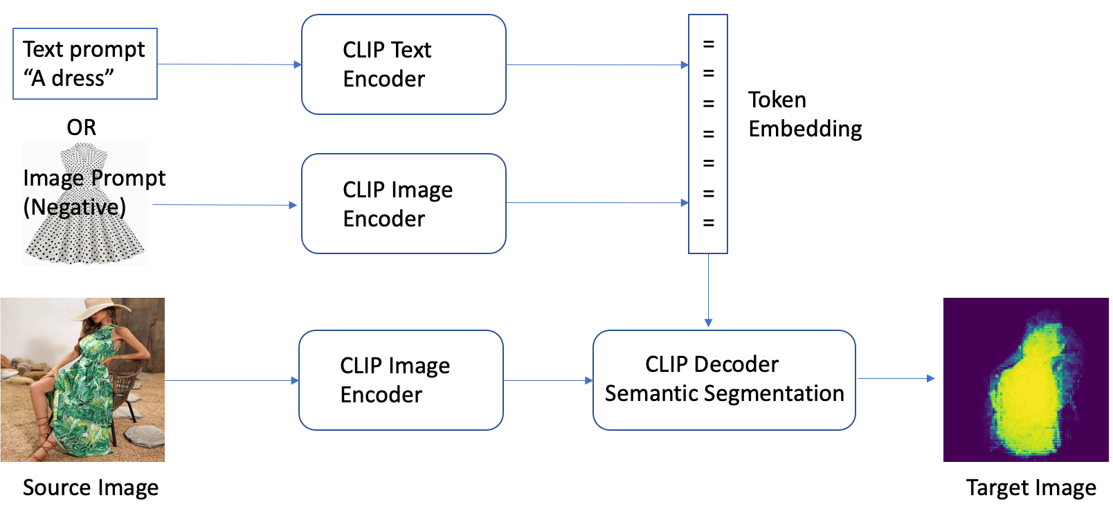
CLIPSeg is a model that uses a text and image encoder to encode textual and visual information into a multimodal embedding space to perform semantic segmentation based on a text prompt. The architecture of CLIPSeg consists of two main components: a text encoder and an image encoder. The text encoder takes in the text prompt and converts it into a text embedding, while the image encoder takes in the image and converts it into an image embedding. Both embeddings are then concatenated and passed through a fully connected layer to produce the final segmentation mask.

In terms of data flow, the model is trained on a dataset of images and corresponding text prompts, where the text prompts describe the target object to be segmented. During the training process, the text encoder and image encoder are optimized to learn the mapping between the text prompts and the image to produce the final segmentation mask. Once the model is trained, it can take in a new text prompt and image and produce a segmentation mask for the object described in the prompt.

Stable Diffusion is a technique that allows fashion designers to generate highly realistic imagery in large quantities purely based on text descriptions without the need for lengthy and expensive customization. This is beneficial for designers who want to create vogue styles quickly, and manufacturers who want to produce personalized products at a lower cost.

The following diagram illustrates the Stable Diffusion architecture and data flow.

Stable Diffusion Architecture

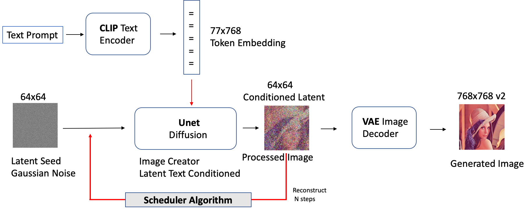
Compared to traditional GAN-based methods, Stable Diffusion is a generative AI that is capable of producing more stable and photo-realistic images that match the distribution of the original image. The model can be conditioned on a wide range of purposes, such as text for text-to-image generation, bounding boxes for layout-to-image generation, masked images for in-painting, and lower-resolution images for super-resolution. Diffusion models have a wide range of business applications, and their practical uses continue to evolve. These models will greatly benefit various industries such as fashion, retail and e-commerce, entertainment, social media, marketing, and more.

Generate masks from text prompts using CLIPSeg

Vogue online styling is a service that enables customers to receive fashion advice and recommendations from AI through an online platform. It does this by selecting clothing and accessories that complement the customer’s appearance, fit within their budget, and match their personal preferences. With the utilization of generative AI, tasks can be accomplished with greater ease, leading to increased customer satisfaction and reduced expenses.

The solution can be deployed on an Amazon Elastic Compute Cloud (EC2) p3.2xlarge instance, which has one single V100 GPU with 16G memory. Several techniques were employed to improve performance and reduce GPU memory usage, resulting in faster image generation. These include using fp16 and enabling memory efficient attention to decrease bandwidth in the attention block.

We began by having the user upload a fashion image, followed by downloading and extracting the pre-trained model from CLIPSeq. The image is then normalized and resized to comply with the size limit. Stable Diffusion V2 supports image resolution up to 768×768 while V1 supports up to 512×512. See the following code:

from models.clipseg import CLIPDensePredT

# The original image
image = download_image(img_url).resize((768, 768))

# Download pre-trained CLIPSeq model and unzip the pkg
! wget https://owncloud.gwdg.de/index.php/s/ioHbRzFx6th32hn/download -O weights.zip
! unzip -d weights -j weights.zip

# Load CLIP model. Available models = ['RN50', 'RN101', 'RN50x4', 
# 'RN50x16', 'RN50x64', 'ViT-B/32', 'ViT-B/16', 'ViT-L/14', 'ViT-L/14@336px']
model = CLIPDensePredT(version='ViT-B/16', reduce_dim=64)
model.eval()

# non-strict, because we only stored decoder weights (not CLIP weights)
model.load_state_dict(torch.load('weights/rd64-uni.pth', 
    map_location=torch.device('cuda')), strict=False)

# Image normalization and resizing
transform = transforms.Compose([
    transforms.ToTensor(),
    transforms.Normalize(mean=[0.485, 0.456, 0.406], std=[0.229, 0.224, 0.225]),
    transforms.Resize((768, 768)),
])
img = transform(image).unsqueeze(0)

With the use of the pre-trained CLIPSeq model, we are able to extract the target object from an image using a text prompt. This is done by inputting the text prompt into the text encoder, which converts it into a text embedding. The image is then input into the image encoder, which converts it into an image embedding. Both embeddings are then concatenated and passed through a fully connected layer to produce the final segmentation mask, which highlights the target object described in the text prompt. See the following code:

# Text prompt
prompt = 'Get the dress only.'

# predict
mask_image_filename = 'the_mask_image.png'
with torch.no_grad():
    preds = model(img.repeat(4,1,1,1), prompt)[0]
    
# save the mask image after computing the area under the standard 
#   Gaussian probability density function and calculates the cumulative 
#   distribution function of the normal distribution with ndtr.   
plt.imsave(mask_image_filename,torch.special.ndtr(preds[0][0]))

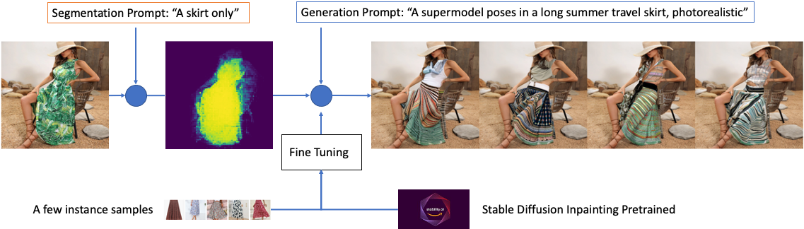
With the accurate mask image from semantic segmentation, we can use in-painting for content substitution. In-painting is the process of using a trained generative model to fill in missing parts of an image. By using the mask image to identify the target object, we can apply the in-painting technique to substitute the target object with something else, such as a different clothing item or accessory. The Stable Diffusion V2 model can be used for this purpose, because it is capable of producing high-resolution, photo-realistic images that match the distribution of the original image.

Fine-tuning from pre-trained models using DreamBooth

Fine-tuning is a process in deep learning where a pre-trained model is further trained on a new task using a small amount of labelled data. Rather than training from scratch, the idea is to take a network that has already been trained on a large dataset for a similar task and further train it on a new dataset to make it more specialized for that particular task.

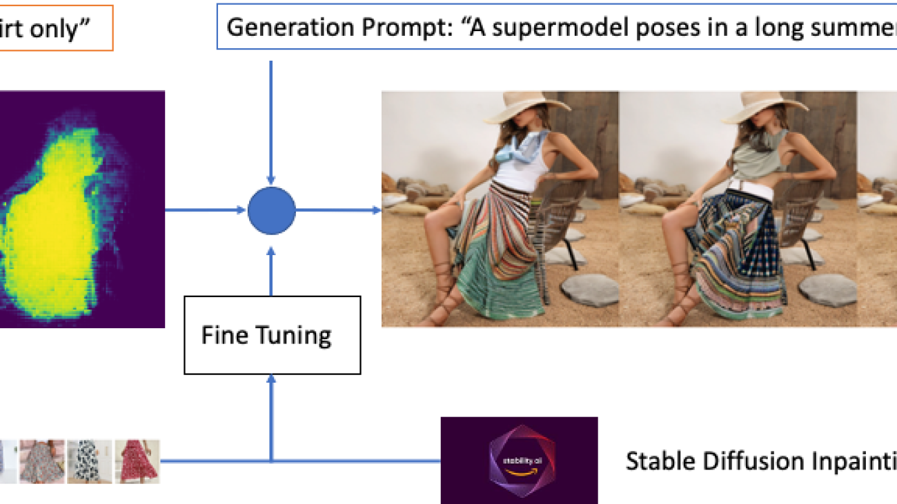
Fashion designers can also use a subject-driven, fine-tuned Stable Diffusion in-painting model to generate a specific class of style, such as casual long skirts for ladies. To do this, the first step is to provide a set of sample images in the target domain, roughly about 1 dozens, with proper text labels such as the following and binding them to a unique identifier that references the design, style, color and fabric. The label on the text plays a critical role in determining the results of the fine-tuned model. There are several ways to enhance fine tuning through effective prompt engineering and here are a few examples.

Sample text prompts to descibe some of the most common design elements of casual 
long skirts for ladies:

Design Style: A-line, wrap, maxi, mini, and pleated skirts are some of the most 
    popular styles for casual wear. A-line skirts are fitted at the waist and 
    flare out at the hem, creating a flattering silhouette. Wrap skirts have a
    wrap closure and can be tied at the waist for a customizable fit. Maxi skirts 
    are long and flowy, while mini skirts are short and flirty. Pleated skirts 
    have folds that add texture and movement to the garment.
Pattern: Casual skirts can feature a variety of patterns, including stripes, 
    florals, polka dots, and solids. These patterns can range from bold and graphic 
    to subtle and understated.
Colors: Casual skirts come in a range of colors, including neutral shades likeblack, 
    white, and gray, as well as brighter hues like pink, red, and blue. Some skirts 
    may also feature multiple colors in a single garment, such asa skirt with a bold 
    pattern that incorporates several shades.
Fabrics: Common fabrics used in casual skirts include cotton, denim, linen, and 
    rayon. These materials offer different levels of comfort and durability, making 
    it easy to find a skirt that suits your personal style and needs.

Using a small set of images to fine-tune Stable Diffusion may result in model overfitting. DreamBooth[5] addresses this by using a class-specific prior-preservation loss. It learns to bind a unique identifier with that specific subject in two steps. First, it fine-tunes the low-resolution model with the input images paired with a text prompt that contains a unique identifier and the name of the class the subject belongs to, such as “skirt”. In practice, this means having the model fit images and the images sampled from the visual prior of the non-fine-tuned class simultaneously. These prior-preserving images are sampled and labeled using the “class noun” prompt. Second, it will fine-tune the super-high-resolution components by pairing low-resolution and high-resolution images from the input images set, which allows the outputs of the fine-tuned model to maintain fidelity to small details.

Fine-tuning a pre-trained in-painting text encoder with the UNet for resolution 512×512 images requires approximately 22GB of VRAM or higher for 768×768 resolution.  Ideally fine-tune samples should be resized to match the desirable output image resolution to avoid performance degradation. The text encoder produces more accurate details such as model faces. One option is to run on a single AWS EC2 g5.2xlarge instance, now available in eight regions or use Hugging Face Accelerate to run the fine-tuned code across a distributed configuration. For additional memory savings, you can choose a sliced version of attention that performs the computation in steps instead of all at once by simply modifying DreamBooth’s training script train_dreambooth_inpaint.py to add the pipeline enable_attention_slicing() function.

Accelerate is a library that enables one fine tuning code to be run across any distributed configuration. Hugging Face and Amazon introduced Hugging Face Deep Learning Containers (DLCs) to scale fine tuning tasks across multiple GPUs and nodes. You can configure the launch configuration for Amazon SageMaker with a single CLI command.

# From your aws account, install the sagemaker sdk for Accelerate
pip install "accelerate[sagemaker]" --upgrade

# Configure the launch configuration for Amazon SageMaker 
accelerate config

# List and verify Accelerate configuration
accelerate env

# Make necessary modification of the training script as the following to save 
# output on S3, if needed
#  - torch.save('/opt/ml/model`)
#  + accelerator.save('/opt/ml/model')

To launch a fine-tune job, verify Accelerate’s configuration using CLI and provide the necessary training arguments, then use the following shell script.

# Instance images — Custom images that represents the specific 
#          concept for dreambooth training. You should collect 
#          high #quality images based on your use cases.
# Class images — Regularization images for prior-preservation 
#          loss to prevent overfitting. You should generate these 
#          images directly from the base pre-trained model. 
#          You can choose to generate them on your own or generate 
#         them on the fly when running the training script.
# 
# You can access train_dreambooth_inpaint.py from huggingface/diffuser 

export MODEL_NAME="stabilityai/stable-diffusion-2-inpainting"
export INSTANCE_DIR="/data/fashion/gowns/highres/"
export CLASS_DIR="/opt/data/fashion/generated_gowns/imgs"
export OUTPUT_DIR="/opt/model/diffuser/outputs/inpainting/"

accelerate launch train_dreambooth_inpaint.py 
  --pretrained_model_name_or_path=$MODEL_NAME  
  --train_text_encoder 
  --instance_data_dir=$INSTANCE_DIR 
  --class_data_dir=$CLASS_DIR 
  --output_dir=$OUTPUT_DIR 
  --with_prior_preservation --prior_loss_weight=1.0 
  --instance_prompt="A supermodel poses in long summer travel skirt, photorealistic" 
  --class_prompt="A supermodel poses in skirt, photorealistic" 
  --resolution=512 
  --train_batch_size=1 
  --use_8bit_adam 
  --gradient_checkpointing 
  --learning_rate=2e-6 
  --lr_scheduler="constant" 
  --lr_warmup_steps=0 
  --num_class_images=200 
  --max_train_steps=800

The fine-tuned in-painting model allows for the generation of more specific images to the fashion class described by the text prompt. Because it has been fine-tuned with a set of high-resolution images and text prompts, the model can generate images that are more tailored to the class, such as formal evening gowns. It’s important to note that the more specific the class and the more data used for fine-tuning, the more accurate and realistic the output images will be.

%tree -d ./finetuned-stable-diffusion-v2-1-inpainting
finetuned-stable-diffusion-v2-1-inpainting
├── 512-inpainting-ema.ckpt
├── feature_extractor
├── code
│ └──inference.py
│ ├──requirements.txt
├── scheduler
├── text_encoder 
├── tokenizer
├── unet
└── vae

Deploy a fine-tuned in-painting model using SageMaker for inference

With Amazon SageMaker, you can deploy the fine-tuned Stable Diffusion models for real-tim inference. To upload the model to Amazon Simple Storage service (S3) for deployment, a model.tar.gz archive tarball must be created. Ensure the archive directly includes all files, not a folder that contains them. The DreamBooth fine-tuning archive folder should appear as follows after eliminating the intermittent checkpoints:

The initial step in creating our inference handler involves the creation of the inference.py file. This file serves as the central hub for loading the model and handling all incoming inference requests. After the model is loaded, the model_fn() function is executed. When the need arises to perform inference, the predict_fn() function is called. Additionally, the decode_base64() function is utilized to convert a JSON string, contained within the payload, into a PIL image data type.

%%writefile code/inference.py
import base64
import torch
from PIL import Image
from io import BytesIO
from diffusers import EulerDiscreteScheduler, StableDiffusionInpaintPipeline

def decode_base64(base64_string):
    decoded_string = BytesIO(base64.b64decode(base64_string))
    img = Image.open(decoded_string)
    return img

def model_fn(model_dir):
    # Load stable diffusion and move it to the GPU
    scheduler = EulerDiscreteScheduler.from_pretrained(model_dir, subfolder="scheduler")
    pipe = StableDiffusionInpaintPipeline.from_pretrained(model_dir, 
                                                   scheduler=scheduler,
                                                   revision="fp16",
                                                   torch_dtype=torch.float16)
    pipe = pipe.to("cuda")
    pipe.enable_xformers_memory_efficient_attention()
    #pipe.enable_attention_slicing()
    return pipe


def predict_fn(data, pipe):
    # get prompt & parameters
    prompt = data.pop("inputs", data) 
    # Require json string input. Inference to convert imge to string.
    input_img = data.pop("input_img", data)
    mask_img = data.pop("mask_img", data)
    # set valid HP for stable diffusion
    num_inference_steps = data.pop("num_inference_steps", 25)
    guidance_scale = data.pop("guidance_scale", 6.5)
    num_images_per_prompt = data.pop("num_images_per_prompt", 2)
    image_length = data.pop("image_length", 512)
    # run generation with parameters
    generated_images = pipe(
        prompt,
        image = decode_base64(input_img),
        mask_image = decode_base64(mask_img),
        num_inference_steps=num_inference_steps,
        guidance_scale=guidance_scale,
        num_images_per_prompt=num_images_per_prompt,
        height=image_length,
        width=image_length,
    #)["images"] # for Stabel Diffusion v1.x
    ).images
    
    # create response
    encoded_images = []
    for image in generated_images:
        buffered = BytesIO()
        image.save(buffered, format="JPEG")
        encoded_images.append(base64.b64encode(buffered.getvalue()).decode())
        
    return {"generated_images": encoded_images}

To upload the model to an Amazon S3 bucket, it’s necessary to first create a model.tar.gz archive. It’s crucial to note that the archive should consist of the files directly and not a folder that holds them. For instance, the file should appear as follows:

import tarfile
import os

# helper to create the model.tar.gz
def compress(tar_dir=None,output_file="model.tar.gz"):
    parent_dir=os.getcwd()
    os.chdir(tar_dir)
    with tarfile.open(os.path.join(parent_dir, output_file), "w:gz") as tar:
        for item in os.listdir('.'):
          print(item)
          tar.add(item, arcname=item)    
    os.chdir(parent_dir)
            
compress(str(model_tar))

# After we created the model.tar.gz archive we can upload it to Amazon S3. We will 
# use the sagemaker SDK to upload the model to our sagemaker session bucket.
from sagemaker.s3 import S3Uploader

# upload model.tar.gz to s3
s3_model_uri=S3Uploader.upload(local_path="model.tar.gz", 
        desired_s3_uri=f"s3://{sess.default_bucket()}/finetuned-stable-diffusion-v2-1-inpainting")

After the model archive is uploaded, we can deploy it on Amazon SageMaker using HuggingfaceModel for real-time inference. You can host the endpoint using a g4dn.xlarge instance, which is equipped with a single NVIDIA Tesla T4 GPU with 16GB of VRAM. Autoscaling can be activated to handle varying traffic demands. For information on incorporating autoscaling in your endpoint, see Going Production: Auto-scaling Hugging Face Transformers with Amazon SageMaker.

from sagemaker.huggingface.model import HuggingFaceModel

# create Hugging Face Model Class
huggingface_model = HuggingFaceModel(
   model_data=s3_model_uri,      # path to your model and script
   role=role,                    # iam role with permissions to create an Endpoint
   transformers_version="4.17",  # transformers version used
   pytorch_version="1.10",       # pytorch version used
   py_version='py38',            # python version used
)

# deploy the endpoint endpoint
predictor = huggingface_model.deploy(
    initial_instance_count=1,
    instance_type="ml.g4dn.xlarge"
    )

The huggingface_model.deploy() method returns a HuggingFacePredictor object that can be used to request inference. The endpoint requires a JSON with an inputs key, which represents the input prompt for the model to generate an image. You can also control the generation with parameters such as num_inference_steps, guidance_scale, and “num_images_per_prompt”. The predictor.predict() function returns a JSON with a “generated_images” key, which holds the four generated images as base64 encoded strings. We added two helper functions, decode_base64_to_image and display_images, to decode the response and display the images respectively. The former decodes the base64 encoded string and returns a PIL.Image object, and the latter displays a list of PIL.Image objects. See the following code:

import PIL
from io import BytesIO
from IPython.display import display
import base64
import matplotlib.pyplot as plt
import json

# Encoder to convert an image to json string
def encode_base64(file_name):
    with open(file_name, "rb") as image:
        image_string = base64.b64encode(bytearray(image.read())).decode()
    return image_string
    
# Decode to to convert a json str to an image 
def decode_base64_image(base64_string):
    decoded_string = BytesIO(base64.b64decode(base64_string))
    img = PIL.Image.open(decoded_string)
    return img
    
# display PIL images as grid
def display_images(images=None,columns=3, width=100, height=100):
    plt.figure(figsize=(width, height))
    for i, image in enumerate(images):
        plt.subplot(int(len(images) / columns + 1), columns, i + 1)
        plt.axis('off')
        plt.imshow(image)
        
# Display images in a row/col grid
def image_grid(imgs, rows, cols):
    assert len(imgs) == rows*cols
    w, h = imgs[0].size
    grid = PIL.Image.new('RGB', size=(cols*w, rows*h))
    grid_w, grid_h = grid.size
    
    for i, img in enumerate(imgs):
        grid.paste(img, box=(i%cols*w, i//cols*h))
    return grid

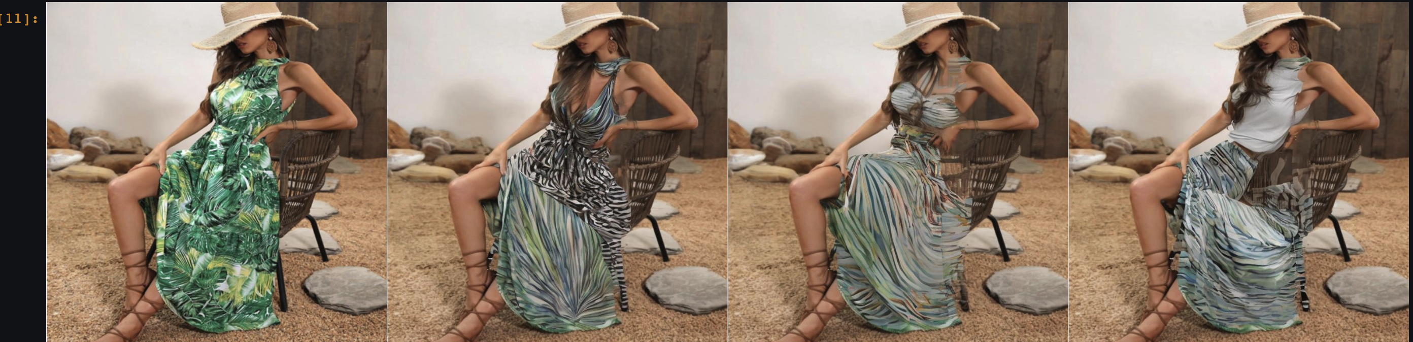
Let’s move forward with the in-painting task. It has been estimated that it will take roughly 15 seconds to produce three images, given the input image and the mask created using CLIPSeg with the text prompt discussed previously. See the following code:

num_images_per_prompt = 3
prompt = "A female super-model poses in a casual long vacation skirt, with full body length, bright colors, photorealistic, high quality, highly detailed, elegant, sharp focus"

# Convert image to string
input_image_filename = "./imgs/skirt-model-2.jpg"
encoded_input_image = encode_base64(input_image_filename)
encoded_mask_image = encode_base64("./imgs/skirt-model-2-mask.jpg")


# Set in-painint parameters
guidance_scale = 6.7
num_inference_steps = 45

# run prediction
response = predictor.predict(data={
  "inputs": prompt,
  "input_img": encoded_input_image,
  "mask_img": encoded_mask_image,
  "num_images_per_prompt" : num_images_per_prompt,
  "image_length": 768
  }
)

# decode images
decoded_images = [decode_base64_image(image) for image in response["generated_images"]]

# visualize generation
display_images(decoded_images, columns=num_images_per_prompt, width=100, height=100)

# insert initial image in the list so we can compare side by side
image = PIL.Image.open(input_image_filename).convert("RGB")
decoded_images.insert(0, image)
                       
# Display inpainting images in grid
image_grid(decoded_images, 1, num_images_per_prompt + 1)

The in-painted images can be displayed along with the original image for visual comparison. Additionally, the in-painting process can be constrained using various parameters such as guidance_scale, which controls the strength of the guidance image during the in-painting process. This allows the user to adjust the output image and achieve the desired results.
Inference Output

Amazon SageMaker Jumpstart offers Stable Diffusion templates for various models, including text-to-image and upscaling. For more information, please refer to SageMaker JumpStart now provides Stable Diffusion and Bloom models. Additional Jumpstart templates will be available in the near future.

Limitations

Although CLIPSeg usually performs well on recognizing common objects, it struggles on more abstract or systematic tasks such as counting the number of objects in an image and on more complex tasks such as predicting how close the nearest object such a handbag is in a photo. Zero-shot CLIPSeq also struggles compared to task-specific models on very fine-grained classification, such as telling the difference between two vague designs, variants of dress, or style classification. CLIPSeq also still has poor generalization to images not covered in its pre-training dataset. Finally, it has been observed that CLIP’s zero-shot classifiers can be sensitive to wording or phrasing and sometimes require trial and error “prompt engineering” to perform well. Switching to a different semantic segmentation model for CLIPSeq’s backbone, such as BEiT, which boasts a 62.8% mIOU on the ADE20K dataset, could potentially improve results.

Fashion designs generated by using Stable Diffusion have been found to be limited to parts of garments that are at least as predictably-placed in the wider context of the fashion models, and which conform to high-level embeddings that you could reasonably expect to find in a hyperscale dataset used during training the pre-trained model. The real limit of generative AI is that the model will eventually produce totally imaginary and less authentic outputs. Therefore, the fashion designs generated by AI may not be as varied or unique as those created by human designers.

Conclusion

Generative AI provides the fashion sector an opportunity to transform their practices through better user experiences and cost-efficient business strategies. In this post, we showcase how to harness generative AI to enable fashion designers and consumers to create personalized fashion styles using virtual modeling. With the assistance of existing Amazon SageMaker Jumpstart templates and those to come, users can quickly embrace these advanced techniques without needing in-depth technical expertise, all while maintaining versatility and lowering expenses.

This innovative technology presents new chances for companies and professionals involved in content generation, across various industries. Generative AI provides ample capabilities for enhancing and creating content. Try out the recent additions to the Jumpstart templates in your SageMaker Studio, such as fine-tuning text-to-image and upscale capabilities.

We would like to thank Li Zhang, Karl Albertsen, Kristine Pearce, Nikhil Velpanur, Aaron Sengstacken, James Wu and Neelam Koshiya for their supports and valuable inputs that helped improve this work.


About the Authors

Alfred Shen is a Senior AI/ML Specialist at AWS. He has been worked in Silicon Valley, holding technical and managerial positions in diverse sectors including healthcare, finance, and high-tech. He is a dedicated applied AI/ML researcher, concentrating on CV, NLP, and multimodality. His work has been showcased in publications such as EMNLP, ICLR, and Public Health.

Vivek MadanDr. Vivek Madan is an Applied Scientist with the Amazon SageMaker JumpStart team. He got his PhD from University of Illinois at Urbana-Champaign and was a Post Doctoral Researcher at Georgia Tech. He is an active researcher in machine learning and algorithm design and has published papers in EMNLP, ICLR, COLT, FOCS, and SODA conferences

Read More

How Kakao Games automates lifetime value prediction from game data using Amazon SageMaker and AWS Glue

How Kakao Games automates lifetime value prediction from game data using Amazon SageMaker and AWS Glue

This post is co-written with Suhyoung Kim, General Manager at KakaoGames Data Analytics Lab.

Kakao Games is a top video game publisher and developer headquartered in South Korea. It specializes in developing and publishing games on PC, mobile, and virtual reality (VR) serving globally. In order to maximize its players’ experience and improve the efficiency of operations and marketing, they are continuously adding new in-game items and providing promotions to their players. The result of these events can be evaluated afterwards so that they make better decisions in the future.

However, this approach is reactive. If we can forecast lifetime value (LTV), we can take a proactive approach. In other words, these activities can be planned and run based on the forecasted LTV, which determines the players’ values through their lifetime in the game. With this proactive approach, Kakao Games can launch the right events at the right time. If the forecasted LTV for some players is decreasing, this means that the players are likely to leave soon. Kakao Games can then create a promotional event not to leave the game. This makes it important to accurately forecast the LTV of their players. LTV is the measurement adopted by not only gaming companies but also any kind of service with long-term customer engagement. Statistical methods and machine learning (ML) methods are actively developed and adopted to maximize the LTV.

In this post, we share how Kakao Games and the Amazon Machine Learning Solutions Lab teamed up to build a scalable and reliable LTV prediction solution by using AWS data and ML services such as AWS Glue and Amazon SageMaker.

We chose one of the most popular games of Kakao Games, ODIN, as the target game for the project. ODIN is a popular massively multiplayer online roleplaying game (MMORPG) for PC and mobile devices published and operated by Kakao Games. It was launched in June 2021 and has been ranked within the top three in revenue in Korea.

Kakao Games ODIN

Challenges

In this section, we discuss challenges around various data sources, data drift caused by internal or external events, and solution reusability. These challenges are typically faced when we implement ML solutions and deploy them into a production environment.

Player behavior affected by internal and external events

It’s challenging to forecast the LTV accurately, because there are many dynamic factors affecting player behavior. These include game promotions, newly added items, holidays, banning accounts for abuse or illegal play, or unexpected external events like sport events or severe weather conditions. This means that the model working this month might not work well next month.

We can utilize external events as ML features along with the game-related logs and data. For example, Amazon Forecast supports related time series data like weather, prices, economic indicators, or promotions to reflect internal and external related events. Another approach is to refresh ML models regularly when data drift is observed. For our solution, we chose the latter method because the related event data wasn’t available and we weren’t sure how reliable the existing data was.

Continuous ML model retraining is one method to overcome this challenge by relearning from the most recent data. This requires not only well-designed features and ML architecture, but also data preparation and ML pipelines that can automate the retraining process. Otherwise, the ML solution can’t be efficiently operated in the production environment due to the complexity and poor repeatability.

It’s not sufficient to retrain the model using the latest training dataset. The retrained model might not give a more accurate forecasting result than the existing one, so we can’t simply replace the model with the new one without any evaluation. We need to be able to go back to the previous model if the new model starts to underperform for some reason.

To solve this problem, we had to design a strong data pipeline to create the ML features from the raw data and MLOps.

Multiple data sources

ODIN is an MMORPG where the game players interact with each other, and there are various events such as level-up, item purchase, and gold (game money) hunting. It produces about 300 GB logs every day from its more than 10 million players across the world. The gaming logs are of different types, such as player login, player activity, player purchases, and player level-ups. These types of data are historical raw data from an ML perspective. For example, each log is written in the format of timestamp, user ID, and event information. The interval of logs is not uniform. Also, there is static data describing the players such as their age and registration date, which is non-historical data. LTV prediction modeling requires these two types of data as its input because they complement each other to represent the player’s characteristics and behavior.

For this solution, we decided to define the tabular dataset combining the historical features with the fixed number of aggregated steps along with the static player features. The aggregated historical features are generated through multiple steps from the number of game logs, which are stored in Amazon Athena tables. In addition to the challenge of defining the features for the ML model, it’s critical to automate the feature generation process so that we can get ML features from the raw data for ML inference and model retraining.

To solve this problem, we build an extract, transform, and load (ETL) pipeline that can be run automatically and repeatedly for training and inference dataset creation.

Scalability to other games

Kakao Games has other games with long-term player engagements just like ODIN. Naturally, LTV prediction benefits those games as well. Because most of the games share similar log types, they want to reuse this ML solution to other games. We can fulfill this requirement by using the common log and attributes among different games when we design the ML model. But there is still an engineering challenge. The ETL pipeline, MLOps pipeline, and ML inference should be rebuilt in a different AWS account. Manual deployment of this complex solution isn’t scalable and the deployed solution is hard to maintain.

To solve this problem, we make the ML solution auto-deployable with a few configuration changes.

Solution overview

The ML solution for LTV forecasting is composed of four components: the training dataset ETL pipeline, MLOps pipeline, inference dataset ETL pipeline, and ML batch inference.

The training and inference ETL pipeline creates ML features from the game logs and the player’s metadata stored in Athena tables, and stores the resulting feature data in an Amazon Simple Storage Service (Amazon S3) bucket. ETL requires multiple transformation steps, and the workflow is implemented using AWS Glue. The MLOps trains ML models, evaluates the trained model against the existing model, and then registers the trained model to the model registry if it outperforms the existing model. These are all implemented as a single ML pipeline using Amazon SageMaker Pipelines, and all the ML trainings are managed via Amazon SageMaker Experiments. With SageMaker Experiments, ML engineers can find which training and evaluation datasets, hyperparameters, and configurations were used for each ML model during the training or later. ML engineers no longer need to manage this training metadata separately.

The last component is the ML batch inference, which is run regularly to predict LTV for the next couple of weeks.

The following figure shows how these components work together as a single ML solution.

ML Ops architecture

The solution architecture has been implemented using the AWS Cloud Development Kit (AWS CDK) to promote infrastructure as code (IaC), making it easy to version control and deploy the solution across different AWS accounts and Regions

In the following sections, we discuss each component in more detail.

Data pipeline for ML feature generation

Game logs stored in Athena backed by Amazon S3 go through the ETL pipelines created as Python shell jobs in AWS Glue. It enables running Python scripts with AWS Glue for feature exaction to generate the training-ready dataset. Corresponding tables in each phase are created in Athena. We use AWS Glue for running the ETL pipeline due to its serverless architecture and flexibility in generating different versions of the dataset by passing in various start and end dates. Refer to Accessing parameters using getResolvedOptions to learn more about how to pass the parameters to an AWS Glue job. With this method, the dataset can be created to cover a period of as short as 4 weeks, supporting the game in its early stages. For instance, the input start date and prediction start date for each version of dataset are parsed via the following code:

import sys
from awsglue.utils import getResolvedOptions

args = getResolvedOptions(
    sys.argv,
    [
        'JOB_NAME',
        'db_name',
        'ds_version',
        'input_start_date',
        'prediction_start_date',
        'bucket',
        'prefix',
        'timestamp'
    ]
)

AWS Glue jobs are designed and divided into different stages and triggered sequentially. Each job is configured to take in positional and key-value pair arguments to run customized ETL pipelines. One key parameter is the start and end date of the data that is used in training. This is because the start and end date of data likely span different holidays, and serve as a direct factor in determining the length of dataset. To observe this parameter’s impact on model performances, we created nine different dataset versions (with different start dates and length of training period).

Specifically, we created dataset versions with different start dates (shifted by 4 weeks) and different training periods (12 weeks, 16 weeks, 20 weeks, 24 weeks, and 28 weeks) in nine Athena databases backed by Amazon S3. Each version of the dataset contains the features describing player characteristics and in-game purchase activity time series data.

ML model

We selected AutoGluon for model training implemented with SageMaker pipelines. AutoGluon is a toolkit for automated machine learning (AutoML). It enables easy-to-use and easy-to-extend AutoML with a focus on automated stack ensembling, deep learning, and real-world applications spanning image, text, and tabular data.

You can use AutoGluon standalone to train ML models or in conjunction with Amazon SageMaker Autopilot, a feature of SageMaker that provides a fully managed environment for training and deploying ML models.

In general, you should use AutoGluon with Autopilot if you want to take advantage of the fully managed environment provided by SageMaker, including features such as automatic scaling and resource management, as well as easy deployment of trained models. This can be especially useful if you’re new to ML and want to focus on training and evaluating models without worrying about the underlying infrastructure.

You can also use AutoGluon standalone when you want to train ML models in a customized way. In our case, we used AutoGluon with SageMaker to realize a two-stage prediction, including churn classification and lifetime value regression. In this case, the players that stopped purchasing game items are considered as having churned.

Let’s talk about the modeling approach for LTV prediction and the effectiveness of the model retraining against the data drift symptom, which means the internal or external events that change a player’s purchase pattern.

First, the modeling processes were separated into two stages, including a binary classification (classifying a player as churned or not) and a regression model that was trained to predict the LTV value for non-churned players:

  • Stage 1 – Target values for LTV are converted into a binary label, LTV = 0 and LTV > 0. AutoGluon TabularPredictor is trained to maximize F1 score.
  • Stage 2 – A regression model using AutoGluon TabularPredictor is used to train the model on users with LTV > 0 for actual LTV regression.

During the model testing phase, the test data goes through the two models sequentially:

  • Stage 1 – The binary classification model runs on test data to get the binary prediction 0 (user having LTV = 0, churned) or 1 (user having LTV > 0, not churned).
  • Stage 2 – Players predicted with LTV > 0 go through the regression model to get the actual LTV value predicted. Combined with the user predicted as having LTV = 0, the final LTV prediction result is generated.

Model artifacts associated with the training configurations for each experiment and for each version of dataset are stored in an S3 bucket after the training, and also registered to the SageMaker Model Registry within the SageMaker Pipelines run.

To test if there is any data drift due to using the same model trained on the dataset v1 (12 weeks starting from October), we run inference on dataset v1, v2 (starting time shifted forward by 4 weeks), v3 (shifted forward by 8 weeks), and so on for v4 and v5. The following table summarizes model performance. The metric used for comparison is minmax score, whose range is 0–1. It gives a higher number when the LTV prediction is closer to the true LTV value.

Dataset Version Minmax Score Difference with v1
v1 0.68756
v2 0.65283 -0.03473
v3 0.66173 -0.02584
v4 0.69633 0.00877
v5 0.71533 0.02777

A performance drop is seen on dataset v2 and v3, which is consistent with the analysis performed on various modeling approaches having decreasing performance on dataset v2 and v3. For v4 and v5, the model shows equivalent performance, and even shows a slight improvement on v5 without model retraining. However, when comparing model v1 performance on dataset v5 (0.71533) vs. model v5 performance on dataset v5 (0.7599), model retraining is improving performance significantly.

Training pipeline

SageMaker Pipelines provides easy ways to compose, manage, and reuse ML workflows; select the best models for deploying into production; track the models automatically; and integrate CI/CD into ML pipelines.

In the training step, a SageMaker Estimator is constructed with the following code. Unlike the normal SageMaker Estimator to create a training job, we pass a SageMaker pipeline session to SageMaker_session instead of a SageMaker session:

from sagemaker.estimator import Estimator
from sagemaker.workflow.pipeline_context import PipelineSession

pipeline_session = PipelineSession()

ltv_train = Estimator(
    image_uri=image_uri,
    instance_type=instance_type,
    instance_count=1,
    output_path=output_path,
    base_job_name=f'{base_jobname_prefix}/train',
    role=role,
    source_dir=source_dir,
    entry_point=entry_point,
    sagemaker_session=pipeline_session,
    hyperparameters=hyperparameters
)

The base image is retrieved by the following code:

image_uri = SageMaker.image_uris.retrieve(
        "AutoGluon",
        region=region,
        version=framework_version,
        py_version=py_version,
        image_scope="training",
        instance_type=instance_type,
)

The trained model goes through the evaluation process, where the target metric is minmax. A score larger than the current best LTV minmax score will lead to a model register step, whereas a lower LTV minmax score won’t lead to the current registered model version being updated. The model evaluation on the holdout test dataset is implemented as a SageMaker Processing job.

The evaluation step is defined by the following code:

step_eval = ProcessingStep(
        name=f"EvaluateLTVModel-{ds_version}",
        processor=script_eval,
        inputs=[
            ProcessingInput(
                source=step_train.properties.ModelArtifacts.S3ModelArtifacts,
                destination="/opt/ml/processing/model",
            ),
            ProcessingInput(
                source=test,
                input_name='test',
                destination="/opt/ml/processing/test",
            ),
        ],
        outputs=[
            ProcessingOutput(output_name="evaluation", source="/opt/ml/processing/evaluation"),
        ],
        code=os.path.join(BASE_DIR, "evaluate_weekly.py"),
        property_files=[evaluation_report],
        job_arguments=["--test-fname", os.path.basename(test)],
    )

When the model evaluation is complete, we need to compare the evaluation result (minmax) with the existing model’s performance. We define another pipeline step, step_cond.

With all the necessary steps defined, the ML pipeline can be constructed and run with the following code:

# training pipeline
training_pipeline = Pipeline(
    name=f'odin-ltv-{ds_version}', 
    parameters=[
        processing_instance_count,
        model_approval_status,
        dataset_version,
        train_data,
        test_data,
        output_path,
        batch_instance_types,
        model_metrics,
        best_ltv_minmax_score
    ],
    steps=[step_train, step_eval, step_cond]
)

### start execution
execution = training_pipeline.start(
    parameters=dict(
        DatasetVersion=ds_version,
    )
)

The whole workflow is trackable and visualized in Amazon SageMaker Studio, as shown in the following graph. The ML training jobs are tracked by the SageMaker Experiment automatically so that you can find the ML training configuration, hyperparameters, dataset, and trained model of each training job. Choose each of the modules, logs, parameters, output, and so on to examine them in detail.

SaegMaker Pipelines

Automated batch inference

In the case of LTV prediction, batch inference is preferred to real-time inference because the predicted LTV is used for the offline downstream tasks normally. Just like creating ML features from the training dataset through the multi-step ETL, we have to create the ML features as an input to the LTV prediction model. We reuse the same workflow of AWS Glue to convert the players’ data into the ML features, but the data split and the label generation are not performed. The resulting ML feature is stored in the designated S3 bucket, which is monitored by an AWS Lambda trigger. When the ML feature file is dropped into the S3 bucket, the Lambda function runs automatically, which starts the SageMaker batch transform job using the latest and approved LTV model found in the SageMaker Model Registry. When the batch transform is complete, the output or predicted LTV values for each player are saved to the S3 bucket so that any downstream task can pick up the result. This architecture is described in the following diagram.

Data ETL pipeline

With this pipeline combining the ETL task and the batch inference, the LTV prediction is done simply running the AWS Glue ETL workflow regularly, such as once a week or once a month. AWS Glue and SageMaker manage their underlying resources, which means that this pipeline doesn’t require you to keep any resource running all the time. Therefore, this architecture using managed services is cost effective for batch tasks.

Deployable solution using the AWS CDK

The ML pipeline itself is defined and run using Pipelines, but the data pipeline and the ML model inference code including the Lambda function are out of the scope of Pipelines. To make this solution deployable so that we can apply this to other games, we defined the data pipeline and ML model inference using the AWS CDK. This way, the engineering team and data science team have the flexibility to manage, update, and control the whole ML solution without having to manage the infrastructure manually using the AWS Management Console.

Conclusion

In this post, we discussed how we could solve data drift and complex ETL challenges by building an automated data pipeline and ML pipeline utilizing managed services such as AWS Glue and SageMaker, and how to make it a scalable and repeatable ML solution to be adopted by other games using the AWS CDK.

“In this era, games are more than just content. They bring people together and have boundless potential and value when it comes to enjoying our lives. At Kakao Games, we dream of a world filled with games anyone can easily enjoy. We strive to create experiences where players want to stay playing and create bonds through community. The MLSL team helped us build a scalable LTV prediction ML solution using AutoGluon for AutoML, Amazon SageMaker for MLOps, and AWS Glue for data pipeline. This solution automates the model retraining for data or game changes, and can easily be deployed to other games via the AWS CDK. This solution helps us optimize our business processes, which in turn helps us stay ahead in the game.”

SuHyung Kim, Head of Data Analytics Lab, Kakao Games.

To learn more about related features of SageMaker and the AWS CDK, check out the following:

Amazon ML Solutions Lab

The Amazon ML Solutions Lab pairs your team with ML experts to help you identify and implement your organization’s highest-value ML opportunities. If you want to accelerate your use of ML in your products and processes, please contact the Amazon ML Solutions Lab.


About the Authors

Suhyoung Kim is a General Manager at KakaoGames Data Analytics Lab. He is responsible for gathering and analyzing data, and especially concern for the economy of online games.

Muhyun Kim is a data scientist at Amazon Machine Learning Solutions Lab. He solves customer’s various business problems by applying machine learning and deep learning, and also helps them gets skilled.

Sheldon Liu is a Data Scientist at Amazon Machine Learning Solutions Lab. As an experienced machine learning professional skilled in architecting scalable and reliable solutions, he works with enterprise customers to address their business problems and deliver effective ML solutions.

Alex Chirayath is a Senior Machine Learning Engineer at the Amazon ML Solutions Lab. He leads teams of data scientists and engineers to build AI applications to address business needs.

Gonsoo Moon, AI/ML Specialist Solutions Architect at AWS, has worked together customers to solve their ML problems using AWS AI/ML services. In the past, he had experience in developing machine learning services in the manufacture industry as well as in a large scale of service development, data analysis and system development in the portal and gaming industry. In his spare time, Gonsoo takes a walk and plays with children.

Read More