We’ve implemented initial support for plugins in ChatGPT. Plugins are tools designed specifically for language models with safety as a core principle, and help ChatGPT access up-to-date information, run computations, or use third-party services.OpenAI Blog

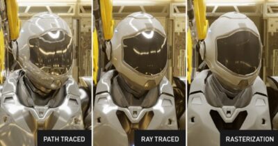
‘Cyberpunk 2077’ Brings Beautiful Path-Traced Visuals to GDC
Game developer CD PROJEKT RED today at the Game Developers Conference in San Francisco unveiled a technology preview for Cyberpunk 2077 with path tracing, coming April 11.
Path tracing, also known as full ray tracing, accurately simulates light throughout an entire scene. It’s used by visual effects artists to create film and TV graphics that are indistinguishable from reality. But until the arrival of GeForce RTX GPUs with RT Cores, and the AI-powered acceleration of NVIDIA DLSS, real-time video game path tracing was impossible because it is extremely GPU intensive.
“This not only gives better visuals to the players but also has the promise to revolutionize the entire pipeline of how games are being created,” said Pawel Kozlowski, a senior technology developer engineer at NVIDIA.
This technology preview, Cyberpunk 2077’s Ray Tracing: Overdrive Mode, is a sneak peak into the future of full ray tracing. With full ray tracing, now practically all light sources cast physically correct soft shadows. Natural colored lighting also bounces multiple times throughout Cyberpunk 2077’s world, creating more realistic indirect lighting and occlusion.
Cyberpunk 2077, previously an early adopter of ray tracing, becomes the latest modern blockbuster title to harness real-time path tracing. Coming shortly after path tracing for Minecraft, Portal and Quake II, it underscores a wave of adoption in motion.
Like with ray tracing, it’s expected many more will follow. And the influence on video games is just the start, as real-time path tracing holds promise for many design industries.
Decades of Research Uncorked
Decades in the making, real-time path tracing is indeed a big leap in gaming graphics.
While long used in computer-generated imagery for movies, path tracing there took place in offline rendering farms, often requiring hours to render a single frame.
In gaming, which requires fast frame rates, rendering needs to happen in about 0.016 seconds.
Since the 1970s, video games have relied on rasterization techniques (see below). More recently, in 2018, NVIDIA introduced RTX GPUs to support ray tracing. Path tracing is the final frontier for the most physically accurate lighting and shadows.
Path tracing has been one of the main lighting algorithms used in offline rendering farms and computer graphics in films for years. It wasn’t until GeForce RTX 40 series and DLSS 3 was available that it was possible to bring path tracing to real-time graphics.
Cyberpunk 2077 also taps into Shader Execution Reordering — available for use on the NVIDIA Ada Lovelace architecture generation — which optimizes GPU workloads, enabling more efficient path-traced lighting.
Accelerated by DLSS 3
DLSS 3 complements groundbreaking advancements in path tracing and harnesses modern AI — built on GPU-accelerated deep learning, a form of neural networking — as a powerful gaming performance multiplier. DLSS allows games to render 1/8th of the pixels, then uses AI and GeForce RTX Tensor Cores to reconstruct the rest, dramatically multiplying frame rates, while delivering crisp, high-quality images that rival native resolution.
Running on Ada Lovelace advances — launched with GeForce RTX 40 Series GPUs — DLSS 3 multiplies frame rates, maintaining image quality and responsiveness in games.
Powerful Tools Now Available
For game developers, NVIDIA today at GDC announced the availability of the RTX+ Path Tracing SDK 1.0. The package of technologies includes DLSS 3, Shader Execution Reordering (SER), RTX Direct Illumination (RTXDI) and NVIDIA Real-Time Denoisers (NRD).
Learn more about full RTX path tracing.
And catch up on all the breakthroughs in generative AI and the metaverse by joining us at GTC this week.

A Revolution Rendered in Real Time: NVIDIA Accelerates Neural Graphics at GDC
Gamers wanted better graphics. GPUs delivered. Those GPUs became the key to the world-changing AI revolution. Now gamers are reaping the benefits.
At GDC 2023 in San Francisco this week, the gaming industry’s premier developers conference, NVIDIA made a series of announcements, including new games and game development tools that promise to accelerate innovations at the intersection of neural networking and graphics, or neural graphics revolution.
DLSS 3 harnesses modern AI — built on GPU-accelerated deep learning, a form of neural networking — as a powerful gaming performance multiplier. DLSS allows games to render 1/8th of the pixels, then uses AI and GeForce RTX Tensor Cores to reconstruct the rest, dramatically multiplying frame rates, while delivering crisp, high-quality images that rival native resolution.
It’s just one example of how gamers are benefiting from the advancements in AI supercomputing showcased at this week’s NVIDIA GTC technology conference, which is running concurrently with GDC. And game developers are adopting DLSS at a break-neck pace.
DLSS complements ground-breaking advancements in ray tracing — a technology long used by filmmakers — to bring richer, more immersive visual experiences to gamers in real time.
Thanks, in part, to DLSS, real-time ray tracing, considered by many to be impossible in 2017, exploded onto the gaming scene with the debut of NVIDIA RTX in 2018. Ray tracing is now everywhere in games.
At GDC, game developer CD PROJEKT RED announced Cyberpunk 2077 will activate full ray tracing, also called path tracing, with the upcoming technology preview of Ray Tracing: Overdrive Mode in Cyberpunk 2077.
Cyberpunk 2077, previously an early adopter of ray tracing, becomes the latest modern blockbuster title to harness real-time path tracing following Minecraft, Portal and Quake II.
New DLSS 3 AAA Games Coming
During GDC, NVIDIA also announced the addition of DLSS 3 support for even more popular AAA games, including Diablo IV, Forza Horizon 5 and Redfall.
- Diablo IV, the latest installment of the genre-defining Diablo franchise with multiple games, will launch on June 6 with DLSS 3, with ray tracing coming post-launch.
- Forza Horizon 5, named the best open-world racing game of all time, will update to DLSS 3 on March 28.
- Redfall, Bethesda’s highly anticipated, open-world, co-op first-person shooter from Arkane Austin is launching on May 2 with DLSS 3, with ray tracing coming post-launch.
DLSS is now available in 270+ games and apps, and DLSS 3 is multiplying performance in 28 released games and has been adopted 7x faster than DLSS 2 in the first six months of their respective launches.
DLSS Frame Generation Now Publicly Available for Developers
NVIDIA announced DLSS Frame Generation is now publicly available for developers to integrate into their games and applications.
The public release of DLSS Frame Generation plug-ins will allow even more developers to adopt the framerate-boosting technology.
DLSS Frame Generation is now available via NVIDIA Streamline, an open-source, cross-vendor framework that simplifies the integration of super-resolution technologies in 3D games and apps.
For all the details, dig into our full coverage on GeForce News.
Unreal Engine 5.2 Integration to Speed Up DLSS 3 Adoption
At GDC, NVIDIA and Epic announced the integration of DLSS 3 into the popular Unreal Engine game engine.
Unreal Engine is an open and advanced real-time 3D creation tool that gives game developers and creators the freedom and control to deliver cutting-edge 3D content, interactive experiences and immersive virtual worlds.
A DLSS 3 plug-in will debut in UE 5.2, making it more straightforward for any developer to accelerate the performance of their games and applications, further accelerating the adoption of DLSS.
Cyberpunk 2077: A Showcase for What’s Next

CD PROJEKT RED showcases a technology preview of path tracing with Cyberpunk 2077.
Path tracing, also known as full ray tracing, allows developers to create cinematic experiences. Simulating the physics of light, using ray tracing as part of a neural graphics system, it’s capable of photorealism in 3D settings for more dynamic lighting and shadows.
GeForce gamers will be able to activate full ray tracing with the upcoming technology preview of Ray Tracing: Overdrive Mode on April 11.
These advancements are anchored in NVIDIA RTX technologies. To bring these incredible effects to life, CD PROJEKT RED and NVIDIA have worked hand in hand to integrate NVIDIA DLSS 3 and introduce new optimizations for this entirely new, fully ray-traced pipeline.
NVIDIA Shader Execution Reordering helps GPUs execute incoherent workloads boosting performance; NVIDIA Real-Time Denoisers have been used to improve performance and image quality.
As a result, with full ray tracing, now practically all light sources cast physically correct soft shadows. Natural colored lighting also bounces multiple times throughout Cyberpunk 2077’s world, creating more realistic indirect lighting and occlusion.
More to Come
Cyberpunk 2077 is a case study of how GPUs have unlocked the AI revolution and will bring great experiences to PC gamers for years to come.
An expanding game roster, game engine support and continued improvements in performance and image quality are securing NVIDIA DLSS as a landmark technology for the neural graphics revolution in PC gaming.

AI Opener: OpenAI’s Sutskever in Conversation With Jensen Huang
Like old friends catching up over coffee, two industry icons reflected on how modern AI got its start, where it’s at today and where it needs to go next.
Jensen Huang, founder and CEO of NVIDIA, interviewed AI pioneer Ilya Sutskever in a fireside chat at GTC. The talk was recorded a day after the launch of GPT-4, the most powerful AI model to date from OpenAI, the research company Sutskever co-founded.
They talked at length about GPT-4 and its forerunners, including ChatGPT. That generative AI model, though only a few months old, is already the most popular computer application in history.
Their conversation touched on the capabilities, limits and inner workings of the deep neural networks that are capturing the imaginations of hundreds of millions of users.
Compared to ChatGPT, GPT-4 marks a “pretty substantial improvement across many dimensions,” said Sutskever, noting the new model can read images as well as text.
“In some future version, [users] might get a diagram back” in response to a query, he said.
Under the Hood With GPT
“There’s a misunderstanding that ChatGPT is one large language model, but there’s a system around it,” said Huang.
In a sign of that complexity, Sutskever said OpenAI uses two levels of training.
The first stage focuses on accurately predicting the next word in a series. Here, “what the neural net learns is some representation of the process that produced the text, and that’s a projection of the world,” he said.
The second “is where we communicate to the neural network what we want, including guardrails … so it becomes more reliable and precise,” he added.
Present at the Creation
While he’s at the swirling center of modern AI today, Sutskever was also present at its creation.
In 2012, he was among the first to show the power of deep neural networks trained on massive datasets. In an academic contest, the AlexNet model he demonstrated with AI pioneers Geoff Hinton and Alex Krizhevsky recognized images faster than a human could.
Huang referred to their work as the Big Bang of AI.
The results “broke the record by such a large margin, it was clear there was a discontinuity here,” Huang said.
The Power of Parallel Processing
Part of that breakthrough came from the parallel processing the team applied to its model with GPUs.
“The ImageNet dataset and a convolutional neural network were a great fit for GPUs that made it unbelievably fast to train something unprecedented,” Sutskever said.

That early work ran on a few GeForce GTX 5080 GPUs in a University of Toronto lab. Today, tens of thousands of the latest NVIDIA A100 and H100 Tensor Core GPUs in the Microsoft Azure cloud service handle training and inference on models like ChatGPT.
“In the 10 years we’ve known each other, the models you’ve trained [have grown by] about a million times,” Huang said. “No one in computer science would have believed the computation done in that time would be a million times larger.”
“I had a very strong belief that bigger is better, and a goal at OpenAI was to scale,” said Sutskever.
A Billion Words
Along the way, the two shared a laugh.
“Humans hear a billion words in a lifetime,” Sutskever said.
“Does that include the words in my own head,” Huang shot back.
“Make it 2 billion,” Sutskever deadpanned.
The Future of AI
They ended their nearly hour-long talk discussing the outlook for AI.
Asked if GPT-4 has reasoning capabilities, Sutskever suggested the term is hard to define and the capability may still be on the horizon.
“We’ll keep seeing systems that astound us with what they can do,” he said. “The frontier is in reliability, getting to a point where we can trust what it can do, and that if it doesn’t know something, it says so,” he added.
“Your body of work is incredible … truly remarkable,” said Huang in closing the session. “This has been one of the best beyond Ph.D. descriptions of the state of the art of large language models,” he said.
To get all the news from GTC, watch the keynote below.
Automate Amazon Rekognition Custom Labels model training and deployment using AWS Step Functions
With Amazon Rekognition Custom Labels, you can have Amazon Rekognition train a custom model for object detection or image classification specific to your business needs. For example, Rekognition Custom Labels can find your logo in social media posts, identify your products on store shelves, classify machine parts in an assembly line, distinguish healthy and infected plants, or detect animated characters in videos.
Developing a Rekognition Custom Labels model to analyze images is a significant undertaking that requires time, expertise, and resources, often taking months to complete. Additionally, it often requires thousands or tens of thousands of hand-labeled images to provide the model with enough data to accurately make decisions. Generating this data can take months to gather and require large teams of labelers to prepare it for use in machine learning (ML).
With Rekognition Custom Labels, we take care of the heavy lifting for you. Rekognition Custom Labels builds off of the existing capabilities of Amazon Rekognition, which is already trained on tens of millions of images across many categories. Instead of thousands of images, you simply need to upload a small set of training images (typically a few hundred images or less) that are specific to your use case via our easy-to-use console. If your images are already labeled, Amazon Rekognition can begin training in just a few clicks. If not, you can label them directly within the Amazon Rekognition labeling interface, or use Amazon SageMaker Ground Truth to label them for you. After Amazon Rekognition begins training from your image set, it produces a custom image analysis model for you in just a few hours. Behind the scenes, Rekognition Custom Labels automatically loads and inspects the training data, selects the right ML algorithms, trains a model, and provides model performance metrics. You can then use your custom model via the Rekognition Custom Labels API and integrate it into your applications.
However, building a Rekognition Custom Labels model and hosting it for real-time predictions involves several steps: creating a project, creating the training and validation datasets, training the model, evaluating the model, and then creating an endpoint. After the model is deployed for inference, you might have to retrain the model when new data becomes available or if feedback is received from real-world inference. Automating the whole workflow can help reduce manual work.
In this post, we show how you can use AWS Step Functions to build and automate the workflow. Step Functions is a visual workflow service that helps developers use AWS services to build distributed applications, automate processes, orchestrate microservices, and create data and ML pipelines.
Solution overview
The Step Functions workflow is as follows:
- We first create an Amazon Rekognition project.
- In parallel, we create the training and the validation datasets using existing datasets. We can use the following methods:
- Import a folder structure from Amazon Simple Storage Service (Amazon S3) with the folders representing the labels.
- Use a local computer.
- Use Ground Truth.
- Create a dataset using an existing dataset with the AWS SDK.
- Create a dataset with a manifest file with the AWS SDK.
- After the datasets are created, we train a Custom Labels model using the CreateProjectVersion API. This could take from minutes to hours to complete.
- After the model is trained, we evaluate the model using the F1 score output from the previous step. We use the F1 score as our evaluation metric because it provides a balance between precision and recall. You can also use precision or recall as your model evaluation metrics. For more information on custom label evaluation metrics, refer to Metrics for evaluating your model.
- We then start to use the model for predictions if we are satisfied with the F1 score.
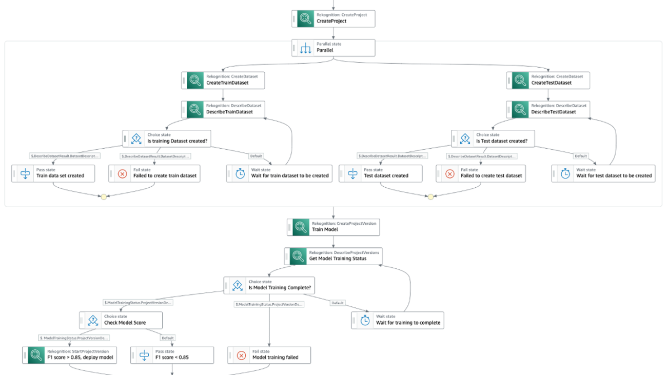
The following diagram illustrates the Step Functions workflow.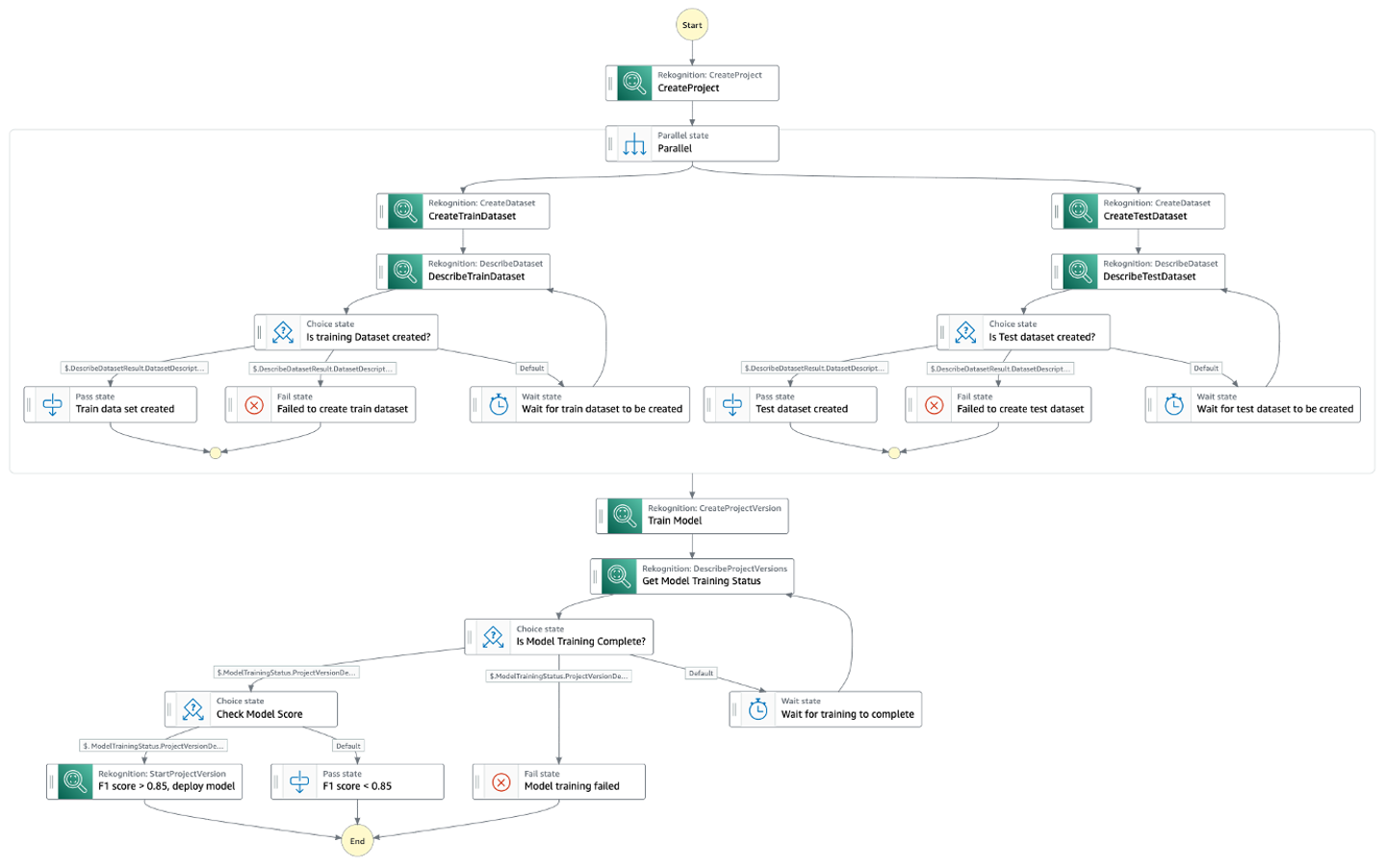
Prerequisites
Before deploying the workflow, we need to create the existing training and validation datasets. Complete the following steps:
- First, create an Amazon Rekognition project.
- Then, create the training and validation datasets.
- Finally, install the AWS SAM CLI.
Deploy the workflow
To deploy the workflow, clone the GitHub repository:
These commands build, package and deploy your application to AWS, with a series of prompts as explained in the repository.
Run the workflow
To test the workflow, navigate to the deployed workflow on the Step Functions console, then choose Start execution.
The workflow could take a few minutes to a few hours to complete. If the model passes the evaluation criteria, an endpoint for the model is created in Amazon Rekognition. If the model doesn’t pass the evaluation criteria or the training failed, the workflow fails. You can check the status of the workflow on the Step Functions console. For more information, refer to Viewing and debugging executions on the Step Functions console.
Perform model predictions
To perform predictions against the model, you can call the Amazon Rekognition DetectCustomLabels API. To invoke this API, the caller needs to have the necessary AWS Identity and Access Management (IAM) permissions. For more details on performing predictions using this API, refer to Analyzing an image with a trained model.
However, if you need to expose the DetectCustomLabels API publicly, you can front the DetectCustomLabels API with Amazon API Gateway. API Gateway is a fully managed service that makes it easy for developers to create, publish, maintain, monitor, and secure APIs at any scale. API Gateway acts as the front door for your DetectCustomLabels API, as shown in the following architecture diagram.
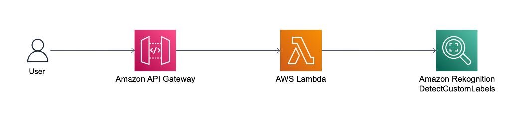
API Gateway forwards the user’s inference request to AWS Lambda. Lambda is a serverless, event-driven compute service that lets you run code for virtually any type of application or backend service without provisioning or managing servers. Lambda receives the API request and calls the Amazon Rekognition DetectCustomLabels API with the necessary IAM permissions. For more information on how to set up API Gateway with Lambda integration, refer to Set up Lambda proxy integrations in API Gateway.
The following is an example Lambda function code to call the DetectCustomLabels API:
Clean up
To delete the workflow, use the AWS SAM CLI:
To delete the Rekognition Custom Labels model, you can either use the Amazon Rekognition console or the AWS SDK. For more information, refer to Deleting an Amazon Rekognition Custom Labels model.
Conclusion
In this post, we walked through a Step Functions workflow to create a dataset and then train, evaluate, and use a Rekognition Custom Labels model. The workflow allows application developers and ML engineers to automate the custom label classification steps for any computer vision use case. The code for the workflow is open-sourced.
For more serverless learning resources, visit Serverless Land. To learn more about Rekognition custom labels, visit Amazon Rekognition Custom Labels.
About the Author
 Veda Raman is a Senior Specialist Solutions Architect for machine learning based in Maryland. Veda works with customers to help them architect efficient, secure and scalable machine learning applications. Veda is interested in helping customers leverage serverless technologies for Machine learning.
Build a machine learning model to predict student performance using Amazon SageMaker Canvas
There has been a paradigm change in the mindshare of education customers who are now willing to explore new technologies and analytics. Universities and other higher learning institutions have collected massive amounts of data over the years, and now they are exploring options to use that data for deeper insights and better educational outcomes.
You can use machine learning (ML) to generate these insights and build predictive models. Educators can also use ML to identify challenges in learning outcomes, increase success and retention among students, and broaden the reach and impact of online learning content.
However, higher education institutions often lack ML professionals and data scientists. With this fact, they are looking for solutions that can be quickly adopted by their existing business analysts.
Amazon SageMaker Canvas is a low-code/no-code ML service that enables business analysts to perform data preparation and transformation, build ML models, and deploy these models into a governed workflow. Analysts can perform all these activities with a few clicks and without writing a single piece of code.
In this post, we show how to use SageMaker Canvas to build an ML model to predict student performance.
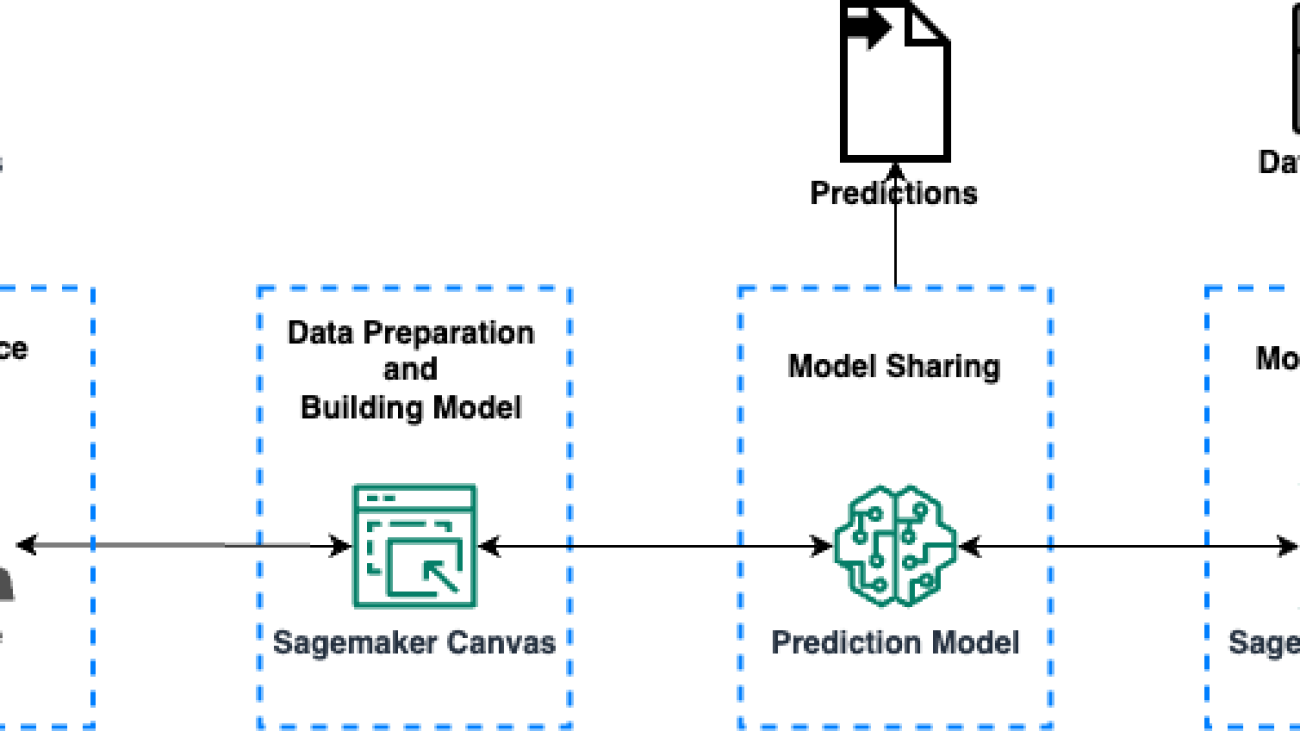
Solution overview
For this post, we discuss a specific use case: how universities can predict student dropout or continuation ahead of final exams using SageMaker Canvas. We predict whether the student will drop out, enroll (continue), or graduate at the end of the course. We can use the outcome from the prediction to take proactive action to improve student performance and prevent potential dropouts.
The solution includes the following components:
- Data ingestion – Importing the data from your local computer to SageMaker Canvas
- Data preparation – Clean and transform the data (if required) within SageMaker Canvas
- Build the ML model – Build the prediction model inside SageMaker Canvas to predict student performance
- Prediction – Generate batch or single predictions
- Collaboration – Analysts using SageMaker Canvas and data scientists using Amazon SageMaker Studio can interact while working in their respective settings, sharing domain knowledge and offering expert feedback to improve models
The following diagram illustrates the solution architecture.

Prerequisites
For this post, you should complete the following prerequisites:
- Have an AWS account.
- Set up SageMaker Canvas. For instructions, refer to Prerequisites for setting up Amazon SageMaker Canvas.
- Download the following student dataset to your local computer.
The dataset contains student background information like demographics, academic journey, economic background, and more. The dataset contains 37 columns, out of which 36 are features and 1 is a label. The label column name is Target, and it contains categorical data: dropout, enrolled, and graduate.
The dataset comes under the Attribution 4.0 International (CC BY 4.0) license and is free to share and adapt.
Data ingestion
The first step for any ML process is to ingest the data. Complete the following steps:
- On the SageMaker Canvas console, choose Import.
- Import the
Dropout_Academic Success - Sheet1.csvdataset into SageMaker Canvas. - Select the dataset and choose Create a model.
- Name the
model student-performance-model.

Data preparation
For ML problems, data scientists analyze the dataset for outliers, handle the missing values, add or remove fields, and perform other transformations. Analysts can perform the same actions in SageMaker Canvas using the visual interface. Note that major data transformation is out of scope for this post.
In the following screenshot, the first highlighted section (annotated as 1 in the screenshot) shows the options available with SageMaker Canvas. IT staff can apply these actions on the dataset and can even explore the dataset for more details by choosing Data visualizer.
The second highlighted section (annotated as 2 in the screenshot) indicates that the dataset doesn’t have any missing or mismatched records.

Build the ML model
To proceed with training and building the ML model, we need to choose the column that needs to be predicted.
- On the SageMaker Canvas interface, for Select a column to predict, choose Target.
As soon as you choose the target column, it will prompt you to validate data.
- Choose Validate, and within few minutes SageMaker Canvas will finish validating your data.
Now it’s the time to build the model. You have two options: Quick build and Standard build. Analysts can choose either of the options based on your requirements.
- For this post, we choose Standard build.

Apart from speed and accuracy, one major difference between Standard build and Quick build is that Standard build provides the capability to share the model with data scientists, which Quick build doesn’t.
SageMaker Canvas took approximately 25 minutes to train and build the model. Your models may take more or less time, depending on factors such as input data size and complexity. The accuracy of the model was around 80%, as shown in the following screenshot. You can explore the bottom section to see the impact of each column on the prediction.
So far, we have uploaded the dataset, prepared the dataset, and built the prediction model to measure student performance. Next, we have two options:
- Generate a batch or single prediction
- Share this model with the data scientists for feedback or improvements
Prediction
Choose Predict to start generating predictions. You can choose from two options:
- Batch prediction – You can upload datasets here and let SageMaker Canvas predict the performance for the students. You can use these predictions to take proactive actions.
- Single prediction – In this option, you provide the values for a single student. SageMaker Canvas will predict the performance for that particular student.

Collaboration
In some cases, you as an analyst might want to get feedback from expert data scientists on the model before proceeding with the prediction. To do so, choose Share and specify the Studio user to share with.

Then the data scientist can complete the following steps:
- On the Studio console, in the navigation pane, under Models, choose Shared models.
- Choose View model to open the model.

They can update the model either of the following ways:
- Share a new model – The data scientist can change the data transformations, retrain the model, and then share the model
- Share an alternate model – The data scientist can select an alternate model from the list of trained Amazon SageMaker Autopilot models and share that back with the SageMaker Canvas user.

For this example, we choose Share an alternate model and assume the inference latency as the key parameter shared the second-best model with the SageMaker Canvas user.
The data scientist can look for other parameters like F1 score, precision, recall, and log loss as decision criterion to share an alternate model with the SageMaker Canvas user.
In this scenario, the best model has an accuracy of 80% and inference latency of 0.781 seconds, whereas the second-best model has an accuracy of 79.9% and inference latency of 0.327 seconds.

- Choose Share to share an alternate model with the SageMaker Canvas user.
- Add the SageMaker Canvas user to share the model with.
- Add an optional note, then choose Share.
- Choose an alternate model to share.
- Add feedback and choose Share to share the model with the SageMaker Canvas user.

After the data scientist has shared an updated model with you, you will get a notification and SageMaker Canvas will start importing the model into the console.

SageMaker Canvas will take a moment to import the updated model, and then the updated model will reflect as a new version (V3 in this case).
You can now switch between the versions and generate predictions from any version.

If an administrator is worried about managing permissions for the analysts and data scientists, they can use Amazon SageMaker Role Manager.
Clean up
To avoid incurring future charges, delete the resources you created while following this post. SageMaker Canvas bills you for the duration of the session, and we recommend logging out of Canvas when you’re not using it. Refer to Logging out of Amazon SageMaker Canvas for more details.
Conclusion
In this post, we discussed how SageMaker Canvas can help higher learning institutions use ML capabilities without requiring ML expertise. In our example, we showed how an analyst can quickly build a highly accurate predictive ML model without writing any code. The university can now act on those insights by specifically targeting students at risk of dropping out of a course with individualized attention and resources, benefitting both parties.
We demonstrated the steps starting from loading the data into SageMaker Canvas, building the model in Canvas, and receiving the feedback from data scientists via Studio. The entire process was completed through web-based user interfaces.
To start your low-code/no-code ML journey, refer to Amazon SageMaker Canvas.
About the author
 Ashutosh Kumar is a Solutions Architect with the Public Sector-Education Team. He is passionate about transforming businesses with digital solutions. He has good experience in databases, AI/ML, data analytics, compute, and storage.
Access Snowflake data using OAuth-based authentication in Amazon SageMaker Data Wrangler
In this post, we show how to configure a new OAuth-based authentication feature for using Snowflake in Amazon SageMaker Data Wrangler. Snowflake is a cloud data platform that provides data solutions for data warehousing to data science. Snowflake is an AWS Partner with multiple AWS accreditations, including AWS competencies in machine learning (ML), retail, and data and analytics.
Data Wrangler simplifies the data preparation and feature engineering process, reducing the time it takes from weeks to minutes by providing a single visual interface for data scientists to select and clean data, create features, and automate data preparation in ML workflows without writing any code. You can import data from multiple data sources, such as Amazon Simple Storage Service (Amazon S3), Amazon Athena, Amazon Redshift, Amazon EMR, and Snowflake. With this new feature, you can use your own identity provider (IdP) such as Okta, Azure AD, or Ping Federate to connect to Snowflake via Data Wrangler.
Solution overview
In the following sections, we provide steps for an administrator to set up the IdP, Snowflake, and Studio. We also detail the steps that data scientists can take to configure the data flow, analyze the data quality, and add data transformations. Finally, we show how to export the data flow and train a model using SageMaker Autopilot.
Prerequisites
For this walkthrough, you should have the following prerequisites:
- For admin:
- A Snowflake user with permissions to create storage integrations, and security integrations in Snowflake.
- An AWS account with permissions to create AWS Identity and Access Management (IAM) policies and roles.
- Access and permissions to configure IDP to register Data Wrangler application and set up the authorization server or API.
- For data scientist:
- An S3 bucket that Data Wrangler can use to output transformed data.
- Access to Amazon SageMaker, an instance of Amazon SageMaker Studio, and a user for Studio. For more information about prerequisites, see Get Started with Data Wrangler.
- An IAM role used for Studio with permissions to create and update secrets in AWS Secrets Manager.
Administrator setup
Instead of having your users directly enter their Snowflake credentials into Data Wrangler, you can have them use an IdP to access Snowflake.
The following steps are involved to enable Data Wrangler OAuth access to Snowflake:
- Configure the IdP.
- Configure Snowflake.
- Configure SageMaker Studio.
Configure the IdP
To set up your IdP, you must register the Data Wrangler application and set up your authorization server or API.
Register the Data Wrangler application within the IdP
Refer to the following documentation for the IdPs that Data Wrangler supports:
Use the documentation provided by your IdP to register your Data Wrangler application. The information and procedures in this section help you understand how to properly use the documentation provided by your IdP.
Specific customizations in addition to the steps in the respective guides are called out in the subsections.
- Select the configuration that starts the process of registering Data Wrangler as an application.
- Provide the users within the IdP access to Data Wrangler.
- Enable OAuth client authentication by storing the client credentials as a Secrets Manager secret.
- Specify a redirect URL using the following format:
https://domain-ID.studio.AWS Region.sagemaker.aws/jupyter/default/lab.
You’re specifying the SageMaker domain ID and AWS Region that you’re using to run Data Wrangler. You must register a URL for each domain and Region where you’re running Data Wrangler. Users from a domain and Region that don’t have redirect URLs set up for them won’t be able to authenticate with the IdP to access the Snowflake connection.
- Make sure the authorization code and refresh token grant types are allowed for your Data Wrangler application.
Set up the authorization server or API within the IdP
Within your IdP, you must set up an authorization server or an application programming interface (API). For each user, the authorization server or the API sends tokens to Data Wrangler with Snowflake as the audience.
Snowflake uses the concept of roles that are distinct from IAM roles used in AWS. You must configure the IdP to use ANY Role to use the default role associated with the Snowflake account. For example, if a user has systems administrator as the default role in their Snowflake profile, the connection from Data Wrangler to Snowflake uses systems administrator as the role.
Use the following procedure to set up the authorization server or API within your IdP:
- From your IdP, begin the process of setting up the server or API.
- Configure the authorization server to use the authorization code and refresh token grant types.
- Specify the lifetime of the access token.
- Set the refresh token idle timeout.
The idle timeout is the time that the refresh token expires if it’s not used. If you’re scheduling jobs in Data Wrangler, we recommend making the idle timeout time greater than the frequency of the processing job. Otherwise, some processing jobs might fail because the refresh token expired before they could run. When the refresh token expires, the user must re-authenticate by accessing the connection that they’ve made to Snowflake through Data Wrangler.
Note that Data Wrangler doesn’t support rotating refresh tokens. Using rotating refresh tokens might result in access failures or users needing to log in frequently.
If the refresh token expires, your users must reauthenticate by accessing the connection that they’ve made to Snowflake through Data Wrangler.
- Specify
session:role-anyas the new scope.
For Azure AD, you must also specify a unique identifier for the scope.
After you’ve set up the OAuth provider, you provide Data Wrangler with the information it needs to connect to the provider. You can use the documentation from your IdP to get values for the following fields:
- Token URL – The URL of the token that the IdP sends to Data Wrangler
- Authorization URL – The URL of the authorization server of the IdP
- Client ID – The ID of the IdP
- Client secret – The secret that only the authorization server or API recognizes
- OAuth scope – This is for Azure AD only
Configure Snowflake
To configure Snowflake, complete the instructions in Import data from Snowflake.
Use the Snowflake documentation for your IdP to set up an external OAuth integration in Snowflake. See the previous section Register the Data Wrangler application within the IdP for more information on how to set up an external OAuth integration.
When you’re setting up the security integration in Snowflake, make sure you activate external_oauth_any_role_mode.
Configure SageMaker Studio
You store the fields and values in a Secrets Manager secret and add it to the Studio Lifecycle Configuration that you’re using for Data Wrangler. A Lifecycle Configuration is a shell script that automatically loads the credentials stored in the secret when the user logs into Studio. For information about creating secrets, see Move hardcoded secrets to AWS Secrets Manager. For information about using Lifecycle Configurations in Studio, see Use Lifecycle Configurations with Amazon SageMaker Studio.
Create a secret for Snowflake credentials
To create your secret for Snowflake credentials, complete the following steps:
- On the Secrets Manager console, choose Store a new secret.
- For Secret type, select Other type of secret.
- Specify the details of your secret as key-value pairs.
Key names require lowercase letters due to case sensitivity. Data Wrangler gives a warning if you enter any of these incorrectly. Input the secret values as key-value pairs Key/value if you’d like, or use the Plaintext option.
The following is the format of the secret used for Okta. If you are using Azure AD, you need to add the datasource_oauth_scope field.
- Update the preceding values with your choice of IdP and information gathered after application registration.
- Choose Next.
- For Secret name, add the prefix
AmazonSageMaker(for example, our secret isAmazonSageMaker-DataWranglerSnowflakeCreds). - In the Tags section, add a tag with the key
SageMakerand valuetrue. - Choose Next.
- The rest of the fields are optional; choose Next until you have the option to choose Store to store the secret.
After you store the secret, you’re returned to the Secrets Manager console.
- Choose the secret you just created, then retrieve the secret ARN.
- Store this in your preferred text editor for use later when you create the Data Wrangler data source.
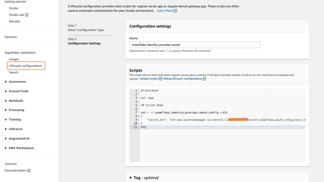
Create a Studio Lifecycle Configuration
To create a Lifecycle Configuration in Studio, complete the following steps:
- On the SageMaker console, choose Lifecycle configurations in the navigation pane.
- Choose Create configuration.
- Choose Jupyter server app.
- Create a new lifecycle configuration or append an existing one with the following content:
The configuration creates a file with the name ".snowflake_identity_provider_oauth_config", containing the secret in the user’s home folder.
- Choose Create Configuration.

Set the default Lifecycle Configuration
Complete the following steps to set the Lifecycle Configuration you just created as the default:
- On the SageMaker console, choose Domains in the navigation pane.
- Choose the Studio domain you’ll be using for this example.
- On the Environment tab, in the Lifecycle configurations for personal Studio apps section, choose Attach.

- For Source, select Existing configuration.
- Select the configuration you just made, then choose Attach to domain.

- Select the new configuration and choose Set as default, then choose Set as default again in the pop-up message.
Your new settings should now be visible under Lifecycle configurations for personal Studio apps as default.

- Shut down the Studio app and relaunch for the changes to take effect.
Data scientist experience
In this section, we cover how data scientists can connect to Snowflake as a data source in Data Wrangler and prepare data for ML.
Create a new data flow
To create your data flow, complete the following steps:
- On the SageMaker console, choose Amazon SageMaker Studio in the navigation pane.
- Choose Open Studio.
- On the Studio Home page, choose Import & prepare data visually. Alternatively, on the File drop-down, choose New, then choose SageMaker Data Wrangler Flow.
Creating a new flow can take a few minutes.

- On the Import data page, choose Create connection.
- Choose Snowflake from the list of data sources.

- For Authentication method, choose OAuth.
If you don’t see OAuth, verify the preceding Lifecycle Configuration steps.
- Enter details for Snowflake account name and Storage integration.
- Ener a connection name and choose Connect.

You’re redirected to an IdP authentication page. For this example, we’re using Okta.
- Enter your user name and password, then choose Sign in.

After the authentication is successful, you’re redirected to the Studio data flow page.
- On the Import data from Snowflake page, browse the database objects, or run a query for the targeted data.
- In the query editor, enter a query and preview the results.
In the following example, we load Loan Data and retrieve all columns from 5,000 rows.
- Choose Import.

- Enter a dataset name (for this post, we use
snowflake_loan_dataset) and choose Add.
You’re redirected to the Prepare page, where you can add transformations and analyses to the data.
Data Wrangler makes it easy to ingest data and perform data preparation tasks such as exploratory data analysis, feature selection, and feature engineering. We’ve only covered a few of the capabilities of Data Wrangler in this post on data preparation; you can use Data Wrangler for more advanced data analysis such as feature importance, target leakage, and model explainability using an easy and intuitive user interface.
Analyze data quality
Use the Data Quality and Insights Report to perform an analysis of the data that you’ve imported into Data Wrangler. Data Wrangler creates the report from the sampled data.
- On the Data Wrangler flow page, choose the plus sign next to Data types, then choose Get data insights.

- Choose Data Quality And Insights Report for Analysis type.
- For Target column, choose your target column.
- For Problem type, select Classification.
- Choose Create.

The insights report has a brief summary of the data, which includes general information such as missing values, invalid values, feature types, outlier counts, and more. You can either download the report or view it online.

Add transformations to the data
Data Wrangler has over 300 built-in transformations. In this section, we use some of these transformations to prepare the dataset for an ML model.
- On the Data Wrangler flow page, choose plus sign, then choose Add transform.
If you’re following the steps in the post, you’re directed here automatically after adding your dataset.

- Verify and modify the data type of the columns.
Looking through the columns, we identify that MNTHS_SINCE_LAST_DELINQ and MNTHS_SINCE_LAST_RECORD should most likely be represented as a number type rather than string.

- After applying the changes and adding the step, you can verify the column data type is changed to float.

Looking through the data, we can see that the fields EMP_TITLE, URL, DESCRIPTION, and TITLE will likely not provide value to our model in our use case, so we can drop them.
- Choose Add Step, then choose Manage columns.
- For Transform, choose Drop column.
- For Column to drop, specify
EMP_TITLE,URL,DESCRIPTION, andTITLE. - Choose Preview and Add.

Next, we want to look for categorical data in our dataset. Data Wrangler has a built-in functionality to encode categorical data using both ordinal and one-hot encodings. Looking at our dataset, we can see that the TERM, HOME_OWNERSHIP, and PURPOSE columns all appear to be categorical in nature.
- Add another step and choose Encode categorical.
- For Transform, choose One-hot encode.
- For Input column, choose
TERM. - For Output style, choose Columns.
- Leave all other settings as default, then choose Preview and Add.

The HOME_OWNERSHIP column has four possible values: RENT, MORTGAGE, OWN, and other.
- Repeat the preceding steps to apply a one-hot encoding approach on these values.
Lastly, the PURPOSE column has several possible values. For this data, we use a one-hot encoding approach as well, but we set the output to a vector rather than columns.
- For Transform, choose One-hot encode.
- For Input column, choose
PURPOSE. - For Output style, choose Vector.
- For Output column, we call this column
PURPOSE_VCTR.
This keeps the original PURPOSE column, if we decide to use it later.
- Leave all other settings as default, then choose Preview and Add.

Export the data flow
Finally, we export this whole data flow to a feature store with a SageMaker Processing job, which creates a Jupyter notebook with the code pre-populated.
- On the data flow page , choose the plus sign and Export to.
- Choose where to export. For our use case, we choose SageMaker Feature Store.

The exported notebook is now ready to run.


Export data and train a model with Autopilot
Now we can train the model using Amazon SageMaker Autopilot.
- On the data flow page, choose the Training tab.
- For Amazon S3 location, enter a location for the data to be saved.
- Choose Export and train.

- Specify the settings in the Target and features, Training method, Deployment and advance settings, and Review and create sections.
- Choose Create experiment to find the best model for your problem.
Clean up
If your work with Data Wrangler is complete, shut down your Data Wrangler instance to avoid incurring additional fees.
Conclusion
In this post, we demonstrated connecting Data Wrangler to Snowflake using OAuth, transforming and analyzing a dataset, and finally exporting it to the data flow so that it could be used in a Jupyter notebook. Most notably, we created a pipeline for data preparation without having to write any code at all.
To get started with Data Wrangler, see Prepare ML Data with Amazon SageMaker Data Wrangler.
About the authors
 Ajjay Govindaram is a Senior Solutions Architect at AWS. He works with strategic customers who are using AI/ML to solve complex business problems. His experience lies in providing technical direction as well as design assistance for modest to large-scale AI/ML application deployments. His knowledge ranges from application architecture to big data, analytics, and machine learning. He enjoys listening to music while resting, experiencing the outdoors, and spending time with his loved ones.
 Bosco Albuquerque is a Sr. Partner Solutions Architect at AWS and has over 20 years of experience in working with database and analytics products from enterprise database vendors and cloud providers. He has helped large technology companies design data analytics solutions and has led engineering teams in designing and implementing data analytics platforms and data products.
 Matt Marzillo is a Sr. Partner Sales Engineer at Snowflake. He has 10 years of experience in data science and machine learning roles both in consulting and with industry organizations. Matt has experience developing and deploying AI and ML models across many different organizations in areas such as marketing, sales, operations, clinical, and finance, as well as advising in consultative roles.
 Huong Nguyen is a product leader for Amazon SageMaker Data Wrangler at AWS. She has 15 years of experience creating customer-obsessed and data-driven products for both enterprise and consumer spaces. In her spare time, she enjoys audio books, gardening, hiking, and spending time with her family and friends.
It Takes a Village: 100+ NVIDIA MLOps and AI Platform Partners Help Enterprises Move AI Into Production
Building AI applications is hard. Putting them to use across a business can be even harder.
Less than one-third of enterprises that have begun adopting AI actually have it in production, according to a recent IDC survey.
Businesses often realize the full complexity of operationalizing AI just prior to launching an application. Problems discovered so late can seem insurmountable, so the deployment effort is often stalled and forgotten.
To help enterprises get AI deployments across the finish line, more than 100 machine learning operations (MLOps) software providers are working with NVIDIA. These MLOps pioneers provide a broad array of solutions to support businesses in optimizing their AI workflows for both existing operational pipelines and ones built from scratch.
Many NVIDIA MLOps and AI platform ecosystem partners as well as DGX-Ready Software partners, including Canonical, ClearML, Dataiku, Domino Data Lab, Run:ai and Weights & Biases, are building solutions that integrate with NVIDIA-accelerated infrastructure and software to meet the needs of enterprises operationalizing AI.
NVIDIA cloud service provider partners Amazon Web Services, Google Cloud, Azure, Oracle Cloud as well as other partners around the globe, such as Alibaba Cloud, also provide MLOps solutions to streamline AI deployments.
NVIDIA’s leading MLOps software partners are verified and certified for use with the NVIDIA AI Enterprise software suite, which provides an end-to-end platform for creating and accelerating production AI. Paired with NVIDIA AI Enterprise, the tools from NVIDIA’s MLOps partners help businesses develop and deploy AI successfully.
Enterprises can get AI up and running with help from these and other NVIDIA MLOps and AI platform partners:
- Canonical: Aims to accelerate at-scale AI deployments while making open source accessible for AI development. Canonical announced that Charmed Kubeflow is now certified as part of the DGX-Ready Software program, both on single-node and multi-node deployments of NVIDIA DGX systems. Designed to automate machine learning workflows, Charmed Kubeflow creates a reliable application layer where models can be moved to production.
- ClearML: Delivers a unified, open-source platform for continuous machine learning — from experiment management and orchestration to increased performance and ML production — trusted by teams at 1,300 enterprises worldwide. With ClearML, enterprises can orchestrate and schedule jobs on personalized compute fabric. Whether on premises or in the cloud, businesses can enjoy enhanced visibility over infrastructure usage while reducing compute, hardware and resource spend to optimize cost and performance. Now certified to run NVIDIA AI Enterprise, ClearML’s MLOps platform is more efficient across workflows, enabling greater optimization for GPU power.
- Dataiku: As the platform for Everyday AI, Dataiku enables data and domain experts to work together to build AI into their daily operations. Dataiku is now certified as part of the NVIDIA DGX-Ready Software program, which allows enterprises to confidently use Dataiku’s MLOps capabilities along with NVIDIA DGX AI supercomputers.
- Domino Data Lab: Offers a single pane of glass that enables the world’s most sophisticated companies to run data science and machine learning workloads in any compute cluster — in any cloud or on premises in all regions. Domino Cloud, a new fully managed MLOps platform-as-a-service, is now available for fast and easy data science at scale. Certified to run on NVIDIA AI Enterprise last year, Domino Data Lab’s platform mitigates deployment risks and ensures reliable, high-performance integration with NVIDIA AI.
- Run:ai: Functions as a foundational layer within enterprises’ MLOps and AI Infrastructure stacks through its AI computing platform, Atlas. The platform’s automated resource management capabilities allow organizations to properly align resources across different MLOps platforms and tools running on top of Run:ai Atlas. Certified to offer NVIDIA AI Enterprise, Run:ai is also fully integrating NVIDIA Triton Inference Server, maximizing the utilization and value of GPUs in AI-powered environments.
- Weights & Biases (W&B): Helps machine learning teams build better models, faster. With just a few lines of code, practitioners can instantly debug, compare and reproduce their models — all while collaborating with their teammates. W&B is trusted by more than 500,000 machine learning practitioners from leading companies and research organizations around the world. Now validated to offer NVIDIA AI Enterprise, W&B looks to accelerate deep learning workloads across computer vision, natural language processing and generative AI.
NVIDIA cloud service provider partners have integrated MLOps into their platforms that provide NVIDIA accelerated computing and software for data processing, wrangling, training and inference:
- Amazon Web Services: Amazon SageMaker for MLOps helps developers automate and standardize processes throughout the machine learning lifecycle, using NVIDIA accelerated computing. This increases productivity by training, testing, troubleshooting, deploying and governing ML models.
- Google Cloud: Vertex AI is a fully managed ML platform that helps fast-track ML deployments by bringing together a broad set of purpose-built capabilities. Vertex AI’s end-to-end MLOps capabilities make it easier to train, orchestrate, deploy and manage ML at scale, using NVIDIA GPUs optimized for a wide variety of AI workloads. Vertex AI also supports leading-edge solutions such as the NVIDIA Merlin framework, which maximizes performance and simplifies model deployment at scale. Google Cloud and NVIDIA collaborated to add Triton Inference Server as a backend on Vertex AI Prediction, Google Cloud’s fully managed model-serving platform.
- Azure: The Azure Machine Learning cloud platform is accelerated by NVIDIA and unifies ML model development and operations (DevOps). It applies DevOps principles and practices — like continuous integration, delivery and deployment — to the machine learning process, with the goal of speeding experimentation, development and deployment of Azure machine learning models into production. It provides quality assurance through built-in responsible AI tools to help ML professionals develop fair, explainable and responsible models.
- Oracle Cloud: Oracle Cloud Infrastructure (OCI) AI Services is a collection of services with prebuilt machine learning models that make it easier for developers to apply NVIDIA-accelerated AI to applications and business operations. Teams within an organization can reuse the models, datasets and data labels across services. OCI AI Services makes it possible for developers to easily add machine learning to apps without slowing down application development.
- Alibaba Cloud: Alibaba Cloud Machine Learning Platform for AI provides an all-in-one machine learning service featuring low user technical skills requirements, but with high performance results. Accelerated by NVIDIA, the Alibaba Cloud platform enables enterprises to quickly establish and deploy machine learning experiments to achieve business objectives.
Learn more about NVIDIA MLOps partners and their work at NVIDIA GTC, a global conference for the era of AI and the metaverse, running online through Thursday, March 23.
Watch NVIDIA founder and CEO Jensen Huang’s GTC keynote in replay:

PyTorch 2.0 & XLA—The Latest Cutting Edge Features
Today, we are excited to share our latest work for PyTorch/XLA 2.0. The release of PyTorch 2.0 is yet another major milestone for this storied community and we are excited to continue to be part of it. When the PyTorch/XLA project started in 2018 between Google and Meta, the focus was on bringing cutting edge Cloud TPUs to help support the PyTorch community. Along the way, others in the community such as Amazon joined the project and very quickly the community expanded. We are excited about XLA’s direction and the benefits this project continues to bring to the PyTorch community. In this blog we’d like to showcase some key features that have been in development, show code snippets, and illustrate the benefit through some benchmarks.
TorchDynamo / torch.compile (Experimental)
TorchDynamo (Dynamo) is a Python-level JIT compiler designed to make unmodified PyTorch programs faster. It provides a clean API for compiler backends to hook in; its biggest feature is to dynamically modify Python bytecode just before execution. In the PyTorch/XLA 2.0 release, an experimental backend for Dynamo is provided for both inference and training.
Dynamo provides a Torch FX (FX) graph when it recognizes a model pattern and PyTorch/XLA uses a Lazy Tensor approach to compile the FX graph and return the compiled function. To get more insight regarding the technical details about PyTorch/XLA’s dynamo implementation, check out this dev-discuss post and dynamo doc.
Here is a small code example of running ResNet18 with torch.compile:
import torch
import torchvision
import torch_xla.core.xla_model as xm

def eval_model(loader):
  device = xm.xla_device()
  xla_resnet18 = torchvision.models.resnet18().to(device)
  xla_resnet18.eval()
  dynamo_resnet18 = torch.compile(
      xla_resnet18, backend='torchxla_trace_once')
  for data, _ in loader:
    output = dynamo_resnet18(data)
With torch.compile PyTorch/XLA only traces the ResNet18 model once during the init time and executes the compiled binary everytime dynamo_resnet18 is invoked, instead of tracing the model every step. To illustrate the benefits of Dynamo+XLA, below is an inference speedup analysis to compare Dynamo and LazyTensor (without Dynamo) using TorchBench on a Cloud TPU v4-8 where the y-axis is the speedup multiplier.
Dynamo for training is in the development stage with its implementation being at an earlier stage than inference. Developers are welcome to test this early feature, however, in the 2.0 release, PyTorch/XLA supports the forward and backward pass graphs and not the optimizer graph; the optimizer graph is available in the nightly builds and will land in the PyTorch/XLA 2.1 release. Below is an example of what training looks like using the ResNet18 example with torch.compile:
import torch
import torchvision
import torch_xla.core.xla_model as xm

def train_model(model, data, target):
  loss_fn = torch.nn.CrossEntropyLoss()
  pred = model(data)
  loss = loss_fn(pred, target)
  loss.backward()
  return pred

def train_model_main(loader):
  device = xm.xla_device()
  xla_resnet18 = torchvision.models.resnet18().to(device)
  xla_resnet18.train()
  dynamo_train_model = torch.compile(
        train_model, backend='aot_torchxla_trace_once')
  for data, target in loader:
    output = dynamo_train_model(xla_resnet18, data, target)
Note that the backend for training is aot_torchxla_trace_once (API will be updated for stable release) whereas the inference backend is torchxla_trace_once (name subject to change). We expect to extract and execute 3 graphs per training step instead of 1 training step if you use the Lazy tensor. Below is a training speedup analysis to compare Dynamo and Lazy using the TorchBench on Cloud TPU v4-8.

PJRT Runtime (Beta)
PyTorch/XLA is migrating from XRT to the new PJRT runtime. PJRT is a better-maintained stack, with demonstrated performance advantages, including, on average, a 35% performance for training on TorchBench 2.0 models. It also supports a richer set of features enabling technologies like SPMD. In the PyTorch/XLA 2.0 release, PJRT is the default runtime for TPU and CPU; GPU support is in experimental state. The PJRT features included in the PyTorch/XLA 2.0 release are:
- TPU runtime implementation in
libtpuusing the PJRT Plugin API improves performance by up to 30% torch.distributedsupport for TPU v2 and v3, includingpjrt://init_method(Experimental)- Single-host GPU support. Multi-host support coming soon. (Experimental)
Switching to PJRT requires no change (or minimal change for GPUs) to user code (see pjrt.md for more details). Runtime configuration is as simple as setting the PJRT_DEVICE environment variable to the local device type (i.e. TPU, GPU, CPU). Below are examples of using PJRT runtimes on different devices.
# TPU Device
PJRT_DEVICE=TPU python3 xla/test/test_train_mp_imagenet.py --fake_data --batch_size=256 --num_epochs=1
# TPU Pod Device
gcloud alpha compute tpus tpu-vm ssh $USER-pjrt --zone=us-central2-b --project=$PROJECT --worker=all --command="git clone --depth=1 --branch r2.0 https://github.com/pytorch/xla.git"

gcloud alpha compute tpus tpu-vm ssh $USER-pjrt --zone=us-central2-b --project=$PROJECT --worker=all --command="PJRT_DEVICE=TPU python3 xla/test/test_train_mp_imagenet.py --fake_data --batch_size=256 --num_epochs=1"
# GPU Device (Experimental)
PJRT_DEVICE=GPU GPU_NUM_DEVICES=4 python3 xla/test/test_train_mp_imagenet.py --fake_data --batch_size=128 --num_epochs=1
Below is a performance comparison between XRT and PJRT by task on TorchBench 2.0 on v4-8 TPU. To learn more about PJRT vs. XRT please review the documentation.

Parallelization
GSPMD (Experimental)
We are delighted to introduce General and Scalable Parallelization for ML Computation Graphs (GSPMD) in PyTorch as a new experimental data & model sharding solution. GSPMD provides automatic parallelization for common ML workloads, allowing developers to write PyTorch programs as if on a single large device and without custom sharded computation ops and/or collective communication ops. The XLA compiler transforms the single device program into a partitioned one with proper collectives, based on the user provided sharding hints. The API (RFC) will be available in the PyTorch/XLA 2.0 release as an experimental feature on a single TPU VM host.
Next Steps for GSPMD
GSPMD is experimental in 2.0 release. To bring it to Stable status, we plan to address a number of feature gaps and known issues in the following releases, including multi-host support, DTensor integration, partial replication sharding, asynchronous data loading, and checkpointing.
FSDP (Beta)
PyTorch/XLA introduced fully sharded data parallel (FSDP) experimental support in version 1.12. This feature is a parallel representation of PyTorch FSDP and there are subtle differences in how XLA and upstream CUDA kernels are set up. auto_wrap_policy is a new argument that enables developers to automatically specify conditions for propagating partitioning specifications to neural network submodules. auto_wrap_policys may be simply passed in as an argument when wrapping a model with FSDP. Two auto_wrap_policy callables worth noting are: size_based_auto_wrap_policy, transformer_auto_wrap_policy.
size_based_auto_wrap_policy enables users to wrap submodules with a minimum number of parameters. The example below wraps model submodules having at least 10M parameters.
auto_wrap_policy = partial(size_based_auto_wrap_policy, min_num_params=1e7)
transformer_auto_wrap_policy enables users to wrap all submodules that match a specific layer type. The example below wraps model submodules named torch.nn.Conv2d. To learn more, review this ResNet example by Ronghang Hu.
auto_wrap_policy = partial(transformer_auto_wrap_policy, transformer_layer_cls={torch.nn.Conv2d})
PyTorch/XLA FSDP is now integrated in HuggingFace trainer class (PR) enabling users to train much larger models on PyTorch/XLA (official Hugging Face documentation). A 16B parameters GPT2 model trained on Cloud TPU v4-64 with this FSDP configuration achieved 39% hardware utilization.
| TPU Accelerator – Num Devices | v4-64 |
| GPT2 Parameter Count | 16B |
| Layers Wrapped with FSDP | GPT2Block |
| TFLOPs / Chip | 275 |
| PFLOPs / Step | 50 |
| Hardware Utilization | 39% |
Differences Between FSDP & GSPMD
FSDP is a data parallelism technique that reduces device memory footprint by storing model parameters, optimizer states, and gradients all sharded. Note that the actual computation is still local to the device and requires all-gathering the sharded model parameters for both forward and backward passes, hence the name “data parallel”. FSDP is one of the newest additions to PyTorch/XLA to scale large model training.
GSPMD on the other hand, is a general parallelization system that enables various types of parallelisms, including both data and model parallelisms. PyTorch/XLA provides a sharding annotation API and XLAShardedTensor abstraction, so a user can annotate any tensor with sharding specs in the PyTorch program. Developers don’t need to manually implement sharded computations or inject collective communications ops to get it right. The XLA compiler does the work so that each computation can run in a distributed manner on multiple devices.
Examples & Preliminary Results
To learn about PyTorch/XLA parallelism sharding API, visit our RFC and see the Sample Code references. Below is a simple example to enable data and model parallelism.
model = SimpleLinear().to(xm.xla_device())
# Sharding annotate the linear layer weights.
xs.mark_sharding(model.fc1.weight, mesh, partition_spec)
# Training loop
model.train()
for step, (data, target) in enumerate(loader):
  optimizer.zero_grad()
  data = data.to(xm.xla_device())
  target = target.to(xm.xla_device())
  # Sharding annotate input data, we can shard any input
  # dimensions. Sharidng the batch dimension enables
  # data parallelism, sharding the feature dimension enables
  # spatial partitioning.
  xs.mark_sharding(data, mesh, partition_spec)
  ouput = model(data)
  loss = loss_fn(output, target)
  optimizer.step()
  xm.mark_step()
The following graph highlights the memory efficiency benefits of PyTorch/XLA FSDP and SPMD on Cloud TPU v4-8 running ResNet50.

Closing Thoughts…
We are excited to bring these features to the PyTorch community, and this is really just the beginning. Areas like dynamic shapes, deeper support for OpenXLA and many others are in development and we plan to put out more blogs to dive into the details. PyTorch/XLA is developed fully open source and we invite you to join the community of developers by filing issues, submitting pull requests, and sending RFCs on GitHub. You can try PyTorch/XLA on a variety of XLA devices including TPUs and GPUs. Here is how to get started.
Congratulations again to the PyTorch community on this milestone!
Cheers,
The PyTorch Team at Google
Remote monitoring of raw material supply chains for sustainability with Amazon SageMaker geospatial capabilities
Deforestation is a major concern in many tropical geographies where local rainforests are at severe risk of destruction. About 17% of the Amazon rainforest has been destroyed over the past 50 years, and some tropical ecosystems are approaching a tipping point beyond which recovery is unlikely.
A key driver for deforestation is raw material extraction and production, for example the production of food and timber or mining operations. Businesses consuming these resources are increasingly recognizing their share of responsibility in tackling the deforestation issue. One way they can do this is by ensuring that their raw material supply is produced and sourced sustainably. For example, if a business uses palm oil in their products, they will want to ensure that natural forests were not burned down and cleared to make way for a new palm oil plantation.
Geospatial analysis of satellite imagery taken of the locations where suppliers operate can be a powerful tool to detect problematic deforestation events. However, running such analyses is difficult, time-consuming, and resource-intensive. Amazon SageMaker geospatial capabilities—now generally available in the AWS Oregon Region—provide a new and much simpler solution to this problem. The tool makes it easy to access geospatial data sources, run purpose-built processing operations, apply pre-trained ML models, and use built-in visualization tools faster and at scale.
In this post, you will learn how to use SageMaker geospatial capabilities to easily baseline and monitor the vegetation type and density of areas where suppliers operate. Supply chain and sustainability professionals can use this solution to track the temporal and spatial dynamics of unsustainable deforestation in their supply chains. Specifically, the guidance provides data-driven insights into the following questions:
- When and over what period did deforestation occur – The guidance allows you to pinpoint when a new deforestation event occurred and monitor its duration, progression, or recovery
- Which type of land cover was most affected – The guidance allows you to pinpoint which vegetation types were most affected by a land cover change event (for example, tropical forests or shrubs)
- Where specifically did deforestation occur – Pixel-by-pixel comparisons between baseline and current satellite imagery (before vs. after) allow you to identify the precise locations where deforestation has occurred
- How much forest was cleared – An estimate on the affected area (in km2) is provided by taking advantage of the fine-grained resolution of satellite data (for example, 10mx10m raster cells for Sentinel 2)
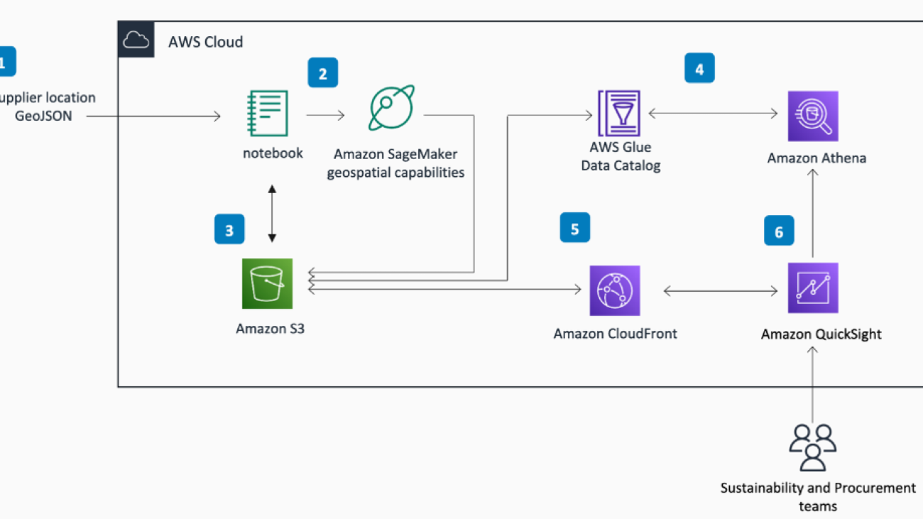
Solution overview
The solution uses SageMaker geospatial capabilities to retrieve up-to-date satellite imagery for any area of interest with just a few lines of code, and apply pre-built algorithms such as land use classifiers and band math operations. You can then visualize results using built-in mapping and raster image visualization tooling. To derive further insights from the satellite data, the guidance uses the export functionality of Amazon SageMaker to save the processed satellite imagery to Amazon Simple Storage Service (Amazon S3), where data is cataloged and shared for custom postprocessing and analysis in an Amazon SageMaker Studio notebook with a SageMaker geospatial image. Results of these custom analyses are subsequently published and made observable in Amazon QuickSight so that procurement and sustainability teams can review supplier location vegetation data in one place. The following diagram illustrates this architecture.

The notebooks and code with a deployment-ready implementation of the analyses shown in this post are available at the GitHub repository Guidance for Geospatial Insights for Sustainability on AWS.
Example use case
This post uses an area of interest (AOI) from Brazil where land clearing for cattle production, oilseed growing (soybean and palm oil), and timber harvesting is a major concern. You can also generalize this solution to any other desired AOI.
The following screenshot displays the AOI showing satellite imagery (visible band) from the European Space Agency’s Sentinel 2 satellite constellation retrieved and visualized in a SageMaker notebook. Agricultural regions are clearly visible against dark green natural rainforest. Note also the smoke originating from inside the AOI as well as a larger area to the North. Smoke is often an indicator of the use of fire in land clearing.

NDVI as a measure for vegetation density
To identify and quantify changes in forest cover over time, this solution uses the Normalized Difference Vegetation Index (NDVI). . NDVI is calculated from the visible and near-infrared light reflected by vegetation. Healthy vegetation absorbs most of the visible light that hits it, and reflects a large portion of the near-infrared light. Unhealthy or sparse vegetation reflects more visible light and less near-infrared light. The index is computed by combining the red (visible) and near-infrared (NIR) bands of a satellite image into a single index ranging from -1 to 1.
Negative values of NDVI (values approaching -1) correspond to water. Values close to zero (-0.1 to 0.1) represent barren areas of rock, sand, or snow. Lastly, low and positive values represent shrub, grassland, or farmland (approximately 0.2 to 0.4), whereas high NDVI values indicate temperate and tropical rainforests (values approaching 1). Learn more about NDVI calculations here). NDVI values can therefore be mapped easily to a corresponding vegetation class:
By tracking changes in NDVI over time using the SageMaker built-in NDVI model, we can infer key information on whether suppliers operating in the AOI are doing so responsibly or whether they’re engaging in unsustainable forest clearing activity.
Retrieve, process, and visualize NDVI data using SageMaker geospatial capabilities
One primary function of the SageMaker Geospatial API is the Earth Observation Job (EOJ), which allows you to acquire and transform raster data collected from the Earth’s surface. An EOJ retrieves satellite imagery from a specified data source (i.e., a satellite constellation) for a specified area of interest and time period, and applies one or several models to the retrieved images.
EOJs can be created via a geospatial notebook. For this post, we use an example notebook.
To configure an EOJ, set the following parameters:
- InputConfig – The input configuration defines data sources and filtering criteria to be applied during data acquisition:
- RasterDataCollectionArn – Defines which satellite to collect data from.
- AreaOfInterest – The geographical AOI; defines Polygon for which images are to be collected (in
GeoJSONformat). - TimeRangeFilter – The time range of interest:
{StartTime: <string>, EndTime: <string> }. - PropertyFilters – Additional property filters, such as maximum acceptable cloud cover.
- JobConfig – The model configuration defines the processing job to be applied to the retrieved satellite image data. An NDVI model is available as part of the pre-built
BandMathoperation.
Set InputConfig
SageMaker geospatial capabilities support satellite imagery from two different sources that can be referenced via their Amazon Resource Names (ARNs):
- Landsat Collection 2 Level-2 Science Products, which measures the Earth’s surface reflectance (SR) and surface temperature (ST) at a spatial resolution of 30m
- Sentinel 2 L2A COGs, which provides large-swath continuous spectral measurements across 13 individual bands (blue, green, near-infrared, and so on) with resolution down to 10m.
You can retrieve these ARNs directly via the API by calling list_raster_data_collections().
This solution uses Sentinel 2 data. The Sentinel-2 mission is based on a constellation of two satellites. As a constellation, the same spot over the equator is revisited every 5 days, allowing for frequent and high-resolution observations. To specify Sentinel 2 as data source for the EOJ, simply reference the ARN:
Next, the AreaOfInterest (AOI) for the EOJ needs to be defined. To do so, you need to provide a GeoJSON of the bounding box that defines the area where a supplier operates. The following code snippet extracts the bounding box coordinates and defines the EOJ request input:
The time range is defined using the following request syntax:
Depending on the raster data collection selected, different additional property filters are supported. You can review the available options by calling get_raster_data_collection(Arn=data_collection_arn)["SupportedFilters"]. In the following example, a tight limit of 5% cloud cover is imposed to ensure a relatively unobstructed view on the AOI:
Review query results
Before you start the EOJ, make sure that the query parameters actually result in satellite images being returned as a response. In this example, the ApproximateResultCount is 3, which is sufficient. You may need to use a less restrictive PropertyFilter if no results are returned.
You can review thumbnails of the raw input images by indexing the query_results object. For example, the raw image thumbnail URL of the last item returned by the query can be accessed as follows: query_results['Items'][-1]["Assets"]["thumbnail"]["Href"] .
Set JobConfig
Now that we have set all required parameters needed to acquire the raw Sentinel 2 satellite data, the next step is to infer vegetation density measured in terms of NDVI. This would typically involve identifying the satellite tiles that intersect the AOI and downloading the satellite imagery for the time frame in scope from a data provider. You would then have to go through the process of overlaying, merging, and clipping the acquired files, computing the NDVI per each raster cell of the combined image by performing mathematical operations on the respective bands (such as red and near-infrared), and finally saving the results to a new single-band raster image. SageMaker geospatial capabilities provide an end-to-end implementation of this workflow, including a built-in NDVI model that can be run with a simple API call. All you need to do is specify the job configuration and set it to the predefined NDVI model:
Having defined all required inputs for SageMaker to acquire and transform the geospatial data of interest, you can now start the EOJ with a simple API call:
After the EOJ is complete, you can start exploring the results. SageMaker geospatial capabilities provide built-in visualization tooling powered by Foursquare Studio, which natively works from within a SageMaker notebook via the SageMaker geospatial Map SDK. The following code snippet initializes and renders a map and then adds several layers to it:
Once rendered, you can interact with the map by hiding or showing layers, zooming in and out, or modifying color schemes, among other options. The following screenshot shows the AOI bounding box layer superimposed on the output layer (the NDVI-transformed Sentinel 2 raster file). Bright yellow patches represent rainforest that is intact (NDVI=1), darker patches represent fields (0.5>NDVI>0), and dark-blue patches represent water (NDVI=-1).

By comparing current period values vs. a defined baseline period, changes and anomalies in NDVI can be identified and tracked over time.
Custom postprocessing and QuickSight visualization for additional insights
SageMaker geospatial capabilities come with a powerful pre-built analysis and mapping toolkit that delivers the functionality needed for many geospatial analysis tasks. In some cases, you may require additional flexibility and want to run customized post-analyses on the EOJ results. SageMaker geospatial capabilities facilitate this flexibility via an export function. Exporting EOJ outputs is again a simple API call:
Then you can download the output raster files for further local processing in a SageMaker geospatial notebook using common Python libraries for geospatial analysis such as GDAL, Fiona, GeoPandas, Shapely, and Rasterio, as well as SageMaker-specific libraries. With the analyses running in SageMaker, all AWS analytics tooling that natively integrate with SageMaker are also at your disposal. For example, the solution linked in the Guidance for Geospatial Insights for Sustainability on AWS GitHub repo uses Amazon S3 and Amazon Athena for querying the postprocessing results and making them observable in a QuickSight dashboard. All processing routines along with deployment code and instructions for the QuickSight dashboard are detailed in the GitHub repository.
The dashboard offers three core visualization components:
- A time series plot of NDVI values normalized against a baseline period, which enables you to track the temporal dynamics in vegetation density
- Full discrete distribution of NDVI values in the baseline period and the current period, providing transparency on which vegetation types have seen the largest change
- NDVI-transformed satellite imagery for the baseline period, current period, and pixel-by-pixel differences between both periods, which allows you to identify the affected regions inside the AOI
As shown in the following example, over the period of 5 years (2017-Q3 to 2022-Q3), the average NDVI of AOI decreased by 7.6% against the baseline period (Q3 2017), affecting a total area of 250.21 km2. This reduction was primarily driven by changes in high-NDVI areas (forest, rainforest), which can be seen when comparing the NDVI distributions of the current vs. the baseline period.

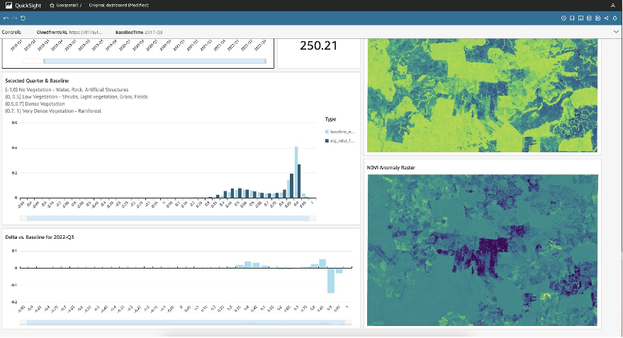
The pixel-by-pixel spatial comparison against the baseline highlights that the deforestation event occured in an area right at the center of the AOI where previously untouched natural forest has been converted into farmland. Supply chain professionals can take these data points as basis for further investigation and a potential review of relationships with the supplier in question.
Conclusion
SageMaker geospatial capabilities can form an integral part in tracking corporate climate action plans by making remote geospatial monitoring easy and accessible. This blog post focused on just one specific use case – monitoring raw material supply chain origins. Other use cases are easily conceivable. For example, you could use a similar architecture to track forest restoration efforts for emission offsetting, monitor plant health in reforestation or farming applications, or detect the impact of droughts on water bodies, among many other applications.
About the Authors
 Karsten Schroer is a Solutions Architect at AWS. He supports customers in leveraging data and technology to drive sustainability of their IT infrastructure and build cloud-native data-driven solutions that enable sustainable operations in their respective verticals. Karsten joined AWS following his PhD studies in applied machine learning & operations management. He is truly passionate about technology-enabled solutions to societal challenges and loves to dive deep into the methods and application architectures that underlie these solutions.
 Tamara Herbert is an Application Developer with AWS Professional Services in the UK. She specializes in building modern & scalable applications for a wide variety of customers, currently focusing on those within the public sector. She is actively involved in building solutions and driving conversations that enable organizations to meet their sustainability goals both in and through the cloud.
 Margaret O’Toole joined AWS in 2017 and has spent her time helping customers in various technical roles. Today, Margaret is the WW Tech Leader for Sustainability and leads a community of customer facing sustainability technical specialists. Together, the group helps customers optimize IT for sustainability and leverage AWS technology to solve some of the most difficult challenges in sustainability around the world. Margaret studied biology and computer science at the University of Virginia and Leading Sustainable Corporations at Oxford’s Saïd Business School.