Enable predictive maintenance for line of business users with Amazon Lookout for Equipment

Enable predictive maintenance for line of business users with Amazon Lookout for Equipment

Predictive maintenance is a data-driven maintenance strategy for monitoring industrial assets in order to detect anomalies in equipment operations and health that could lead to equipment failures. Through proactive monitoring of an asset’s condition, maintenance personnel can be alerted before issues occur, thereby avoiding costly unplanned downtime, which in turn leads to an increase in Overall Equipment Effectiveness (OEE).

However, building the necessary machine learning (ML) models for predictive maintenance is complex and time consuming. It requires several steps, including preprocessing of the data, building, training, evaluating, and then fine-tuning multiple ML models that can reliably predict anomalies in your asset’s data. The finished ML models then need to be deployed and provided with live data for online predictions (inferencing). Scaling this process to multiple assets of various types and operating profiles is often too resource intensive to make broader adoption of predictive maintenance viable.

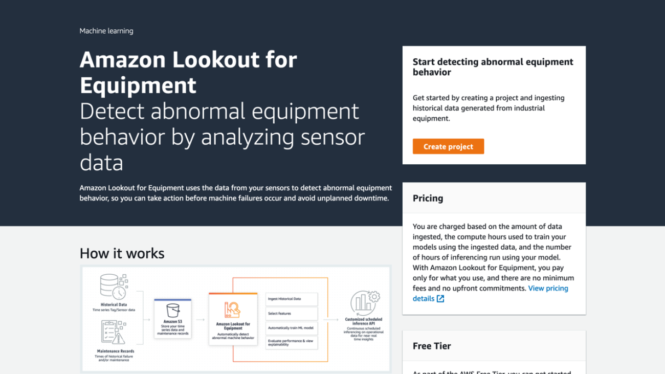
With Amazon Lookout for Equipment, you can seamlessly analyze sensor data for your industrial equipment to detect abnormal machine behavior—with no ML experience required.

When customers implement predictive maintenance use cases with Lookout for Equipment, they typically choose between three options to deliver the project: build it themselves, work with an AWS Partner, or use AWS Professional Services. Before committing to such projects, decision-makers such as plant managers, reliability or maintenance managers, and line leaders want to see evidence of the potential value that predictive maintenance can uncover in their lines of business. Such an evaluation is usually performed as part of a proof of concept (POC) and is the basis for a business case.

This post is directed to both technical and non-technical users: it provides an effective approach for evaluating Lookout for Equipment with your own data, allowing you to gauge the business value it provides your predictive maintenance activities.

Solution overview

In this post, we guide you through the steps to ingest a dataset in Lookout for Equipment, review the quality of the sensor data, train a model, and evaluate the model. Completing these steps will help derive insights into the health of your equipment.

Prerequisites

All you need to get started is an AWS account and a history of sensor data for assets that can benefit from a predictive maintenance approach. The sensor data should be stored as CSV files in an Amazon Simple Storage Service (Amazon S3) bucket from your account. Your IT team should be able to meet these prerequisites by referring to Formatting your data. To keep things simple, it’s best to store all the sensor data in one CSV file where the rows are timestamps and the columns are individual sensors (up to 300).

Once you have your dataset available on Amazon S3, you can follow along with the rest of this post.

Add a dataset

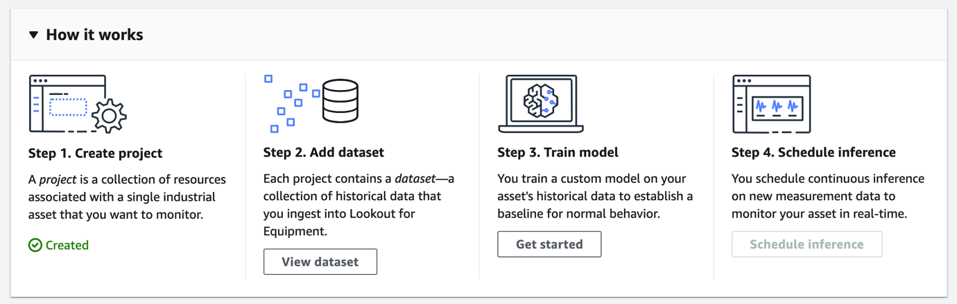
Lookout for Equipment uses projects to organize the resources for evaluating pieces of industrial equipment. To create a new project, complete the following steps:

  1. On the Lookout for Equipment console, choose Create project.

Click the Create Project button on the home page of the service

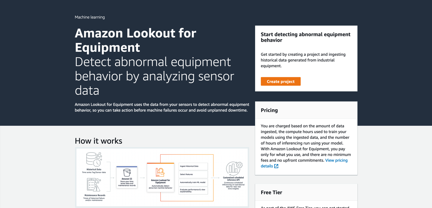
  1. Enter a project name and choose Create project.

After the project is created, you can ingest a dataset that will be used to train and evaluate a model for anomaly detection.

  1. On the project page, choose Add dataset.

Click Add dataset on the project dashboard

  1. For S3 location, enter the S3 location (excluding the file name) of your data.
  2. For Schema detection method, select By filename, which assumes that all sensor data for an asset is contained in a single CSV file at the specified S3 location.
  3. Keep the other settings as default and choose Start ingestion to start the ingestion process.

Configure your data source details and click Start ingestion

Ingestion may take around 10–20 minutes to complete. In the background, Lookout for Equipment performs the following tasks:

  • It detects the structure of the data, such as sensor names and data types.
  • The timestamps between sensors are aligned and missing values are filled (using the latest known value).
  • Duplicate timestamps are removed (only the last value for each timestamp is kept).
  • Lookout for Equipment uses multiple types of algorithms for building the ML anomaly detection model. During the ingestion phase, it prepares the data so it can be used for training those different algorithms.
  • It analyzes the measurement values and grades each sensor as high, medium, or low quality.
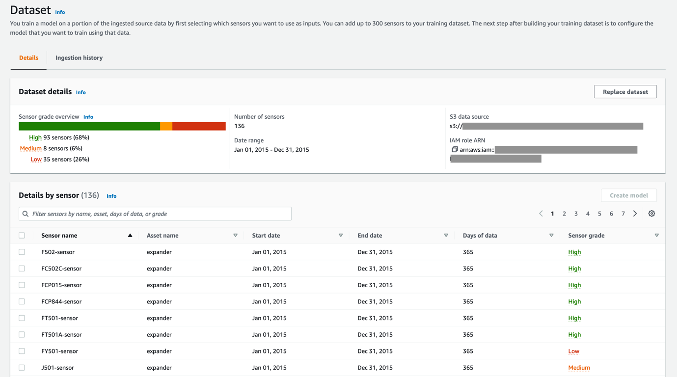
  1. When the dataset ingestion is complete, inspect it by choosing View dataset under Step 2 of the project page.

Click View dataset on the project dashboard

When creating an anomaly detection model, selecting the best sensors (the ones containing the highest data quality) is often critical to training models that deliver actionable insights. The Dataset details section shows the distribution of sensor gradings (between high, medium, and low), while the table displays information on each sensor separately (including the sensor name, date range, and grading for the sensor data). With this detailed report, you can make an informed decision about which sensors you will use to train your models. If a large proportion of sensors in your dataset are graded as medium or low, there might be a data issue needing investigation. If necessary, you can reupload the data file to Amazon S3 and ingest the data again by choosing Replace dataset.

Sensor grade dashboard overview

By choosing the sensor grade entry in the details table, you can review details on the validation errors resulting in a given grade. Displaying and addressing these details will help ensure information provided to the model is high quality. For example, you might see a signal has unexpected big chunks of missing values. Is this a data transfer issue, or was the sensor malfunctioning? Time to dive deeper in your data!

Individual sensor grade overview

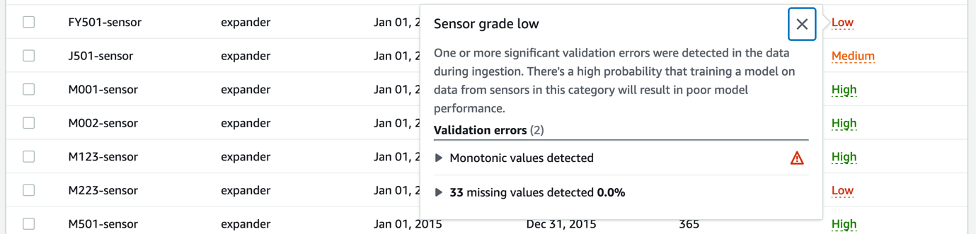
To learn more about the different type of sensor issues Lookout for Equipment addresses when grading your sensors, refer to Evaluating sensor grades. Developers can also extract these insights using the ListSensorStatistics API.

When you’re happy with your dataset, you can move to the next step of training a model for predicting anomalies.

Train a model

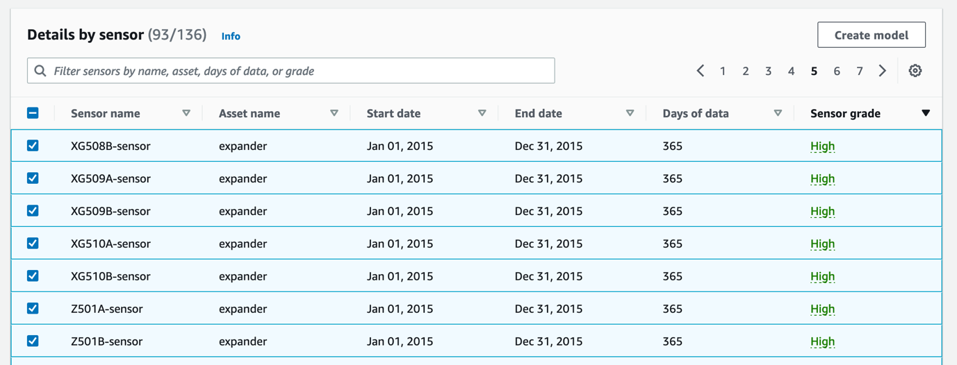
Lookout for Equipment allows the training of models for specific sensors. This gives you the flexibility to experiment with different sensor combinations or exclude sensors with a low grading. Complete the following steps:

  1. In the Details by sensor section on the dataset page, select the sensors to include in your model and choose Create model.

Selecting sensors for training a model

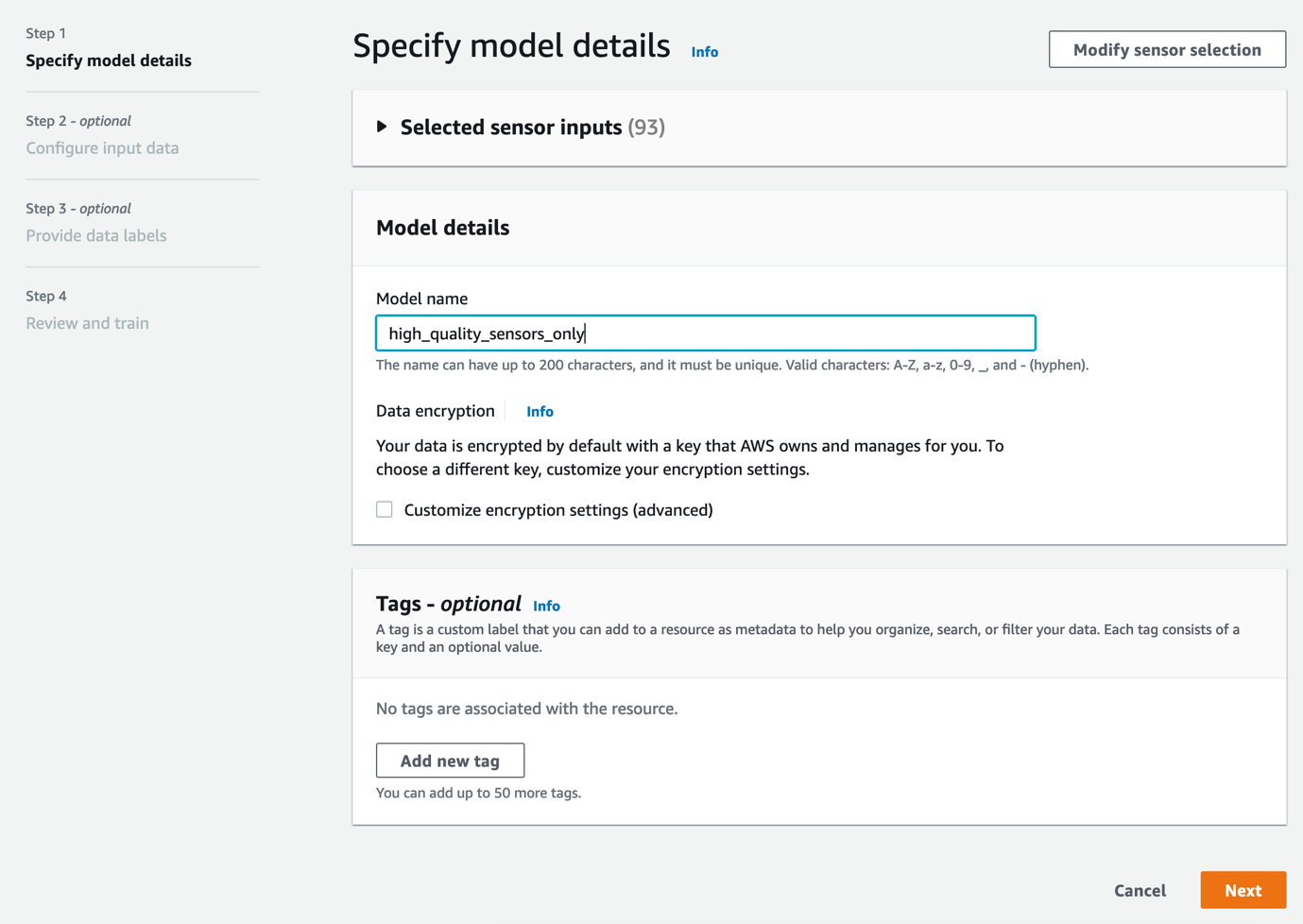
  1. For Model name, enter a model name, then choose Next.

Give a model name

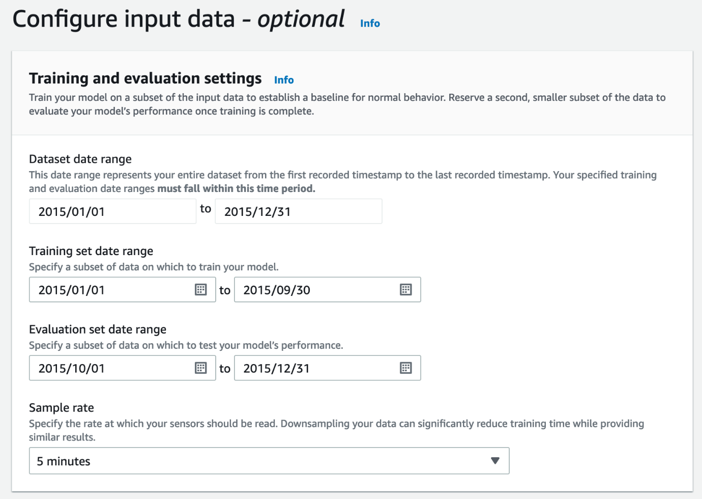
  1. In the Training and evaluation settings section, configure the model input data.

To effectively train models, the data needs to be split into separate training and evaluation sets. You can define date ranges for this split in this section, along with a sampling rate for the sensors. How do you choose this split? Consider the following:

  • Lookout for Equipment expects at least 3 months of data in the training range, but the optimal amount of data is driven by your use case. More data may be necessary to account for any type of seasonality or operational cycles your production goes through.
  • There are no constraints on the evaluation range. However, we recommend setting up an evaluation range that includes known anomalies. This way, you can test if Lookout for Equipment is able to capture any events of interest leading to these anomalies.

By specifying the sample rate, Lookout for Equipment effectively downsamples the sensor data, which can significantly reduce training time. The ideal sampling rate depends on the types of anomalies you suspect in your data: for slow-trending anomalies, selecting a sampling rate between 1–10 minutes is usually a good starting point. Choosing lower values (increasing the sampling rate) results in longer training times, whereas higher values (low sampling rate) shorten the training time at the risk of cutting out leading indicators from your data relevant to predicting the anomalies.

Configure input data for model training

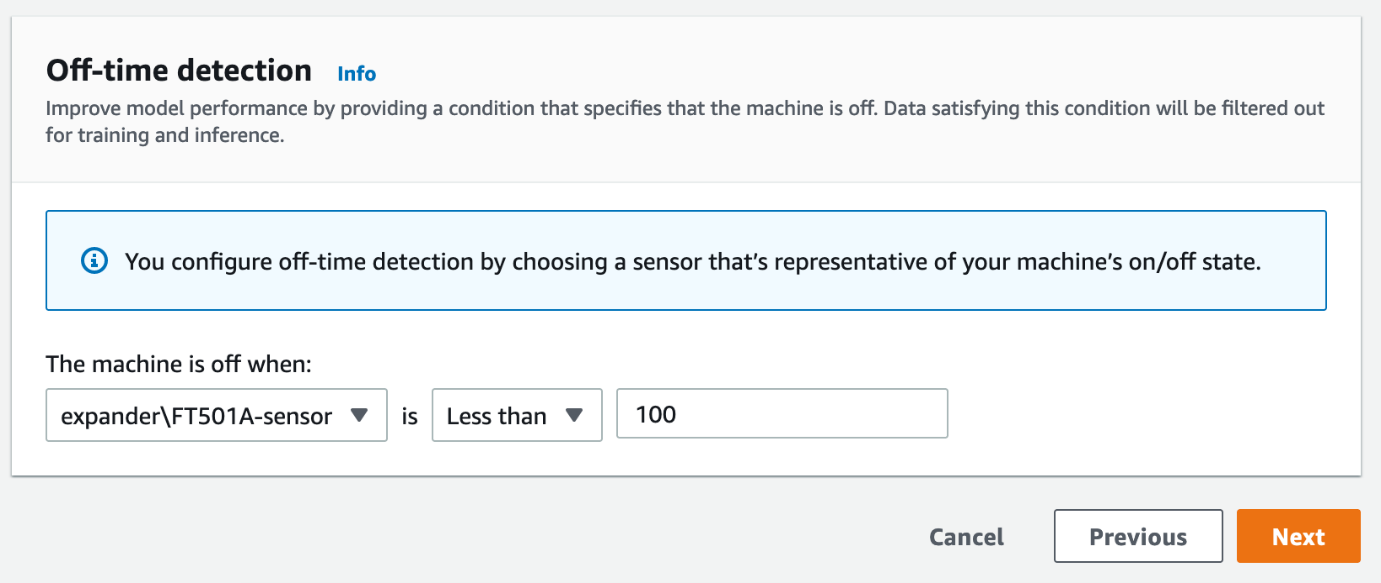
For training only on relevant portions of your data where the industrial equipment was in operation, you can perform off-time detection by selecting a sensor and defining a threshold indicating whether the equipment was in an on or off state. This is critical because it allows Lookout for Equipment to filter out time periods for training when the machine is off. This means the model learns only relevant operational states and not just when the machine is off.

  1. Specify your off-time detection, then choose Next.

Specify off time detection

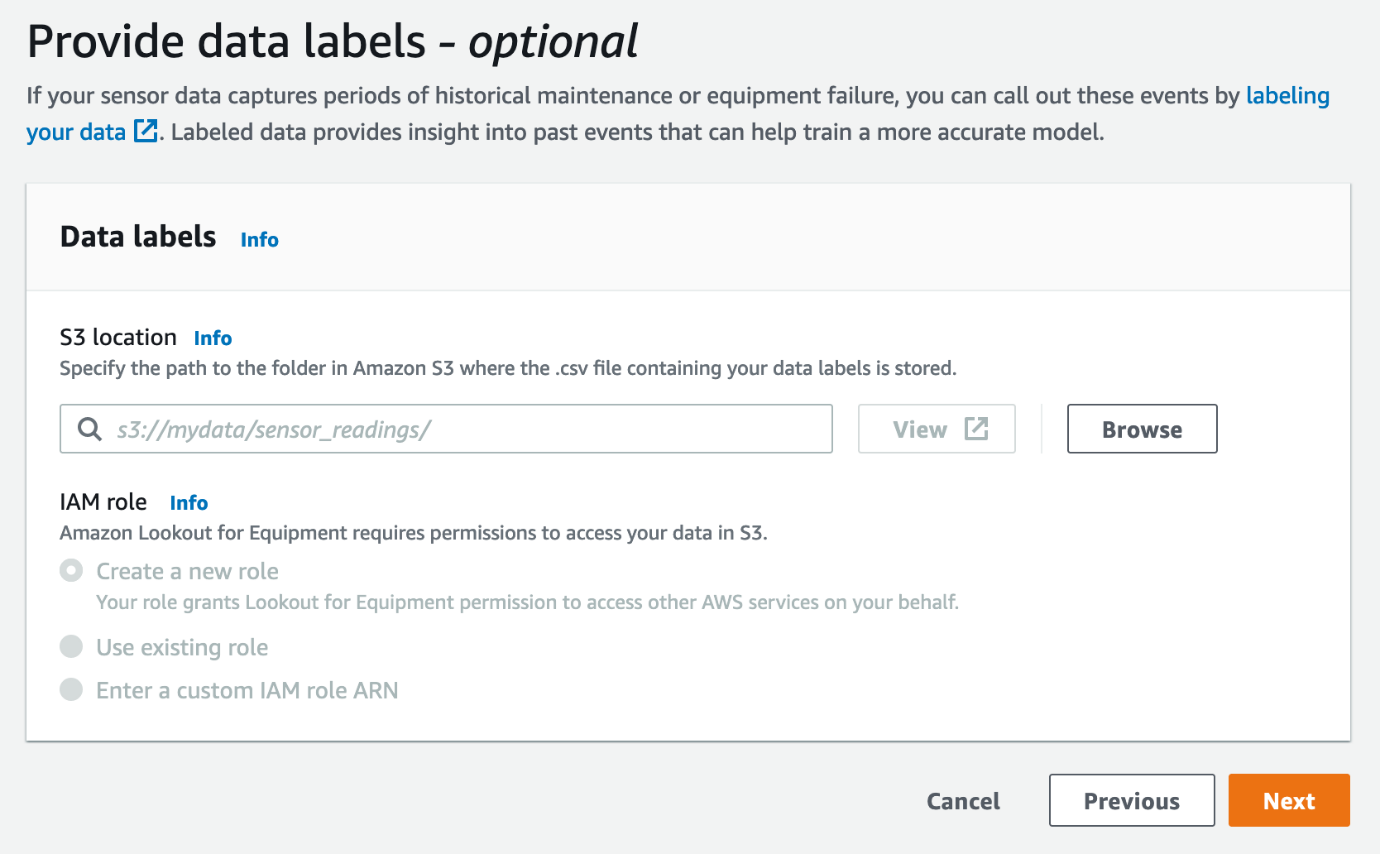
Optionally, you can provide data labels, which indicate maintenance periods or known equipment failure times. If you have such data available, you can create a CSV file with the data in a documented format, upload it to Amazon S3, and use it for model training. Providing labels can improve the accuracy of the trained model by telling Lookout for Equipment where it should expect to find known anomalies.

  1. Specify any data labels, then choose Next.

Optionally, specify data labels

  1. Review your settings in the final step. If everything looks fine, you can start the training.

Depending on the size of your dataset, the number of sensors, and the sampling rate, training the model may take a few moments or up to a few hours. For example, if you use 1 year of data at a 5-minute sampling rate with 100 sensors and no labels, training a model will take less than 15 minutes. On the other hand, if your data contains a large number of labels, training time could increase significantly. In such a situation, you can decrease training time by merging adjacent label periods to decrease their number.

You have just trained your first anomaly detection model without any ML knowledge! Now let’s look at the insights you can get from a trained model.

Evaluate a trained model

When model training has finished, you can view the model’s details by choosing View models on the project page, and then choosing the model’s name.

In addition to general information like name, status, and training time, the model page summarizes model performance data like the number of labeled events detected (assuming you provided labels), the average forewarning time, and the number of anomalous equipment events detected outside of the label ranges. The following screenshot shows an example. For better visibility, the detected events are visualized (the red bars on the top of the ribbon) along with the labeled events (the blue bars at the bottom of the ribbon).

Evaluating a model

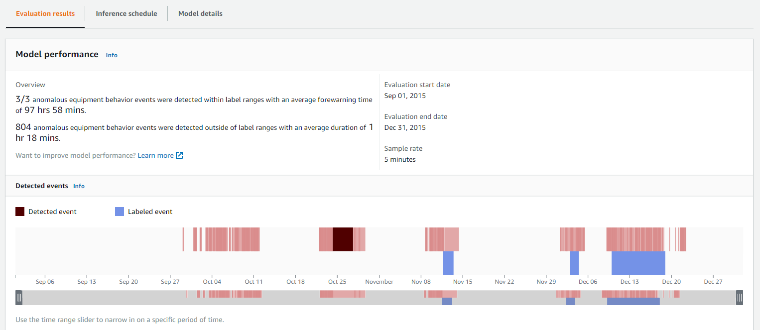
You can select detected events by choosing the red areas representing anomalies in the timeline view to get additional information. This includes:

  • The event start and end times along with its duration.
  • A bar chart with the sensors the model believes are most relevant to why an anomaly occurred. The percentage scores represent the calculated overall contribution.

Signal contribution bar charts on a selected event

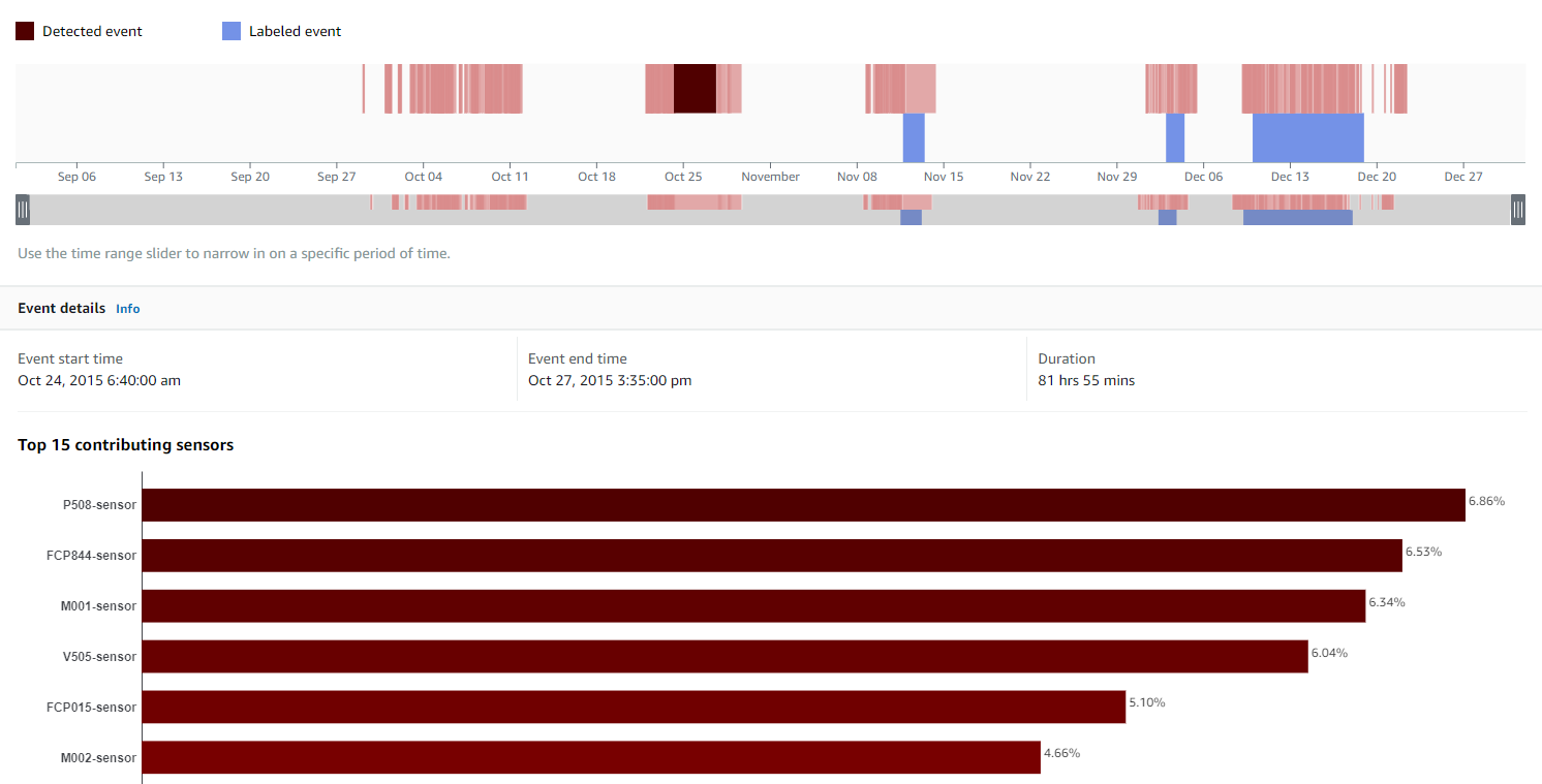
These insights allow you to work with your process or reliability engineers to do further root cause evaluation of events and ultimately optimize maintenance activities, reduce unplanned downtimes, and identify suboptimal operating conditions.

To support predictive maintenance with real-time insights (inference), Lookout for Equipment supports live evaluation of online data via inference schedules. This requires that sensor data is uploaded to Amazon S3 periodically, and then Lookout for Equipment performs inference on the data with the trained model, providing real-time anomaly scoring. The inference results, including a history of detected anomalous events, can be viewed on the Lookout for Equipment console.

7-day inference result dashboard

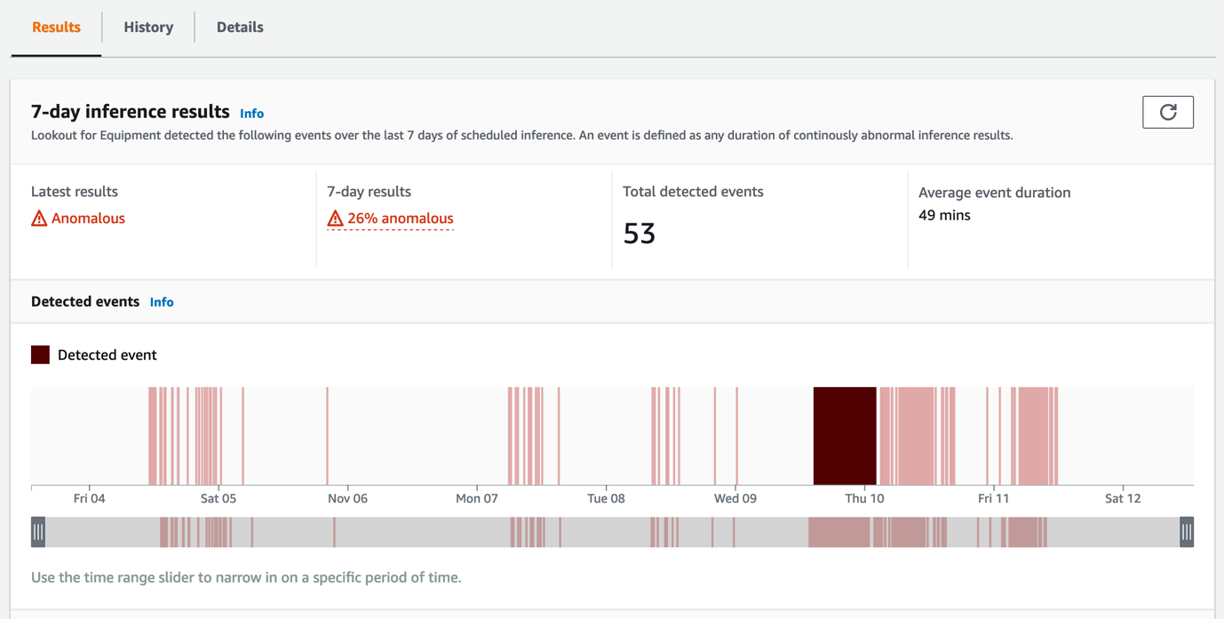
The results are also written to files in Amazon S3, allowing integration with other systems, for example a computerized maintenance management system (CMMS), or to notify operations and maintenance personnel in real time.

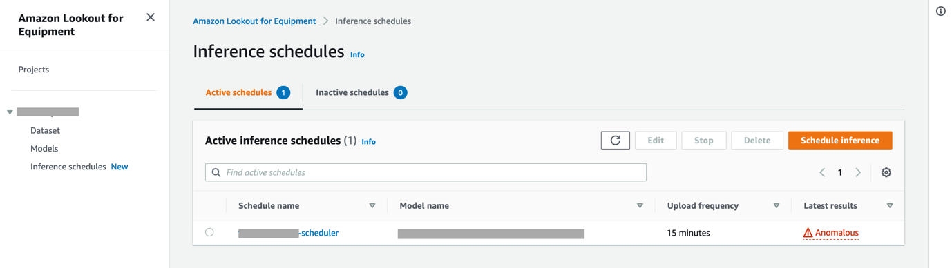
As you increase your Lookout for Equipment adoption, you’ll need to manage a larger number of models and inference schedules. To make this process easier, the Inference schedules page lists all schedulers currently configured for a project in a single view.

Inference scheduler list

Clean up

When you’re finished evaluating Lookout for Equipment, we recommend cleaning up any resources. You can delete the Lookout for Equipment project along with the dataset and any models created by selecting the project, choosing Delete, and confirming the action.

Summary

In this post, we walked through the steps of ingesting a dataset in Lookout for Equipment, training a model on it, and evaluating its performance to understand the value it can uncover for individual assets. Specifically, we explored how Lookout for Equipment can inform predictive maintenance processes that result in reduced unplanned downtime and higher OEE.

If you followed along with your own data and are excited about the prospects of using Lookout for Equipment, the next step is to start a pilot project, with the support of your IT organization, your key partners, or our AWS Professional Services teams. This pilot should target a limited number of industrial equipment and then scale up to eventually include all assets in scope for predictive maintenance.


About the authors

 Johann Füchsl is a Solutions Architect with Amazon Web Services. He guides enterprise customers in the manufacturing industry in implementing AI/ML use cases, designing modern data architectures, and building cloud-native solutions that deliver tangible business value. Johann has a background in mathematics and quantitative modeling, which he combines with 10 years of experience in IT. Outside of work, he enjoys spending time with his family and being out in nature.

Michaël Hoarau is an industrial AI/ML Specialist Solution Architect at AWS who alternates between data scientist and machine learning architect, depending on the moment. He is passionate about bringing the power of AI/ML to the shop floors of his industrial customers and has worked on a wide range of ML use cases, ranging from anomaly detection to predictive product quality or manufacturing optimization. When not helping customers develop the next best machine learning experiences, he enjoys observing the stars, traveling, or playing the piano.

Read More

What’s new in TensorFlow 2.12 and Keras 2.12?

What’s new in TensorFlow 2.12 and Keras 2.12?

Posted by the TensorFlow & Keras teams

TensorFlow 2.12 and Keras 2.12 have been released! Highlights of this release include the new Keras model saving and exporting format, the keras.utils.FeatureSpace utility, SavedModel fingerprinting, Python 3.11 wheels for TensorFlow and many more.

TensorFlow Core

SavedModel Fingerprinting

Models saved with tf.saved_model.save now come with a fingerprint file containing hashes to uniquely identify the SavedModel. Multiple fingerprints are derived from the model content, allowing you to compare the structure, graph, signatures, and weights across models. Read more about fingerprinting in the RFC and check out the read_fingerprint API and Fingerprint class.

tf.function

tf.function now uses the Python inspect library to consistently mimic the decorated function’s signature. WYSIWYG: decorated and non-decorated behavior is identical, even for complex uses like wrapping (functools.wraps) and partial application (functools.partial).

We now detect incompatible tf.function input types (such as mismatched functools.wraps calls). Additionally, we have improved type constraining logic (input_signature) for better error messages and consistency (e.g. a function with no parameters now automatically has input_signature=[]).

Additionally, we have added experimental.extension_type.as_dict() to convert tf.experimental.ExtensionTypes to Python dicts.

Keras

New model format

The biggest new Keras feature in this release is the new model export formats. We’ve completely reworked Keras saving and serialization to cleanly separate two key use cases:

1. Python saving & reloading. This is when you save a Keras model to re-instantiate it later in a Python runtime, exactly as it was. We achieve this with a new file format, called the “Keras v3” format (.keras). You can start using it by calling model.save("your_model.keras", save_format="keras_v3").


2. Model export for inference in a runtime that might not support Python at all (e.g. the TF Serving runtime). You can create a lightweight (single-file) export via model.export("your_model") – and reload it in TF Serving or Python via tf.saved_model.load("your_model"). By default, this format only preserves a single serving endpoint, the forward pass of the model, available upon reload as .serve(). Further customization is available through the keras.export.ExportArchive class.

In the 2.13 release, keras_v3 will become the default for all files with the .keras extension. The format supports non-numerical state such as vocabulary files and lookup tables, and it is easy to save custom layers with exotic state elements (such as a FIFOQueue). The format does not rely on loading arbitrary code through bytecode or pickling, so it is safe by default. This is a big advance for secure ML. Note that due to this safety-first mindset, Python lambdas are disallowed at loading time. If you want to use a lambda, and you trust the source of the model, you can pass safe_mode=False to the loading method.

The legacy formats (“h5” and “Keras SavedModel” format based on TF SavedModel) will stay supported in perpetuity. However, we recommend that you consider adopting the new Keras v3 format for richer Python-side model saving/reloading, and using export() for inference-optimized model export.

FeatureSpace

Another exciting feature is the introduction of the keras.utils.FeatureSpace utility. It enables one-step indexing and preprocessing of structured data – including feature hashing and feature crossing. See the [feature space tutorial](https://keras.io/examples/structured_data/structured_data_classification_with_feature_space/) for more information.

Like all Keras APIs, FeatureSpace is built with progressive disclosure of complexity in mind, so it is fully customizable – you can even specify custom feature types that rely on your own preprocessing layers. For instance, if you want to create a feature that encodes a text paragraph, that’s just two lines of code:

from tensorflow.keras import layers, utils custom_layer = layers.TextVectorization(output_mode="tf_idf") feature_space = utils.FeatureSpace( features={ "text": FeatureSpace.feature( preprocessor=custom_layer, dtype="string", output_mode="float" ), }, output_mode="concat", )

There are just the release highlights – there are many more Keras-related improvements included, so be sure to check out the release notes!

tf.data

Warm starting

tf.data has added support for warm-starting input processing. If warm_start=True (on tf.data.experimental.OptimizationOptions), tf.data will start preemptively start background threads during iterator creation (instead of waiting for the first call to GetNext). This allows users to improve latency to the initial GetNext call at the expense of higher memory usage.

Re-randomizing across epochs

tf.data added a new rerandomize_each_iteration argument to tf.data.Dataset.random(), to control whether the sequence of generated random numbers should be re-randomized every epoch, or not (the default behavior). If seed is set and rerandomize_each_iteration=True, random() will produce a different (deterministic) sequence of numbers every epoch. This can be useful when training over a relatively smaller number of input examples to ensure that the model doesn’t learn the sequence itself.

Infra Updates

  • Protobuf python runtime version was upgraded to 4.21.9. All protobuf *_pb2.py stubs are generated now with protoc 3.21.9. The minimal supported protobuf runtime version is 3.20.3.
  • We released Python 3.11 wheels for the TensorFlow packages with this release!
  • We removed Python 3.7 support from this version. Going forward, we will no longer release patches for Python 3.7.

      Read More

      Accelerated PyTorch 2 Transformers

      Accelerated PyTorch 2 Transformers

      The PyTorch 2.0 release includes a new high-performance implementation of the PyTorch Transformer API with the goal of making training and deployment of state-of-the-art Transformer models affordable. Following the successful release of “fastpath” inference execution (“Better Transformer”), this release introduces high-performance support for training and inference using a custom kernel architecture for scaled dot product attention (SPDA).

      You can take advantage of the new fused SDPA kernels either by calling the new SDPA operator directly (as described in the SDPA tutorial), or transparently via integration into the pre-existing PyTorch Transformer API. All features of the PyTorch Transformer API will continue to work compatibly, with many features mapped to high-performance SDPA kernels, while other features are impossible to support with higher performance (e.g., need_weights, as per below) while expanded high-performance support for other features may still be under active development.

      Similar to the “fastpath” architecture, custom kernels are fully integrated into the PyTorch Transformer API – thus, using the native Transformer and MultiHeadAttention API will enable users to transparently see significant speed improvements. Unlike the “fastpath” architecture, the newly introduced “custom kernels” support many more use cases including models using Cross-Attention, Transformer Decoders, and for training models, in addition to the existing fastpath inference for fixed and variable sequence length Transformer Encoder and Self Attention use cases.

      To take full advantage of different hardware models and Transformer use cases, multiple SDPA custom kernels are supported, with custom kernel selection logic that will pick the highest-performance kernel for a given model and hardware type. In particular, the first custom kernels included with the PyTorch 2.0 release are the Flash Attention kernel (sdpa_flash, for 16-bit floating point training and inference on Nvidia GPUs with SM80+ architecture level) and the xFormers memory-efficient attention kernel (sdpa_mem_eff, for 16-bit and 32-bit floating point training and inference on a broad range of Nvidia GPUs). A general-purpose kernel sdpa_math provides an implementation when the custom kernels are not applicable.

      As mentioned, custom kernels provide a wider range of support for execution scenarios To ensure efficient execution (e,g., to use GPU tensor cores), model configurations need to meet a small number of requirements. This list of requirements will evolve over time, prospectively relaxing constraints limiting the usage of currently supported custom kernels, or providing additional kernels in the future.

      For the most up to date list of custom kernels and dispatch constraints, you can refer to sdp_utils.h. As of PyTorch 2.0, the existing fused SDPA kernels have the following constraints:

      • Flash Attention only supports 16 bit floating point data types (float16 and bfloat16).
      • The head dimension must be a multiple of 8 for 16-bit floating point numbers and a multiple of 4 for 32-bit floating point numbers. At present, the maximum head_dim support for the Flash Attention custom kernel is 128.
      • The CUDA architecture level must be sm5x or better for the mem_efficient kernel, and sm80 for Flash Attention.
      • Flash Attention supports arbitrary dropout, in PyTorch 2.0 the mem_efficient kernel does not support dropout (i.e., dropout must be set to zero for this kernel to be selected in PyTorch 2.0).
      • To support variable-sequence length batches, all SDPA kernels support Nested Tensor inputs that combine input data and padding information using variable sequence length tensors for forward. (You can find more information about Nested Tensors in the Nested Tensor tutorial.)
      • You can specify both a key_padding_mask and an attn_mask by combining them before passing them to the SDPA operator. In particular, you can use the per-batch-element key padding mask of the nn.Transformer API to implement training for variable-sequence length inputs in a batch.
      • At present, the only attention mask supported by fused kernel implementation is the causal mask commonly used for training. To specify the causal mask in custom kernels, it must be specified with the is_causal boolean and attn_mask must be None.
      • Support for Nested Tensors is still under development. Specifically, in PyTorch 2.0, only the sdpa_math kernel supports training with Nested Tensors. Also, PyTorch 2.0 does not support Nested Tensors as part of code being compiled with torch.compile().
      • The SDPA operator does not support returning averaged attention weights because computing them defeats the optimizations that enabled fused kernels to execute more efficiently. The argument need_weights for torch.nn.MultiheadAttention’s forward function defaults to True. In order to use the fused kernels, need_weights needs to be set to need_weights=False.

      We find that an attention mask is rarely used in real-world applications, except for the causal mask during training. Consequently, we reduce kernel complexity and compute cost by building in the option to use a causal mask as attention mask, and select this new capability with the is_causal parameter introduced in conjunction with the new SDPA operator.

      Providing the is_causal Boolean flag for the frequently used causal mask also obviates the expensive and memory-intensive allocation of a causal mask, increasing training memory efficiency by allowing more memory to be used for large batch sizes, and reduce memory bandwidth and cache contention – which are both at a premium in GPU accelerators – by not needing to load an attention mask tensor.

      If the constraints of none of the available custom kernels are met, then training falls back to using the default sdpa_math kernel, implementing the mathematical equations for scaled dot product attention using a sequence of PyTorch operator to implement SDPA. This is the most general “catch-all” fallback kernel to ensure successful training for all models.

      In addition to the existing Transformer API, model developers may also use the scaled dot product attention kernels directly by calling the new scaled_dot_product_attention() operator. This operator may be used to efficiently implement multi-head attention by combining it with in-projection and outprojection, as described in the SDPA tutorial.

      In addition to adding custom kernels, Accelerated PyTorch 2 Transformers are integrated with PyTorch 2.0 compilation. To use your model while benefiting from the additional acceleration of PT2-compilation (for inference or training), pre-process the model with

      model = torch.compile(model)
      

      We have achieved major speedups for training transformer models and in particular large language models with Accelerated PyTorch 2 Transformers using a combination of custom kernels and torch.compile().

      Better Transformer chart
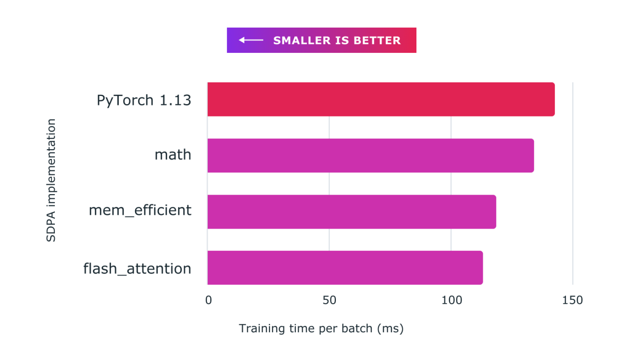
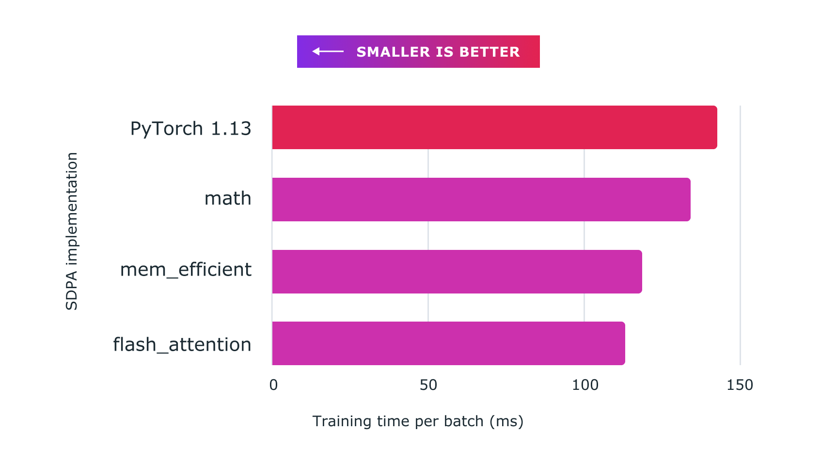
Figure: Using scaled dot product attention with custom kernels and torch.compile delivers significant speedups for training large language models, such as for nanoGPT shown here.

      Finally, because the custom kernels are much more memory efficient, try to increase the size of training batches to achieve faster training with increased batch size.

      In addition to automatic kernel selection, a context manager enables developers to override the kernel selection algorithm – this is not required for day to day operation, but enables developers to debug their code as well as enable performance engineers to override kernel selection. The SDPA tutorial provides additional information on using the SDPA context manager.

      In addition to availability as part of the nn.Transformer API, Accelerated PyTorch 2 Transformer custom kernels are also available in conjunction with the torchtext, torchvision, and fairseq domain libraries with the launch of PyTorch 2.0.

      Read More

      PRESTO – A multilingual dataset for parsing realistic task-oriented dialogues

      PRESTO – A multilingual dataset for parsing realistic task-oriented dialogues

      Virtual assistants are increasingly integrated into our daily routines. They can help with everything from setting alarms to giving map directions and can even assist people with disabilities to more easily manage their homes. As we use these assistants, we are also becoming more accustomed to using natural language to accomplish tasks that we once did by hand.

      One of the biggest challenges in building a robust virtual assistant is identifying what a user wants and what information is needed to perform the task at hand. In the natural language processing (NLP) literature, this is mainly framed as a task-oriented dialogue parsing task, where a given dialogue needs to be parsed by a system to understand the user intent and carry out the operation to fulfill that intent. While the academic community has made progress in handling task-oriented dialogue thanks to custom purpose datasets, such as MultiWOZ, TOP, SMCalFlow, etc., progress is limited because these datasets lack typical speech phenomena necessary for model training to optimize language model performance. The resulting models often underperform, leading to dissatisfaction with assistant interactions. Relevant speech patterns might include revisions, disfluencies, code-mixing, and the use of structured context surrounding the user’s environment, which might include the user’s notes, smart home devices, contact lists, etc.

      Consider the following dialogue that illustrates a common instance when a user needs to revise their utterance:

      A dialogue conversation with a virtual assistant that includes a user revision.

      The virtual assistant misunderstands the request and attempts to call the incorrect contact. Hence, the user has to revise their utterance to fix the assistant’s mistake. To parse the last utterance correctly, the assistant would also need to interpret the special context of the user — in this case, it would need to know that the user had a contact list saved in their phone that it should reference.

      Another common category of utterance that is challenging for virtual assistants is code-mixing, which occurs when the user switches from one language to another while addressing the assistant. Consider the utterance below:

      A dialogue denoting code-mixing between English and German.

      In this example, the user switches from English to German, where “vier Uhr” means “four o’clock” in German.

      In an effort to advance research in parsing such realistic and complex utterances, we are launching a new dataset called PRESTO, a multilingual dataset for parsing realistic task-oriented dialogues that includes roughly half a million realistic conversations between people and virtual assistants. The dataset spans six different languages and includes multiple conversational phenomena that users may encounter when using an assistant, including user-revisions, disfluencies, and code-mixing. The dataset also includes surrounding structured context, such as users’ contacts and lists associated with each example. The explicit tagging of various phenomena in PRESTO allows us to create different test sets to separately analyze model performance on these speech phenomena. We find that some of these phenomena are easier to model with few-shot examples, while others require much more training data.

      Dataset characteristics

      1. Conversations by native speakers in six languages
        All conversations in our dataset are provided by native speakers of six languages — English, French, German, Hindi, Japanese, and Spanish. This is in contrast to other datasets, such as MTOP and MASSIVE, that translate utterances only from English to other languages, which does not necessarily reflect the speech patterns of native speakers in non-English languages.
      2. Structured context
        Users often rely on the information stored in their devices, such as notes, contacts, and lists, when interacting with virtual assistants. However, this context is often not accessible to the assistant, which can result in parsing errors when processing user utterances. To address this issue, PRESTO includes three types of structured context, notes, lists, and contacts, as well as user utterances and their parses. The lists, notes, and contacts are authored by native speakers of each language during data collection. Having such context allows us to examine how this information can be used to improve performance on parsing task-oriented dialog models.
        Each example in PRESTO consists of: Inputs — A user’s virtual state (context), one or more user utterances, and the corresponding virtual assistant responses (dialogue). Output — The semantic parsing of the last user utterance in the dialogue (parse).
      3. User revisions
        It is common for a user to revise or correct their own utterances while speaking to a virtual assistant. These revisions happen for a variety of reasons — the assistant could have made a mistake in understanding the utterance or the user might have changed their mind while making an utterance. One such example is in the figure above. Other examples of revisions include canceling one’s request (‘’Don’t add anything.”) or correcting oneself in the same utterance (“Add bread — no, no wait — add wheat bread to my shopping list.”). Roughly 27% of all examples in PRESTO have some type of user revision that is explicitly labeled in the dataset.
      4. Code-mixing
        As of 2022, roughly 43% of the world’s population is bilingual. As a result, many users switch languages while speaking to virtual assistants. In building PRESTO, we asked bilingual data contributors to annotate code-mixed utterances, which amounted to roughly 14% of all utterances in the dataset.
        Examples of Hindi-English, Spanish-English, and German-English code-switched utterances from PRESTO.
      5. Disfluencies
        Disfluencies, like repeated phrases or filler words, are ubiquitous in user utterances due to the spoken nature of the conversations that the virtual assistants receive. Datasets such as DISFL-QA note the lack of such phenomena in existing NLP literature and contribute towards the goal of alleviating that gap. In our work, we include conversations targeting this particular phenomenon across all six languages.
        Examples of utterances in English, Japanese, and French with filler words or repetitions.

      Key findings

      We performed targeted experiments to focus on each of the phenomena described above. We ran mT5-based models trained using the PRESTO dataset and evaluated them using an exact match between the predicted parse and the human annotated parse. Below we show the relative performance improvements as we scale the training data on each of the targeted phenomena — user revisions, disfluencies, and code-mixing.

      K-shot results on various linguistic phenomena and the full test set across increasing training data size.

      The k-shot results yield the following takeaways:

      1. Zero-shot performance on the marked phenomenon is poor, emphasizing the need for such utterances in the dataset to improve performance.
      2. Disfluencies and code-mixing have a much better zero-shot performance than user-revisions (over 40 points difference in exact-match accuracy).

      We also investigate the difference between training monolingual and multilingual models on the train set and find that with fewer data multilingual models have an advantage over monolingual models, but the gap shrinks as the data size is increased.

      Additional details on data quality, data collection methodology, and modeling experiments can be found in our paper.

      Conclusion

      We created PRESTO, a multilingual dataset for parsing task-oriented dialogues that includes realistic conversations representing a variety of pain points that users often face in their daily conversations with virtual assistants that are lacking in existing datasets in the NLP community. PRESTO includes roughly half a million utterances that are contributed by native speakers of six languages — English, French, German, Hindi, Japanese, and Spanish. We created dedicated test sets to focus on each targeted phenomenon — user revisions, disfluencies, code-mixing, and structured context. Our results indicate that the zero-shot performance is poor when the targeted phenomenon is not included in the training set, indicating a need for such utterances to improve performance. We notice that user revisions and disfluencies are easier to model with more data as opposed to code-mixed utterances, which are harder to model, even with a high number of examples. With the release of this dataset, we open more questions than we answer and we hope the research community makes progress on utterances that are more in line with what users are facing every day.

      Acknowledgements

      It was a privilege to collaborate on this work with Waleed Ammar, Siddharth Vashishtha, Motoki Sano, Faiz Surani, Max Chang, HyunJeong Choe, David Greene, Kyle He, Rattima Nitisaroj, Anna Trukhina, Shachi Paul, Pararth Shah, Rushin Shah, and Zhou Yu. We’d also like to thank Tom Small for the animations in this blog post. Finally, a huge thanks to all the expert linguists and data annotators for making this a reality.

      Read More

      Detecting novel systemic biomarkers in external eye photos

      Detecting novel systemic biomarkers in external eye photos

      Last year we presented results demonstrating that a deep learning system (DLS) can be trained to analyze external eye photos and predict a person’s diabetic retinal disease status and elevated glycated hemoglobin (or HbA1c, a biomarker that indicates the three-month average level of blood glucose). It was previously unknown that external eye photos contained signals for these conditions. This exciting finding suggested the potential to reduce the need for specialized equipment since such photos can be captured using smartphones and other consumer devices. Encouraged by these findings, we set out to discover what other biomarkers can be found in this imaging modality.

      In “A deep learning model for novel systemic biomarkers in photos of the external eye: a retrospective study”, published in Lancet Digital Health, we show that a number of systemic biomarkers spanning several organ systems (e.g., kidney, blood, liver) can be predicted from external eye photos with an accuracy surpassing that of a baseline logistic regression model that uses only clinicodemographic variables, such as age and years with diabetes. The comparison with a clinicodemographic baseline is useful because risk for some diseases could also be assessed using a simple questionnaire, and we seek to understand if the model interpreting images is doing better. This work is in the early stages, but it has the potential to increase access to disease detection and monitoring through new non-invasive care pathways.

      A model generating predictions for an external eye photo.

      Model development and evaluation

      To develop our model, we worked with partners at EyePACS and the Los Angeles County Department of Health Services to create a retrospective de-identified dataset of external eye photos and measurements in the form of laboratory tests and vital signs (e.g., blood pressure). We filtered down to 31 lab tests and vitals that were more commonly available in this dataset and then trained a multi-task DLS with a classification “head” for each lab and vital to predict abnormalities in these measurements.

      Importantly, evaluating the performance of many abnormalities in parallel can be problematic because of a higher chance of finding a spurious and erroneous result (i.e., due to the multiple comparisons problem). To mitigate this, we first evaluated the model on a portion of our development dataset. Then, we narrowed the list down to the nine most promising prediction tasks and evaluated the model on our test datasets while correcting for multiple comparisons. Specifically, these nine tasks, their associated anatomy, and their significance for associated diseases are listed in the table below.

      Prediction task       Organ system       Significance for associated diseases      
      Albumin < 3.5 g/dL       Liver/Kidney       Indication of hypoalbuminemia, which can be due to decreased production of albumin from liver disease or increased loss of albumin from kidney disease.      
      AST > 36.0 U/L       Liver      

      Indication of liver disease (i.e., damage to the liver or biliary obstruction), commonly caused by viral infections, alcohol use, and obesity.

           
      Calcium < 8.6 mg/dL       Bone / Mineral       Indication of hypocalcemia, which is most commonly caused by vitamin D deficiency or parathyroid disorders.      
      eGFR < 60.0 mL/min/1.73 m2       Kidney      

      Indication of chronic kidney disease, most commonly due to diabetes and high blood pressure.

           
      Hgb < 11.0 g/dL       Blood count       Indication of anemia which may be due to blood loss, chronic medical conditions, or poor diet.      
      Platelet < 150.0 103/µL       Blood count      

      Indication of thrombocytopenia, which can be due to decreased production of platelets from bone marrow disorders, such as leukemia or lymphoma, or increased destruction of platelets due to autoimmune disease or medication side effects.

           
      TSH > 4.0 mU/L       Thyroid       Indication of hypothyroidism, which affects metabolism and can be caused by many different conditions.      
      Urine albumin/creatinine ratio (ACR) ≥ 300.0 mg/g       Kidney      

      Indication of chronic kidney disease, most commonly due to diabetes and high blood pressure.

           
      WBC < 4.0 103/µL       Blood count       Indication of leukopenia which can affect the body’s ability to fight infection.      

      Key results

      As in our previous work, we compared our external eye model to a baseline model (a logistic regression model taking clinicodemographic variables as input) by computing the area under the receiver operator curve (AUC). The AUC ranges from 0 to 100%, with 50% indicating random performance and higher values indicating better performance. For all but one of the nine prediction tasks, our model statistically outperformed the baseline model. In terms of absolute performance, the model’s AUCs ranged from 62% to 88%. While these levels of accuracy are likely insufficient for diagnostic applications, it is in line with other initial screening tools, like mammography and pre-screening for diabetes, used to help identify individuals who may benefit from additional testing. And as a non-invasive accessible modality, taking photographs of the external eye may offer the potential to help screen and triage patients for confirmatory blood tests or other clinical follow-up.

      Results on the EyePACS test set, showing AUC performance of our DLS compared to a baseline model. The variable “n” refers to the total number of datapoints, and “N” refers to the number of positives. Error bars show 95% confidence intervals computed using the DeLong method. Indicates that the target was pre-specified as secondary analysis; all others were pre-specified as primary analysis.

      The external eye photos used in both this and the prior study were collected using table top cameras that include a head rest for patient stabilization and produce high quality images with good lighting. Since image quality may be worse in other settings, we wanted to explore to what extent the DLS model is robust to quality changes, starting with image resolution. Specifically, we scaled the images in the dataset down to a range of sizes, and measured performance of the DLS when retrained to handle the downsampled images.

      Below we show a selection of the results of this experiment (see the paper for more complete results). These results demonstrate that the DLS is fairly robust and, in most cases, outperforms the baseline model even if the images are scaled down to 150×150 pixels. This pixel count is under 0.1 megapixels, much smaller than the typical smartphone camera.

      Effect of input image resolution. Top: Sample images scaled to different sizes for this experiment. Bottom: Comparison of the performance of the DLS (red) trained and evaluated on different image sizes and the baseline model (blue). Shaded regions show 95% confidence intervals computed using the DeLong method.

      Conclusion and future directions

      Our previous research demonstrated the promise of the external eye modality. In this work, we performed a more exhaustive search to identify the possible systemic biomarkers that can be predicted from these photos. Though these results are promising, many steps remain to determine whether technology like this can help patients in the real world. In particular, as we mention above, the imagery in our studies were collected using large tabletop cameras in a setting that controlled factors such as lighting and head positioning. Furthermore, the datasets used in this work consist primarily of patients with diabetes and did not have sufficient representation of a number of important subgroups – more focused data collection for DLS refinement and evaluation on a more general population and across subgroups will be needed before considering clinical use.

      We are excited to explore how these models generalize to smartphone imagery given the potential reach and scale that this enables for the technology. To this end, we are continuing to work with our co-authors at partner institutions like Chang Gung Memorial Hospital in Taiwan, Aravind Eye Hospital in India, and EyePACS in the United States to collect datasets of imagery captured on smartphones. Our early results are promising and we look forward to sharing more in the future.

      Acknowledgements

      This work involved the efforts of a multidisciplinary team of software engineers, researchers, clinicians and cross functional contributors. Key contributors to this project include: Boris Babenko, Ilana Traynis, Christina Chen, Preeti Singh, Akib Uddin, Jorge Cuadros, Lauren P. Daskivich, April Y. Maa, Ramasamy Kim, Eugene Yu-Chuan Kang, Yossi Matias, Greg S. Corrado, Lily Peng, Dale R. Webster, Christopher Semturs, Jonathan Krause, Avinash V Varadarajan, Naama Hammel and Yun Liu. We also thank Dave Steiner, Yuan Liu, and Michael Howell for their feedback on the manuscript; Amit Talreja for reviewing code for the paper; Elvia Figueroa and the Los Angeles County Department of Health Services Teleretinal Diabetic Retinopathy Screening program staff for data collection and program support; Andrea Limon and Nikhil Kookkiri for EyePACS data collection and support; Dr. Charles Demosthenes for extracting the data and Peter Kuzmak for getting images for the VA data. Last but not least, a special thanks to Tom Small for the animation used in this blog post.

      Read More

      Towards Behavior-Driven AI Development

      Towards Behavior-Driven AI Development

      Figure 1: Behavior-driven AI development centers model iteration on evaluating and improving specific real-world use cases.

      It has never been easier to prototype AI-driven systems. With a bit of programming knowledge and a couple of hours, you can spin up a chatbot for your notes, a text-based image editor, or a tool for summarizing customer feedback. But play around with your prototype for a bit, and you might find that it doesn’t work as well as you first expected. Your system might make up facts or respond with racist suggestions. How would you evaluate your model and predict its performance in deployment?

      The canonical process for benchmarking AI systems revolves around model-centric metrics. Calculate a metric (F1-score, precision, etc.), and if it increases, you are going in the right direction. But these metrics are oversimplified objectives that sand away the complexity of model behavior and cannot fully represent a model’s performance. A metric may tell you how well your model can predict the next word in a sentence, but it won’t tell you how factually accurate, logical, or fair your model is across diverse, real-world use cases. Generative AI systems such as ChatGPT or Stable Diffusion make evaluation even more challenging since there are no well-defined metrics that can summarize their performance.

      When creating deployed AI products, practitioners instead focus on the specific use cases their customers have and whether or not their models are fulfilling them. In interviews with 18 AI practitioners, we found that they constantly collect user feedback and develop “golden test sets” of behaviors that they expect deployed models to have. We term this behavior-driven AI development, a development process focused on evaluating and updating models to improve performance on real-world use cases. While chatbot A might sound more human-like, a practitioner will deploy chatbot B if it produces concise and accurate answers that customers prefer.

      The landscape of AI evaluation tools primarily revolves around model-centric metrics that do not capture important behaviors like these chatbot characteristics. While there are specific tools for behavior-driven development, such as fairness toolkits and robustness analysis libraries, practitioners end up cobbling together disparate tools into ad-hoc scripts or computational notebooks that are hard to maintain and reproduce.

      I believe that there are a set of abstractions that can unify AI evaluation in line with model use cases in practice. This philosophy revolves around model behaviors: metrics summarizing patterns of output on subgroups of instances. This simple concept can encode any model evaluation or analysis, from fairness audits to language model hallucinations. We show what this can look like with Zeno, an interactive platform we built for behavior-driven development that supports interactive data exploration, slicing, and reporting. By investigating their own models using Zeno, practitioners have been able to pinpoint significant and actionable issues such as biases and systematic failures. 

      What is model behavior?

      The dictionary describes behavior as anything that an organism does involving action and response to stimulation. In the case of AI systems, model behavior is a specific pattern of output for a semantically meaningful subgroup of input data (stimulus). By semantically meaningful, I mean subgroups that can be described with human-interpretable concepts, such as “audio with noise in the background” or “people who identify as women.” Similarly, a pattern of output could be “high audio transcription error” or “low loan approval rate.” 

      Behaviors can be quantified as metrics on subgroups of data, often using the same metrics as are used for model-centric evaluation. But unlike summary metrics across an entire dataset, metrics in behavior-centric development quantify specific patterns of behavior, like how often an image generation model produces unintelligible text. Tests of model behaviors are like exams for specific subjects, while summary metrics resemble IQ tests.

      Figure 2. How model behaviors are defined from a dataset. Behaviors are subgroups of data (typically defined by combinations of metadata) quantified by a specific metric. For the example behavior of “blurry text” from a text-to-image model, a metadata column for “images with text” could be used to create a subgroup on which a metric measuring the clarity of text can be calculated.

      Model behaviors are a relatively simple concept, but encoding behaviors can be challenging in practice. Practitioners may not have enough data to validate or fix important model behaviors and have to collect or generate more data. If they have extensive data, they need ways to subdivide it into meaningful groups of instances – how do I find all images that have text? Lastly, for each subgroup, practitioners have to derive the appropriate metrics to quantify the prevalence of behavior – how do I detect blurry text? Succinctly, behavior-driven development requires sufficient data that is representative of expected behaviors and metadata for defining and quantifying the behaviors.

      A platform for behavior-driven AI development

      The beauty of a behavior-based framing on AI development is that it is still data and model agnostic. While the specific behaviors for each ML task will be vastly different, subgroups of data and metrics are universal concepts.

      To test this theory, we built a platform for behavior-driven AI development called Zeno. Zeno is a platform that empowers users to explore data and model outputs, interactively create subgroups of data, and calculate and quantify model behaviors. Zeno consists of a Python API for scaffolding the data needed for analysis and a user interface for interactively creating subgroups and evaluating behaviors.

      Figure 3. The Zeno interface shown for the Imagenette dataset and image classification. The right side has the instance view showing the input images and model outputs. The left side shows distributions for the dataset’s metadata, which has been interactively filtered to show images of English Springer Spaniels.

      The Python API is a set of decorator functions (wrappers on user-defined functions) that can be used to plug in ML models and derive metadata features and metrics from input data. Since the decorators are generic wrappers, Zeno supports any Python-based model, processing function, or metric. Zeno preprocesses the input data with these functions, which it passes into the UI for analysis.

      Zeno’s UI is the primary interface for behavior-driven evaluation. It allows users to interactively explore and filter their data, create slices, calculate metrics, and create exportable visualizations. On the right side of the UI is Zeno’s instance view, where users can explore the raw data on which the model is being evaluated. In addition to the standard list view, users can also see the data in a table or a 2D scatterplot representation. The left side of the interface holds the metadata panel. All the metadata columns that either came with the dataset or were generated with the Python API have their distributions displayed in the panel. Users can interactively filter the distributions to update the instance view and create named subgroups.

      The UI also has a report page for creating interactive summary visualizations of behaviors. For example, a user could create a bar chart comparing the performance of three models across ten different slices. Or they could create a line chart showing how a model performs on data slices from each day of data. These visualizations can be exported or shared directly with other stakeholders.

      Figure 4: With Zeno, users can interactively filter their data to create slices and calculate subgroup metrics. They can also use the 2D projection to find new areas of data where their model is underperforming. In this example, a user is exploring the CIFAR-10 classification model. They first filter the dataset to compare low versus high brightness images, finding a significant difference in accuracy between the two groups. They then find a group of instances with high error in the projection view, which is mostly made up of birds in the sky being misclassified as airplanes.

      Case Studies

      We have worked with various ML practitioners to apply Zeno to the models and tasks on which they work. Using Zeno, practitioners found significant model issues and areas for improvement, including gender biases and regional model disparities.

      Audio transcription. This first case study I ran myself after I heard that OpenAI released a new speech-to-text model, Whisper, with state-of-the-art performance. I was curious how the model compared to some existing off-the-shelf transcription models. Instead of looking at aggregate metrics, I ran the models on the Speech Accent Archive dataset, which has speakers worldwide saying the same phrase. By filtering the dataset’s extensive metadata, I found that the models perform worse for English speakers who learned the language later in life and speakers from countries where English is not the native language.

      Figure 5. (left) The average word error rate (WER) for both models across different ages when participants started learning English. (right) The average WER of the Silero and Whisper transcription models across speakers from different continents.
      Charts exported directly from the Zeno Report UI. 

      Cancer classification. In another case study, we worked with a researcher who wanted to improve a breast cancer classifier for mammogram images. Since the data was anonymized and lacked meaningful metadata, the practitioner wrote dozens of functions using a Python library to extract meaningful metadata features. By exploring the distributions, they found that images with higher “entropy” correlating with denser breast tissue had a significantly higher error rate than images with lower entropy, or less dense, tissue. This finding matches performance differences in human radiologists, who also perform worse for images of denser breast tissue since it makes it harder to detect lesions.

      Low density (4937)
      entropy < 2.75 &&
      gray level variance < 2.5
      High density (656)
      entropy > 2.75 &&
      gray level variance > 2.5
      AUC 0.86 0.76
      Figure 6. The breast cancer classification model performed significantly worse for high-density images (described by high entropy and gray level variance metadata levels) compared to the low-density images. (left, low density, right, high density).

      Image generation. Models with complex outputs often do not have clearly defined metrics, including text-to-image generation models such as DALL*E and Stable Diffusion. We can instead look at metrics that measure specific behaviors. In this example, a practitioner we worked with was exploring the DiffusionDB dataset, which has over two million prompt-image pairs from the Stable Diffusion model. The dataset also has metadata for how NSFW or inappropriate the prompts and images are. This data was used to derive an “average NSFW” metric, which can show us interesting potential biases in the model. For example, the participant compared the images generated using prompts with the word “boy” versus “girl” and found that prompts with “girl” generated images with a significantly higher NSFW level than prompts with “boy”, showing potential biases in the types of images created by the model.

      Figure 7. Given similar or less inappropriate prompts, the images generated with stable diffusion are much more inappropriate (NSFW) for prompts with “girl” or “woman” than “boy” or “man”.
      Charts exported directly from the Zeno Report UI. 

      Discussion and Opportunities

      Model iteration is still a primarily reactive process of finding and defining behaviors after a model has been deployed and the customer complaints start rolling in. There remains significant room for improving this process, from making it easier to ideate model behaviors to tracking model changes over time.

      Discovering behaviors. While practitioners often need a model to discover the behaviors the model should have, methods for defining expected model behaviors before deployment can prevent serious real-world model issues.  For example, crowdsourcing techniques for eliciting potential edge cases could preemptively catch model errors. Algorithmic methods that find clusters of data with high error have also shown promise for surfacing problematic behaviors.

      Data discovery and generation. Having high-quality, representative data remains a persistent obstacle for behavioral evaluation. In some domains with ample data, such as natural images, methods like Stable Diffusion have shown promise for generating new data for evaluation or training. In less data-rich domains, techniques for searching through large unlabeled datasets, such as text-based image search, can surface valuable data for evaluation and retraining. It is also challenging to derive metadata from instances for creating subgroups and calculating metrics. While it can be easy to generate metadata for simple concepts like “image brightness,” many behaviors are defined by complex metadata such as “images with a person wearing clear glasses” that cannot be encoded by a simple function. Foundation models have shown some promise in using text-based descriptions to generate complex metadata and metrics.

      Model comparison. Models are almost never one-off jobs and can be updated daily or weekly. While it is easy to compare aggregate metrics, it can be challenging to compare model performance in behavior-driven development. To pick between models, users may have to compare dozens of behaviors and qualitative insights. Improved visual encodings or intelligent recommendations of model differences could help users make informed decisions and deploy the right models.

      Fixing behaviors. Discovering and encoding behaviors is one thing, but fixing behaviors is another massive challenge. A common approach to fixing issues is to gather more data and retrain the model, but this process can lead to catastrophic forgetting and regressions. There are recent techniques that align well with behavior-driven development, such as slice-based learning, which can selectively fix model behaviors without new data.

      Conclusion

      There is significant excitement for this new era of AI systems. But along with their growing capability, the complexity of their behavior is also increasing. We need powerful tools to empower behavior-driven development and ensure we build intelligent systems that align with human values. Zeno provides a general-purpose platform that empowers users to do this deep evaluation across the diverse tasks of modern AI. Learn more about Zeno at zenoml.com, read the full paper, or reach out if you would like to use Zeno for your models!

      Acknowledgments

      I’d like to thank Will Epperson, Jason I. Hong, Yi-Cheng Huang, Misha Khodak, Adam Perer, Venkat Sivaraman, Ameet Talwalkar, and Kristen Vossler for their thoughtful feedback and advice.

      Read More