Monthly Archives: June 2023

Machine learning (ML) administrators play a critical role in maintaining the security and integrity of ML workloads. Their primary focus is to ensure that users operate with the utmost security, adhering to the principle of least privilege. However, accommodating the diverse needs of different user personas and creating appropriate permission policies can sometimes impede agility. To address this challenge, AWS introduced Amazon SageMaker Role Manager in December 2022. SageMaker Role Manager is a powerful tool can you can use to swiftly develop persona-based roles, which can be easily customized to meet specific requirements.

With SageMaker Role Manager, administrators can efficiently define persona-based roles tailored to distinct user groups. This approach ensures that individuals have access only to the resources and actions essential for their tasks, reducing the risk of unauthorized actions or breaches. SageMaker Role Manager also allows for fine-grained customization. ML administrators can tailor the roles to meet specific requirements by modifying the permissions associated with each persona. This flexibility ensures that the permissions align precisely with the tasks and responsibilities of individual users, providing a robust security framework while accommodating unique use cases.

SageMaker Role Manager is currently available on the Amazon SageMaker console of all commercial Regions. Today, we are launching the ability to define customized permissions in minutes with SageMaker Role Manager via the AWS Cloud Development Kit (AWS CDK). This addresses a critical obstacle to wider adoption because ML administrators can now automate their tasks programmatically. With the power of the AWS CDK, ML administrators can streamline workflows, reduce manual efforts, and ensure consistency in managing permissions for their ML infrastructure.

Solution overview

With the release of the SageMaker Role Manager CDK, we are launching two new infrastructure as code (IaC) capabilities:

• Create fine-grained permissions for ML personas
• Create fine-grained permissions for automated jobs through Amazon SageMaker Pipelines, AWS Lambda, and other AWS services

You can create fine-grained AWS Identity and Access Management (IAM) roles for ML personas such as data scientist, ML engineer, or data engineer. SageMaker Role Manager offers predefined personas and ML activities combined to streamline your permission generation process, allowing your ML practitioners to perform their responsibilities with the least privilege permissions. For secure access to your ML resources, SageMaker Role Manager allows you to specify networking and encryption permissions for Amazon Virtual Private Cloud (Amazon VPC) resources and AWS Key Management Service (AWS KMS) encryption keys. Furthermore, you can customize permissions by attaching your own customer managed policies.

The SageMaker Role Manager CDK lets you define custom permissions for SageMaker users in minutes. It comes with a set of predefined policy templates for different personas and ML activities. Personas represent the different types of users that need permissions to perform ML activities in SageMaker, such as data scientists or MLOps engineers. ML activities are a set of permissions to accomplish a common ML task, such as running Amazon SageMaker Studio applications or managing experiments, models, or pipelines. After you have selected the persona type and the set of ML activities, the SageMaker Role Manager CDK automatically creates the required IAM role and policies that you can assign to SageMaker users. Similarly, you can also create IAM roles with fine-grained permissions for automated jobs such as running SageMaker Pipelines.

Prerequisites

To start using the SageMaker Role Manager CDK, you need to complete the following prerequisite steps:

1. Set up a role for your ML administrator to create and manage personas, as well as the IAM permissions for those users. For a sample admin policy, refer to the prerequisite section in Define customized permissions in minutes with Amazon SageMaker Role Manager blog post.
2. Create a compute-only persona role (if you don’t have any) for passing to jobs and endpoints. For instructions to set up that role, refer to Using the role manager.
3. Set up your AWS CDK development environment. For instructions, refer to Getting started with the AWS CDK.

Install and run the SageMaker Role Manager CDK

Complete the following steps to set up the SageMaker Role Manager CDK:

1. Create your AWS CDK app and give it a name; for example, RoleManager.
2. Navigate to the RoleManager folder and run the following command to create a blank typescript AWS CDK project:

   cdk init app --language typescript

3. Open package.json and add the highlighted package as shown in the following code:

   "dependencies": {
       "aws-cdk-lib": "2.85.0",
       "@cdklabs/cdk-aws-sagemaker-role-manager": "0.0.15",
       "constructs": "^10.0.0",
       "source-map-support": "^0.5.21"
     }

4. Run the following command to install the new cdk-aws-sagemaker-role-manager package:

   npm install

5. Navigate to the lib folder and replace role_manager_stack.ts with the following code:

   import * as cdk from 'aws-cdk-lib';
   import { Construct } from 'constructs';
   import * as iam from 'aws-cdk-lib/aws-iam';
   import { Activity } from '@cdklabs/cdk-aws-sagemaker-role-manager';
   
   export class RoleManagerStack extends cdk.Stack {
     constructor(scope: Construct, id: string, props?: cdk.StackProps) {
       super(scope, id, props);
   
       const activity = Activity.manageJobs(this, 'id1', {
           rolesToPass: [iam.Role.fromRoleName(this, 'passRoleId', 'passRoleName')],
       });
       
       activity.createRole(this, 'newRoleId', 'newRoleName', newRoleDescription');
       
     }
   }

6. Replace passRoleId, passRoleName, newRoleId, newRoleName, and newRoleDescription based on your requirements for role creation.
7. Navigate back to your AWS CDK app home folder and run the following command to verify the generated AWS CloudFormation template:

   cdk synth

8. Finally, run the following command to run the CloudFormation stack in your AWS account:

   cdk deploy

You should see an AWS CDK deployment output similar to the one in the following screenshot.

More SageMaker Role Manager CDK examples are available in the following GitHub repo.

ML persona and activity CDK reference

Administrators can define ML activities using one of the ML activity static functions of the ML activity class. For a list of the latest versions, refer to ML activity reference.

The ML persona class supports the following methods:

• customizeVPC(subnets, securityGroups) – Customizes the VPC of all activities that support VPC customization of personas.
• customizeKMS(dataKeys, volumeKeys) – Customizes KMS keys of all activities that support KMS key customization of personas.
• createRole(scope, id, roleNameSuffix, roleDescription) – Creates a role with the persona’s activities’ permissions similar to the UI in the scope with ID, with the name SageMaker-${roleNameSuffix} and optionally with the passed role description.
• grantPermissionsTo(identity) – Grants the persona’s activities’ permissions to the identity. The passed identity can be a role or an AWS resource associated with a role (for example, a Lambda function with the role of the Lambda function describing which resources the Lambda function can access).
• grantPermissionsTo() – Updates the role of the passed identity to have the permissions specified in the ML activity.

The ML activity class supports the same set of functions as ML personas; however, the difference is an ML activity is constrained to a single activity when using this interface to create IAM roles.

Conclusion

SageMaker Role Manager enables you to create customized roles based on personas, pre-built ML activities, and custom policies, significantly reducing the time required. Now, with this latest AWS CDK support, the ability to define roles is further expanded to support infrastructure as code. This empowers ML practitioners to work programmatically in SageMaker, enhancing efficiency and enabling seamless integration into their workflows.

We would like to hear from you on how this new feature is helping you. Try out the new AWS CDK support for SageMaker Role Manager and send us your feedback!

To learn more about how to use SageMaker Role Manager, refer to the SageMaker Role Manager Developer Guide.

About The Authors

Akash Bhatia is a Principal Solution Architect with experience spanning multiple industries, including Manufacturing, Automotive, Retail ,and Space and Technology. Currently working in Amazon Web Services Enterprise Segments, Akash works closely with a diverse range of clients, including Fortune 100 companies and start-ups, to facilitate their cloud migration journey. In addition to his technical expertise, Akash has led product and program management, having successfully overseen numerous large-scale initiatives throughout his career.

Ram Vittal is a Principal ML Solutions Architect at AWS. He has over 20 years of experience architecting and building distributed, hybrid, and cloud applications. He is passionate about building secure and scalable AI/ML and big data solutions to help enterprise customers with their cloud adoption and optimization journey to improve their business outcomes. In his spare time, he enjoys riding motorcycle, playing tennis, and photography.

Ozan Eken is a Senior Product Manager at Amazon Web Services. He has over 15 years of experience in consulting and product management. He is passionate about building governance products, and Admin capabilities in Machine Learning for enterprise customers. Outside of work, he likes exploring different outdoor activities and watching soccer.

Read More

Amazon SageMaker Data Wrangler is a single visual interface that reduces the time required to prepare data and perform feature engineering from weeks to minutes with the ability to select and clean data, create features, and automate data preparation in machine learning (ML) workflows without writing any code.

SageMaker Data Wrangler supports Snowflake, a popular data source for users who want to perform ML. We launch the Snowflake direct connection from the SageMaker Data Wrangler in order to improve the customer experience. Before the launch of this feature, administrators were required to set up the initial storage integration to connect with Snowflake to create features for ML in Data Wrangler. This includes provisioning Amazon Simple Storage Service (Amazon S3) buckets, AWS Identity and Access Management (IAM) access permissions, Snowflake storage integration for individual users, and an ongoing mechanism to manage or clean up data copies in Amazon S3. This process is not scalable for customers with strict data access control and a large number of users.

In this post, we show how Snowflake’s direct connection in SageMaker Data Wrangler simplifies the administrator’s experience and data scientist’s ML journey from data to business insights.

Solution overview

In this solution, we use SageMaker Data Wrangler to speed up data preparation for ML and Amazon SageMaker Autopilot to automatically build, train, and fine-tune the ML models based on your data. Both services are designed specifically to increase productivity and shorten time to value for ML practitioners. We also demonstrate the simplified data access from SageMaker Data Wrangler to Snowflake with direct connection to query and create features for ML.

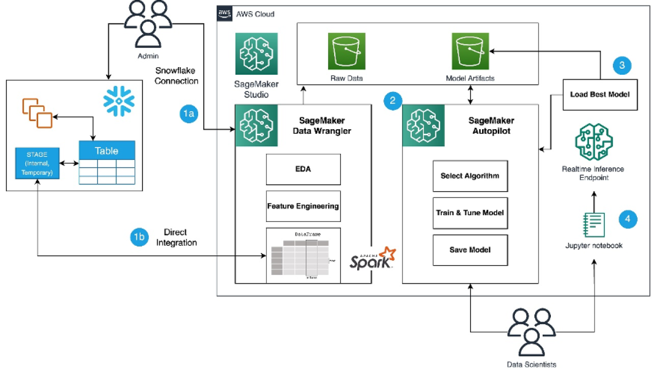
Refer to the diagram below for an overview of the low-code ML process with Snowflake, SageMaker Data Wrangler, and SageMaker Autopilot.

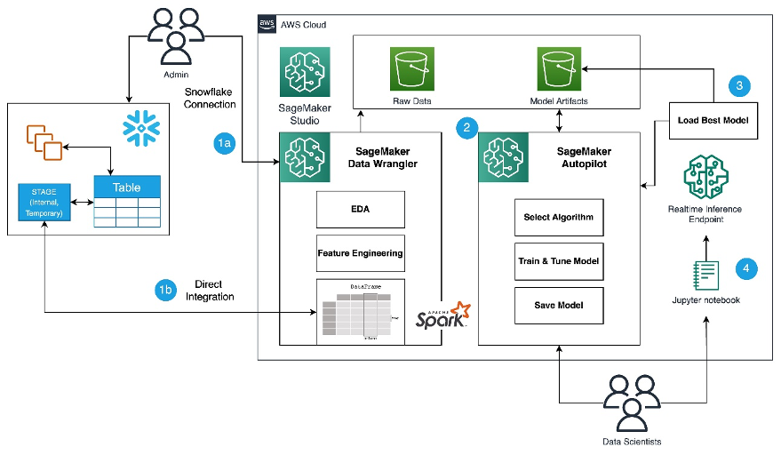
The workflow includes the following steps:

1. Navigate to SageMaker Data Wrangler for your data preparation and feature engineering tasks.
   • Set up the Snowflake connection with SageMaker Data Wrangler.
   • Explore your Snowflake tables in SageMaker Data Wrangler, create a ML dataset, and perform feature engineering.
2. Train and test the models using SageMaker Data Wrangler and SageMaker Autopilot.
3. Load the best model to a real-time inference endpoint for predictions.
4. Use a Python notebook to invoke the launched real-time inference endpoint.

Prerequisites

For this post, the administrator needs the following prerequisites:

• A Snowflake user with administrator permission to create a Snowflake virtual warehouse, user, and role, and grant access to this user to create a database. For more details on the administration setup, refer to Import data from Snowflake.
• An AWS account with admin access.
• A Snowflake Enterprise Account in your preferred AWS Region with ACCOUNTADMIN access.
• Optionally, if you’re using Snowflake OAuth access in SageMaker Data Wrangler, refer to Import data from Snowflake to set up an OAuth identity provider.
• Familiarity with Snowflake, basic SQL, the Snowsight UI, and Snowflake objects.

Data scientists should have the following prerequisites

• Access to Amazon SageMaker, an instance of Amazon SageMaker Studio, and a user for SageMaker Studio. For more information about prerequisites, see Get Started with Data Wrangler.
• Familiarity with AWS services, networking, and the AWS Management Console.
  Basic knowledge of Python, Jupyter notebooks, and ML.

Lastly, you should prepare your data for Snowflake

• We use credit card transaction data from Kaggle to build ML models for detecting fraudulent credit card transactions, so customers are not charged for items that they didn’t purchase. The dataset includes credit card transactions in September 2013 made by European cardholders.
• You should use the SnowSQL client and install it in your local machine, so you can use it to upload the dataset to a Snowflake table.

The following steps show how to prepare and load the dataset into the Snowflake database. This is a one-time setup.

Snowflake table and data preparation

Complete the following steps for this one-time setup:

1. First, as the administrator, create a Snowflake virtual warehouse, user, and role, and grant access to other users such as the data scientists to create a database and stage data for their ML use cases:

   -- Use the role SECURITYADMIN to create Role and User
   USE ROLE SECURITYADMIN;
   
   -- Create a new role 'ML Role'
   CREATE OR REPLACE ROLE ML_ROLE COMMENT='ML Role';
   GRANT ROLE ML_ROLE TO ROLE SYSADMIN;
   
   -- Create a new user and password and grant the role to the user
   CREATE OR REPLACE USER ML_USER PASSWORD='<REPLACE_PASSWORD>'
   DEFAULT_ROLE=ML_ROLE
   DEFAULT_WAREHOUSE=ML_WH
   DEFAULT_NAMESPACE=ML_WORKSHOP.PUBLIC
   COMMENT='ML User';
   GRANT ROLE ML_ROLE TO USER ML_USER;
   
   -- Grant privliges to role
   USE ROLE ACCOUNTADMIN;
   GRANT CREATE DATABASE ON ACCOUNT TO ROLE ML_ROLE;
   
   --Create Warehouse for AI/ML work
   USE ROLE SYSADMIN;
   
   CREATE OR REPLACE WAREHOUSE ML_WH
   WITH WAREHOUSE_SIZE = 'XSMALL' AUTO_SUSPEND = 120 AUTO_RESUME = true INITIALLY_SUSPENDED = TRUE;
   
   GRANT ALL ON WAREHOUSE ML_WH TO ROLE ML_ROLE;
   

2. As the data scientist, let’s now create a database and import the credit card transactions into the Snowflake database to access the data from SageMaker Data Wrangler. For illustration purposes, we create a Snowflake database named SF_FIN_TRANSACTION:

   -- Select the role and the warehouse
   USE ROLE ML_ROLE;
   USE WAREHOUSE ML_WH;
   
   -- Create the DB to import the financial transactions
   CREATE DATABASE IF NOT EXISTS sf_fin_transaction;
   
   -- Create CSV File Format
   create or replace file format my_csv_format
   type = csv
   field_delimiter = ','
   skip_header = 1
   null_if = ('NULL', 'null')
   empty_field_as_null = true
   compression = gzip;
   

3. Download the dataset CSV file to your local machine and create a stage to load the data into the database table. Update the file path to point to the downloaded dataset location before running the PUT command for importing the data to the created stage:

   -- Create a Snowflake named internal stage to store the transactions csv file
   CREATE OR REPLACE STAGE my_stage
   FILE_FORMAT = my_csv_format;
   
   -- Import the file in to the stage
   -- This command needs be run from SnowSQL client and not on WebUI
   PUT file:///Users/*******/Downloads/creditcard.csv @my_stage;
   
   -- Check whether the import was successful
   LIST @my_stage;
   

4. Create a table named credit_card_transactions:

   -- Create table and define the columns mapped to the csv transactions file
   create or replace table credit_card_transaction (
   Time integer,
   V1 float, V2 float, V3 float,
   V4 float, V5 float, V6 float,
   V7 float, V8 float, V9 float,
   V10 float,V11 float,V12 float,
   V13 float,V14 float,V15 float,
   V16 float,V17 float,V18 float,
   V19 float,V20 float,V21 float,
   V22 float,V23 float,V24 float,
   V25 float,V26 float,V27 float,
   V28 float,Amount float,
   Class varchar(5)
   );
   

5. Import the data into the created table from the stage:

   -- Import the transactions in to a new table named 'credit_card_transaction'
   copy into credit_card_transaction from @my_stage ON_ERROR = CONTINUE;
   
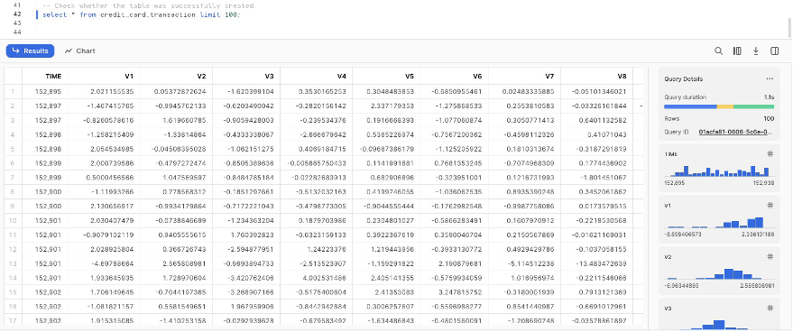
   -- Check whether the table was successfully created
   select * from credit_card_transaction limit 100;

Set up the SageMaker Data Wrangler and Snowflake connection

After we prepare the dataset to use with SageMaker Data Wrangler, let us create a new Snowflake connection in SageMaker Data Wrangler to connect to the sf_fin_transaction database in Snowflake and query the credit_card_transaction table:

1. Choose Snowflake on the SageMaker Data Wrangler Connection page.
2. Provide a name to identify your connection.
3. Select your authentication method to connect with the Snowflake database:
   • If using basic authentication, provide the user name and password shared by your Snowflake administrator. For this post, we use basic authentication to connect to Snowflake using the user credentials we created in the previous step.
   • If you are using OAuth, provide your identity provider credentials.

SageMaker Data Wrangler by default queries your data directly from Snowflake without creating any data copies in S3 buckets. SageMaker Data Wrangler’s new usability enhancement uses Apache Spark to integrate with Snowflake to prepare and seamlessly create a dataset for your ML journey.

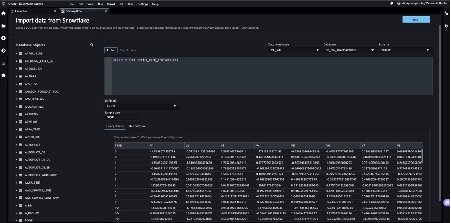
So far, we have created the database on Snowflake, imported the CSV file into the Snowflake table, created Snowflake credentials, and created a connector on SageMaker Data Wrangler to connect to Snowflake. To validate the configured Snowflake connection, run the following query on the created Snowflake table:

select * from credit_card_transaction;

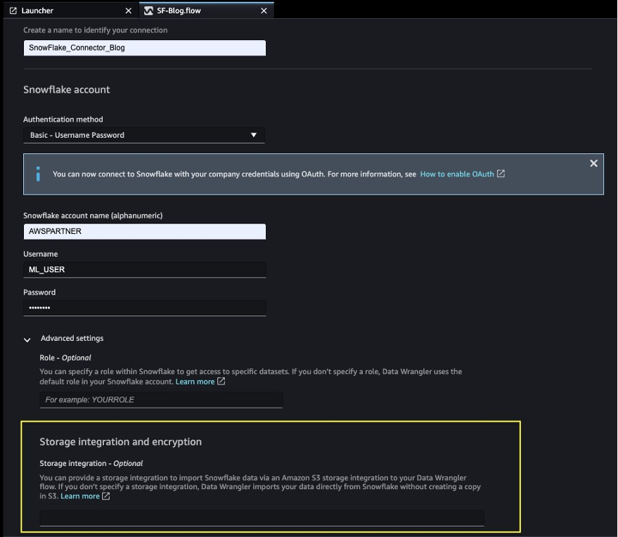
Note that the storage integration option that was required before is now optional in the advanced settings.

Explore Snowflake data

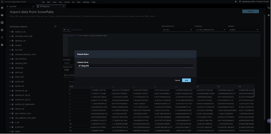
After you validate the query results, choose Import to save the query results as the dataset. We use this extracted dataset for exploratory data analysis and feature engineering.

You can choose to sample the data from Snowflake in the SageMaker Data Wrangler UI. Another option is to download complete data for your ML model training use cases using SageMaker Data Wrangler processing jobs.

Perform exploratory data analysis in SageMaker Data Wrangler

The data within Data Wrangler needs to be engineered before it can be trained. In this section, we demonstrate how to perform feature engineering on the data from Snowflake using SageMaker Data Wrangler’s built-in capabilities.

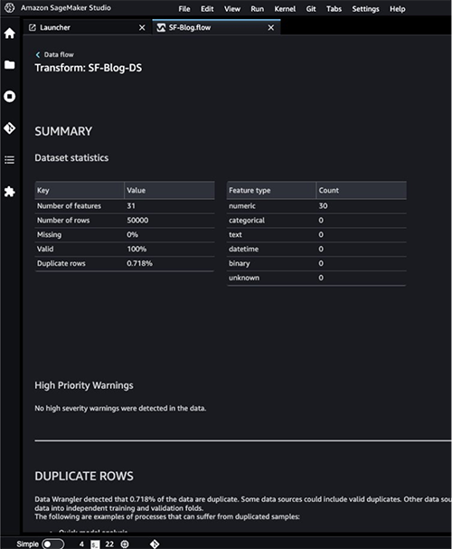
First, let’s use the Data Quality and Insights Report feature within SageMaker Data Wrangler to generate reports to automatically verify the data quality and detect abnormalities in the data from Snowflake.

You can use the report to help you clean and process your data. It gives you information such as the number of missing values and the number of outliers. If you have issues with your data, such as target leakage or imbalance, the insights report can bring those issues to your attention. To understand the report details, refer to Accelerate data preparation with data quality and insights in Amazon SageMaker Data Wrangler.

After you check out the data type matching applied by SageMaker Data Wrangler, complete the following steps:

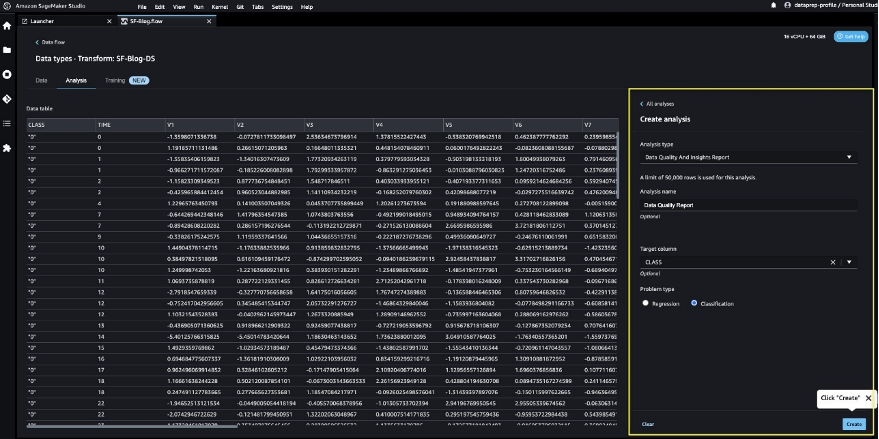
1. Choose the plus sign next to Data types and choose Add analysis.
   
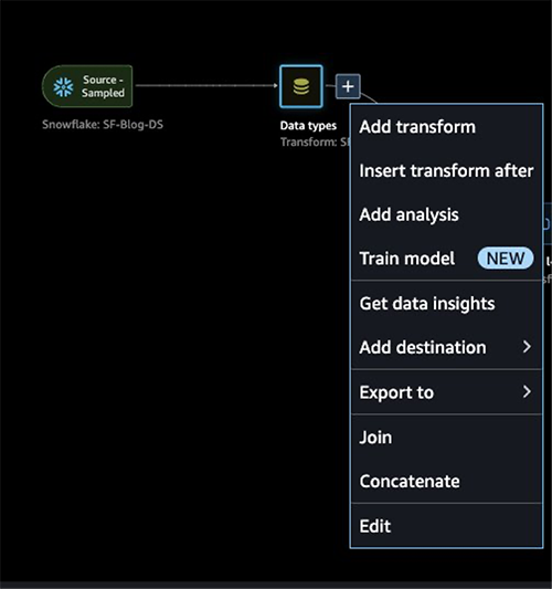
2. For Analysis type, choose Data Quality and Insights Report.
3. Choose Create.
   
4. Refer to the Data Quality and Insights Report details to check out high-priority warnings.

You can choose to resolve the warnings reported before proceeding with your ML journey.

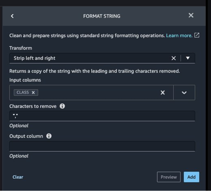
The target column Class to be predicted is classified as a string. First, let’s apply a transformation to remove the stale empty characters.

4. Choose Add step and choose Format string.
5. In the list of transforms, choose Strip left and right.
6. Enter the characters to remove and choose Add.

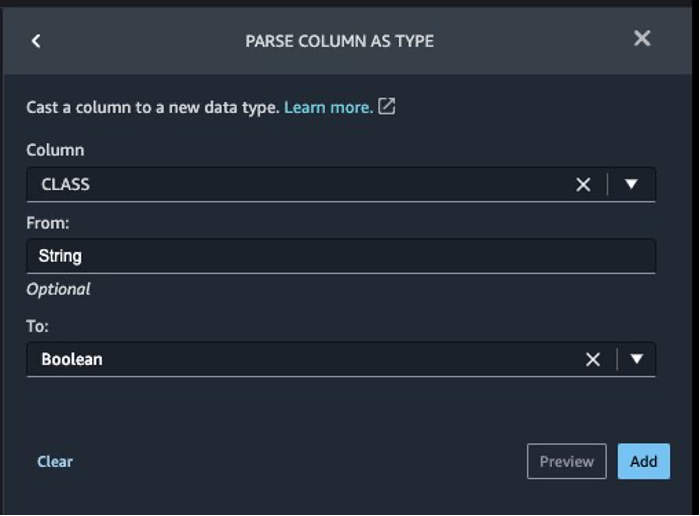
Next, we convert the target column Class from the string data type to Boolean because the transaction is either legitimate or fraudulent.

7. Choose Add step.
8. Choose Parse column as type.
9. For Column, choose Class.
10. For From, choose String.
11. For To, choose Boolean.
12. Choose Add.

After the target column transformation, we reduce the number of feature columns, because there are over 30 features in the original dataset. We use Principal Component Analysis (PCA) to reduce the dimensions based on feature importance. To understand more about PCA and dimensionality reduction, refer to Principal Component Analysis (PCA) Algorithm.

11. Choose Add step.
    
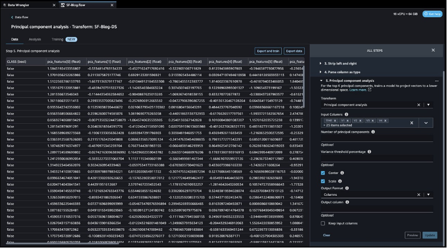
12. Choose Dimensionality Reduction.
    
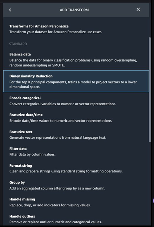
13. For Transform, choose Principal component analysis.
14. For Input columns, choose all the columns except the target column Class.
    
15. Choose the plus sign next to Data flow and choose Add analysis.
16. For Analysis type, choose Quick Model.
17. For Analysis name, enter a name.
18. For Label, choose Class.
    
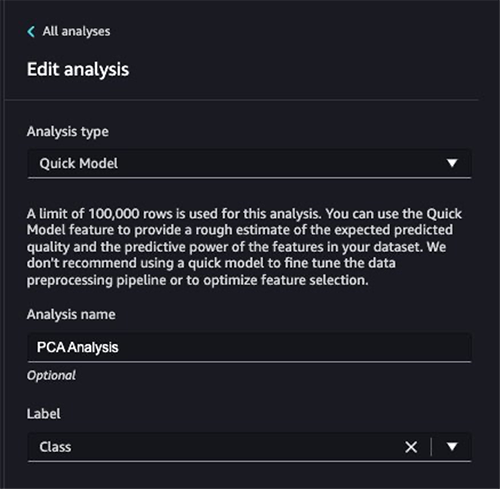
19. Choose Run.

Based on the PCA results, you can decide which features to use for building the model. In the following screenshot, the graph shows the features (or dimensions) ordered based on highest to lowest importance to predict the target class, which in this dataset is whether the transaction is fraudulent or valid.

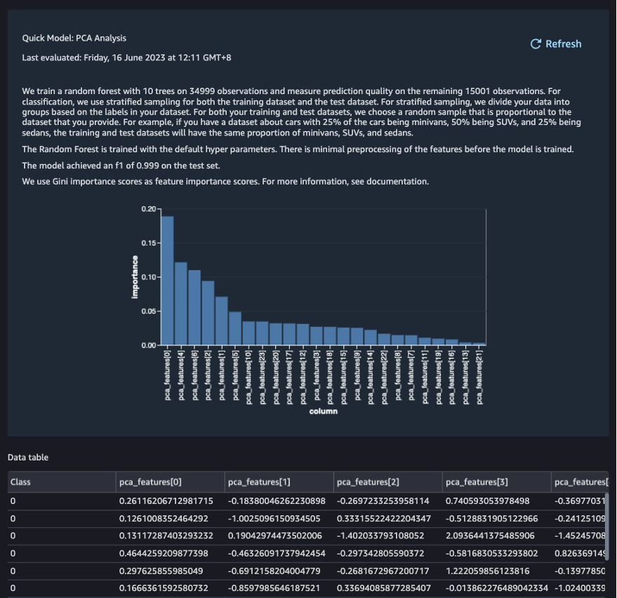
You can choose to reduce the number of features based on this analysis, but for this post, we leave the defaults as is.

This concludes our feature engineering process, although you may choose to run the quick model and create a Data Quality and Insights Report again to understand the data before performing further optimizations.

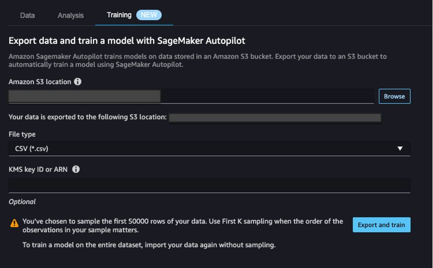
Export data and train the model

In the next step, we use SageMaker Autopilot to automatically build, train, and tune the best ML models based on your data. With SageMaker Autopilot, you still maintain full control and visibility of your data and model.

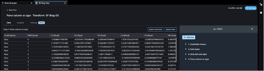
Now that we have completed the exploration and feature engineering, let’s train a model on the dataset and export the data to train the ML model using SageMaker Autopilot.

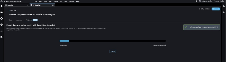
1. On the Training tab, choose Export and train.
   

We can monitor the export progress while we wait for it to complete.

Let’s configure SageMaker Autopilot to run an automated training job by specifying the target we want to predict and the type of problem. In this case, because we’re training the dataset to predict whether the transaction is fraudulent or valid, we use binary classification.

2. Enter a name for your experiment, provide the S3 location data, and choose Next: Target and features.
   
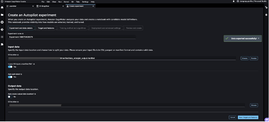
3. For Target, choose Class as the column to predict.
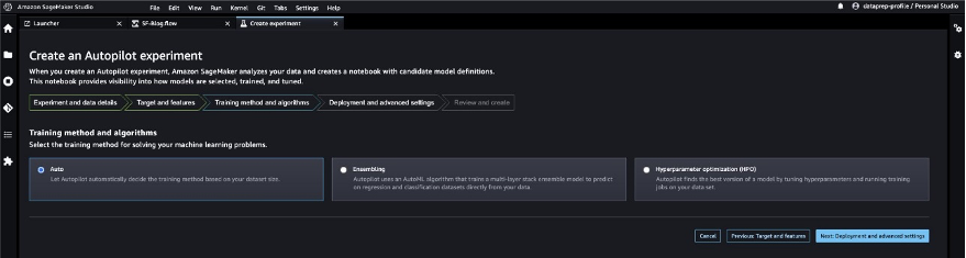
4. Choose Next: Training method.
   

Let’s allow SageMaker Autopilot to decide the training method based on the dataset.

5. For Training method and algorithms, select Auto.

To understand more about the training modes supported by SageMaker Autopilot, refer to Training modes and algorithm support.

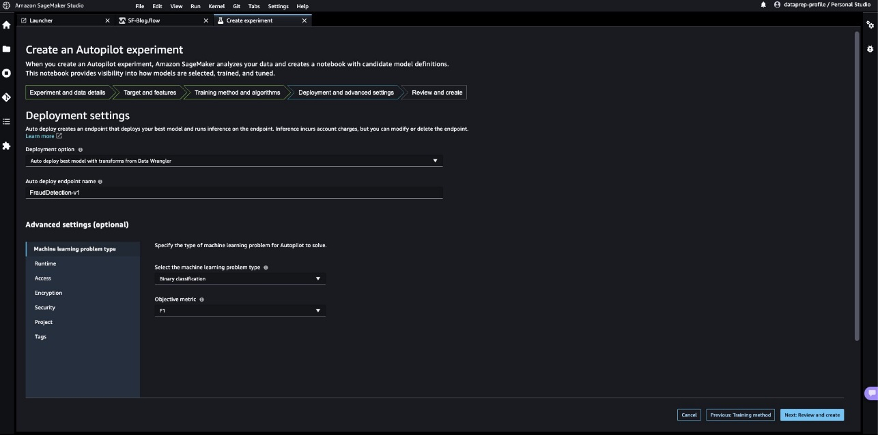
6. Choose Next: Deployment and advanced settings.
   
7. For Deployment option, choose Auto deploy the best model with transforms from Data Wrangler, which loads the best model for inference after the experimentation is complete.
8. Enter a name for your endpoint.
9. For Select the machine learning problem type, choose Binary classification.
10. For Objection metric, choose F1.
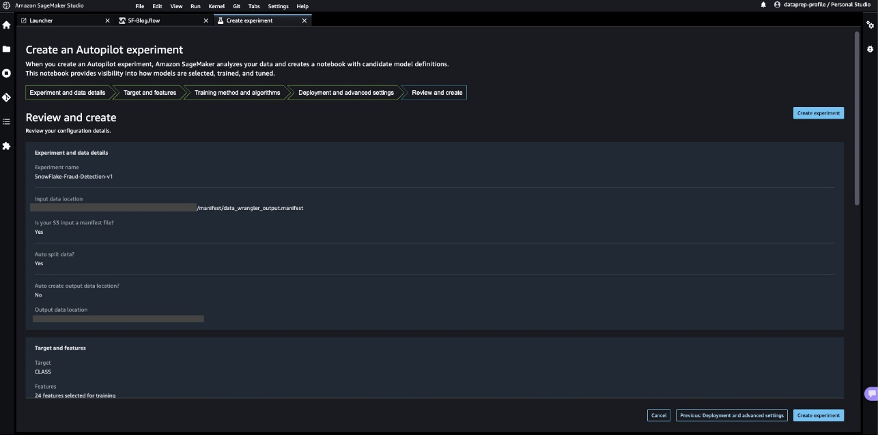
11. Choose Next: Review and create.
    
12. Choose Create experiment.

This starts an SageMaker Autopilot job that creates a set of training jobs that uses combinations of hyperparameters to optimize the objective metric.

Wait for SageMaker Autopilot to finish building the models and evaluation of the best ML model.

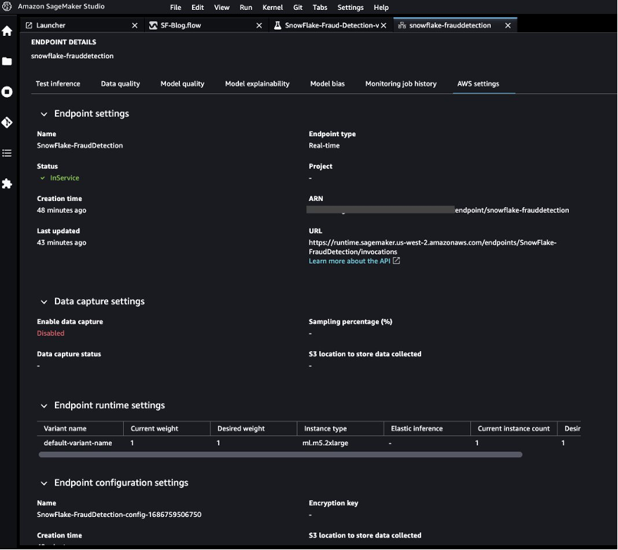
Launch a real-time inference endpoint to test the best model

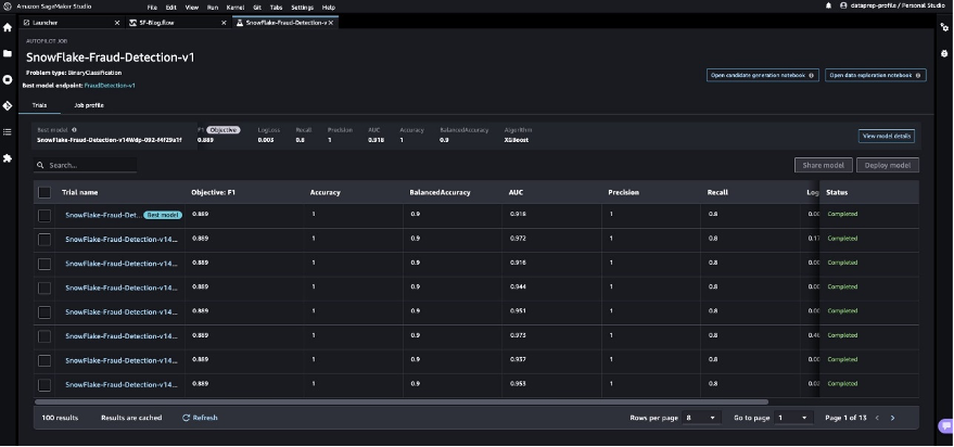
SageMaker Autopilot runs experiments to determine the best model that can classify credit card transactions as legitimate or fraudulent.

When SageMaker Autopilot completes the experiment, we can view the training results with the evaluation metrics and explore the best model from the SageMaker Autopilot job description page.

1. Select the best model and choose Deploy model.
   

We use a real-time inference endpoint to test the best model created through SageMaker Autopilot.

2. Select Make real-time predictions.
   

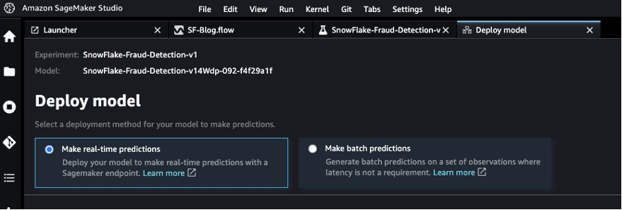
When the endpoint is available, we can pass the payload and get inference results.

Let’s launch a Python notebook to use the inference endpoint.

3. On the SageMaker Studio console, choose the folder icon in the navigation pane and choose Create notebook.
   
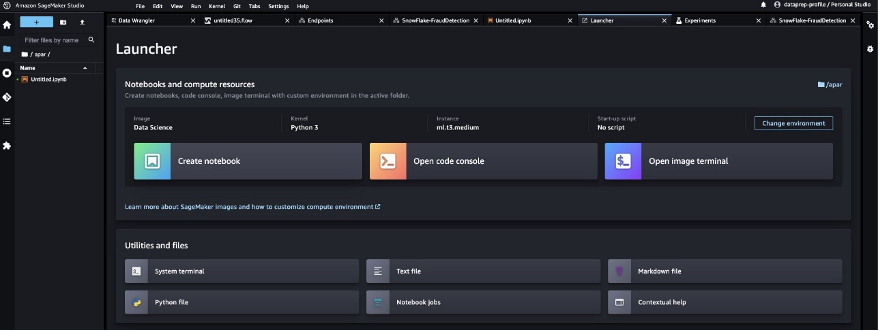
4. Use the following Python code to invoke the deployed real-time inference endpoint:

   # Library imports
   import os
   import io
   import boto3
   import json
   import csv
   
   #: Define the endpoint's name.
   ENDPOINT_NAME = 'SnowFlake-FraudDetection' # replace the endpoint name as per your config
   runtime = boto3.client('runtime.sagemaker')
   
   #: Define a test payload to send to your endpoint.
   payload = {
       "body": {
       "TIME": 152895,
       "V1": 2.021155535,
       "V2": 0.05372872624,
       "V3": -1.620399104,
       "V4": 0.3530165253,
       "V5": 0.3048483853,
       "V6": -0.6850955461,
       "V7": 0.02483335885,
       "V8": -0.05101346021,
       "V9": 0.3550896835,
       "V10": -0.1830053153,
       "V11": 1.148091498,
       "V12": 0.4283365505,
       "V13": -0.9347237892,
       "V14": -0.4615291327,
       "V15": -0.4124343184,
       "V16": 0.4993445934,
       "V17": 0.3411548305,
       "V18": 0.2343833846,
       "V19": 0.278223588,
       "V20": -0.2104513475,
       "V21": -0.3116427235,
       "V22": -0.8690778214,
       "V23": 0.3624146958,
       "V24": 0.6455923598,
       "V25": -0.3424913329,
       "V26": 0.1456884618,
       "V27": -0.07174890419,
       "V28": -0.040882382,
       "AMOUNT": 0.27
       }
   }
   
   #: Submit an API request and capture the response object.
   response = runtime.invoke_endpoint(
       EndpointName=ENDPOINT_NAME,
       ContentType='text/csv',
       Body=str(payload)
   )
   
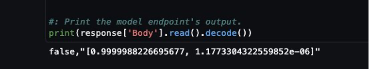
   #: Print the model endpoint's output.
   print(response['Body'].read().decode()) 
   

The output shows the result as false, which implies the sample feature data is not fraudulent.

Clean up

To make sure you don’t incur charges after completing this tutorial, shut down the SageMaker Data Wrangler application and shut down the notebook instance used to perform inference. You should also delete the inference endpoint you created using SageMaker Autopilot to prevent additional charges.

Conclusion

In this post, we demonstrated how to bring your data from Snowflake directly without creating any intermediate copies in the process. You can either sample or load your complete dataset to SageMaker Data Wrangler directly from Snowflake. You can then explore the data, clean the data, and perform featuring engineering using SageMaker Data Wrangler’s visual interface.

We also highlighted how you can easily train and tune a model with SageMaker Autopilot directly from the SageMaker Data Wrangler user interface. With SageMaker Data Wrangler and SageMaker Autopilot integration, we can quickly build a model after completing feature engineering, without writing any code. Then we referenced SageMaker Autopilot’s best model to run inferences using a real-time endpoint.

Try out the new Snowflake direct integration with SageMaker Data Wrangler today to easily build ML models with your data using SageMaker.

About the authors

Hariharan Suresh is a Senior Solutions Architect at AWS. He is passionate about databases, machine learning, and designing innovative solutions. Prior to joining AWS, Hariharan was a product architect, core banking implementation specialist, and developer, and worked with BFSI organizations for over 11 years. Outside of technology, he enjoys paragliding and cycling.

Aparajithan Vaidyanathan is a Principal Enterprise Solutions Architect at AWS. He supports enterprise customers migrate and modernize their workloads on AWS cloud. He is a Cloud Architect with 23+ years of experience designing and developing enterprise, large-scale and distributed software systems. He specializes in Machine Learning & Data Analytics with focus on Data and Feature Engineering domain. He is an aspiring marathon runner and his hobbies include hiking, bike riding and spending time with his wife and two boys.

Tim Song is a Software Development Engineer at AWS SageMaker, with 10+ years of experience as software developer, consultant and tech leader he has demonstrated ability to deliver scalable and reliable products and solve complex problems. In his spare time, he enjoys the nature, outdoor running, hiking and etc.

Bosco Albuquerque is a Sr. Partner Solutions Architect at AWS and has over 20 years of experience in working with database and analytics products from enterprise database vendors and cloud providers. He has helped large technology companies design data analytics solutions and has led engineering teams in designing and implementing data analytics platforms and data products.

Read More

For data scientists, moving machine learning (ML) models from proof of concept to production often presents a significant challenge. One of the main challenges can be deploying a well-performing, locally trained model to the cloud for inference and use in other applications. It can be cumbersome to manage the process, but with the right tool, you can significantly reduce the required effort.

Amazon SageMaker inference, which was made generally available in April 2022, makes it easy for you to deploy ML models into production to make predictions at scale, providing a broad selection of ML infrastructure and model deployment options to help meet all kinds of ML inference needs. You can use SageMaker Serverless Inference endpoints for workloads that have idle periods between traffic spurts and can tolerate cold starts. The endpoints scale out automatically based on traffic and take away the undifferentiated heavy lifting of selecting and managing servers. Additionally, you can use AWS Lambda directly to expose your models and deploy your ML applications using your preferred open-source framework, which can prove to be more flexible and cost-effective.

FastAPI is a modern, high-performance web framework for building APIs with Python. It stands out when it comes to developing serverless applications with RESTful microservices and use cases requiring ML inference at scale across multiple industries. Its ease and built-in functionalities like the automatic API documentation make it a popular choice amongst ML engineers to deploy high-performance inference APIs. You can define and organize your routes using out-of-the-box functionalities from FastAPI to scale out and handle growing business logic as needed, test locally and host it on Lambda, then expose it through a single API gateway, which allows you to bring an open-source web framework to Lambda without any heavy lifting or refactoring your codes.

This post shows you how to easily deploy and run serverless ML inference by exposing your ML model as an endpoint using FastAPI, Docker, Lambda, and Amazon API Gateway. We also show you how to automate the deployment using the AWS Cloud Development Kit (AWS CDK).

Solution overview

The following diagram shows the architecture of the solution we deploy in this post.

Prerequisites

You must have the following prerequisites:

• Python3 installed, along with virtualenv for creating and managing virtual environments in Python
• aws-cdk v2 installed on your system in order to be able to use the AWS CDK CLI
• Docker installed and running on your local machine

Test if all the necessary software is installed:

1. The AWS Command Line Interface (AWS CLI) is needed. Log in to your account and choose the Region where you want to deploy the solution.
2. Use the following code to check your Python version:

   python3 --version

3. Check if virtualenv is installed for creating and managing virtual environments in Python. Strictly speaking, this is not a hard requirement, but it will make your life easier and helps follow along with this post more easily. Use the following code:

   python3 -m virtualenv --version

4. Check if cdk is installed. This will be used to deploy our solution.

   cdk --version

5. Check if Docker is installed. Our solution will make your model accessible through a Docker image to Lambda. To build this image locally, we need Docker.

   docker --version

6. Make sure Docker is up and running with the following code:

   docker ps

How to structure your FastAPI project using AWS CDK

We use the following directory structure for our project (ignoring some boilerplate AWS CDK code that is immaterial in the context of this post):

```

fastapi_model_serving
│
└───.venv
│
└───fastapi_model_serving
│   │   __init__.py
│   │   fastapi_model_serving_stack.py
│   │
│   └───model_endpoint
│       └───docker
│       │      Dockerfile
│       │      serving_api.tar.gz
│
│
│       └───runtime
│            └───serving_api
│                    requirements.txt
│                    serving_api.py
│                └───custom_lambda_utils
│                     └───model_artifacts
│                            ...
│                     └───scripts
│                            inference.py
│
└───templates
│   └───api
│   │     api.py
│   └───dummy
│         dummy.py
│
│ app.py
│   cdk.json
│   README.md
│   requirements.txt
│   init-lambda-code.sh

```

The directory follows the recommended structure of AWS CDK projects for Python.

The most important part of this repository is the fastapi_model_serving directory. It contains the code that will define the AWS CDK stack and the resources that are going to be used for model serving.

The fastapi_model_serving directory contains the model_endpoint subdirectory, which contains all the assets necessary that make up our serverless endpoint, namely the Dockerfile to build the Docker image that Lambda will use, the Lambda function code that uses FastAPI to handle inference requests and route them to the correct endpoint, and the model artifacts of the model that we want to deploy. model_endpoint also contains the following:

• Docker– This subdirectory contains the following:
• Dockerfile – This is used to build the image for the Lambda function with all the artifacts (Lambda function code, model artifacts, and so on) in the right place so that they can be used without issues.
• serving.api.tar.gz – This is a tarball that contains all the assets from the runtime folder that are necessary for building the Docker image. We discuss how to create the .tar.gz file later in this post.
• runtime– This subdirectory contains the following:
• serving_api – The code for the Lambda function and its dependencies specified in the requirements.txt file.
• custom_lambda_utils – This includes an inference script that loads the necessary model artifacts so that the model can be passed to the serving_api that will then expose it as an endpoint.

Additionally, we have the template directory, which provides a template of folder structures and files where you can define your customized codes and APIs following the sample we went through earlier. The template directory contains dummy code that you can use to create new Lambda functions:

• dummy – Contains the code that implements the structure of an ordinary Lambda function using the Python runtime
• api – Contains the code that implements a Lambda function that wraps a FastAPI endpoint around an existing API gateway

Deploy the solution

By default, the code is deployed inside the eu-west-1 region. If you want to change the Region, you can change the DEPLOYMENT_REGION context variable in the cdk.json file.

Keep in mind, however, that the solution tries to deploy a Lambda function on top of the arm64 architecture, and that this feature might not be available in all Regions. In this case, you need to change the architecture parameter in the fastapi_model_serving_stack.py file, as well as the first line of the Dockerfile inside the Docker directory, to host this solution on the x86 architecture.

To deploy the solution, complete the following steps:

1. Run the following command to clone the GitHub repository: git clone https://github.com/aws-samples/lambda-serverless-inference-fastapiBecause we want to showcase that the solution can work with model artifacts that you train locally, we contain a sample model artifact of a pretrained DistilBERT model on the Hugging Face model hub for a question answering task in the serving_api.tar.gz file. The download time can take around 3–5 minutes. Now, let’s set up the environment.
2. Download the pretrained model that will be deployed from the Hugging Face model hub into the ./model_endpoint/runtime/serving_api/custom_lambda_utils/model_artifacts directory. It also creates a virtual environment and installs all dependencies that are needed. You only need to run this command once: make prep. This command can take around 5 minutes (depending on your internet bandwidth) because it needs to download the model artifacts.
3. Package the model artifacts inside a .tar.gz archive that will be used inside the Docker image that is built in the AWS CDK stack. You need to run this code whenever you make changes to the model artifacts or the API itself to always have the most up-to-date version of your serving endpoint packaged: make package_model. The artifacts are all in place. Now we can deploy the AWS CDK stack to your AWS account.
4. Run cdk bootstrap if it’s your first time deploying an AWS CDK app into an environment (account + Region combination):

   make cdk_bootstrap

   This stack includes resources that are needed for the toolkit’s operation. For example, the stack includes an Amazon Simple Storage Service (Amazon S3) bucket that is used to store templates and assets during the deployment process.

   Because we’re building Docker images locally in this AWS CDK deployment, we need to ensure that the Docker daemon is running before we can deploy this stack via the AWS CDK CLI.

5. To check whether or not the Docker daemon is running on your system, use the following command:

   docker ps

   If you don’t get an error message, you should be ready to deploy the solution.

6. Deploy the solution with the following command:

   make deploy

   This step can take around 5–10 minutes due to building and pushing the Docker image.

Troubleshooting

If you’re a Mac user, you may encounter an error when logging into Amazon Elastic Container Registry (Amazon ECR) with the Docker login, such as Error saving credentials ... not implemented. For example:

exited with error code 1: Error saving credentials: error storing credentials - err: exit status 1,...dial unix backend.sock: connect: connection refused

Before you can use Lambda on top of Docker containers inside the AWS CDK, you may need to change the ~/docker/config.json file. More specifically, you might have to change the credsStore parameter in ~/.docker/config.json to osxkeychain. That solves Amazon ECR login issues on a Mac.

Run real-time inference

After your AWS CloudFormation stack is deployed successfully, go to the Outputs tab for your stack on the AWS CloudFormation console and open the endpoint URL. Now our model is accessible via the endpoint URL and we’re ready to run real-time inference.

Navigate to the URL to see if you can see “hello world” message and add /docs to the address to see if you can see the interactive swagger UI page successfully. There might be some cold start time, so you may need to wait or refresh a few times.

After you log in to the landing page of the FastAPI swagger UI page, you can run via the root / or via /question.

From /, you could run the API and get the “hello world” message.

From /question, you could run the API and run ML inference on the model we deployed for a question answering case. For example, we use the question is What is the color of my car now? and the context is My car used to be blue but I painted red.

When you choose Execute, based on the given context, the model will answer the question with a response, as shown in the following screenshot.

In the response body, you can see the answer with the confidence score from the model. You could also experiment with other examples or embed the API in your existing application.

Alternatively, you can run the inference via code. Here is one example written in Python, using the requests library:

import requests

url = "https://<YOUR_API_GATEWAY_ENDPOINT_ID>.execute-api.<YOUR_ENDPOINT_REGION>.amazonaws.com/prod/question?question="What is the color of my car now?"&context="My car used to be blue but I painted red""

response = requests.request("GET", url, headers=headers, data=payload)

print(response.text)

The code outputs a string similar to the following:

'{"score":0.6947233080863953,"start":38,"end":41,"answer":"red"}'

If you are interested in knowing more about deploying Generative AI and large language models on AWS, check out here:

• Deploy Serverless Generative AI on AWS Lambda with OpenLLaMa
• Deploy large language models on AWS Inferentia2 using large model inference containers

Clean up

Inside the root directory of your repository, run the following code to clean up your resources:

make destroy

Conclusion

In this post, we introduced how you can use Lambda to deploy your trained ML model using your preferred web application framework, such as FastAPI. We provided a detailed code repository that you can deploy, and you retain the flexibility of switching to whichever trained model artifacts you process. The performance can depend on how you implement and deploy the model.

You are welcome to try it out yourself, and we’re excited to hear your feedback!

About the Authors

Tingyi Li is an Enterprise Solutions Architect from AWS based out in Stockholm, Sweden supporting the Nordics customers. She enjoys helping customers with the architecture, design, and development of cloud-optimized infrastructure solutions. She is specialized in AI and Machine Learning and is interested in empowering customers with intelligence in their AI/ML applications. In her spare time, she is also a part-time illustrator who writes novels and plays the piano.

Demir Catovic is a Machine Learning Engineer from AWS based in Zurich, Switzerland. He engages with customers and helps them implement scalable and fully-functional ML applications. He is passionate about building and productionizing machine learning applications for customers and is always keen to explore around new trends and cutting-edge technologies in the AI/ML world.

Read More