Field to Fork: Startup Serves Food Industry an AI Smorgasbord

Field to Fork: Startup Serves Food Industry an AI Smorgasbord

It worked like magic. Computer vision algorithms running in a data center saw that a disease was about to infect a distant wheat field in India.

Sixteen days later, workers in the field found the first evidence of the outbreak.

It was the kind of wizardry people like Vinay Indraganti call digital transformation. He’s practiced it for 25 years, the last dozen of them at companies like Ingredion, a Fortune 500 food-ingredient producer.

The India project was the first big test of AGRi360 — a product suite for sustainable agriculture powered by NVIDIA Metropolis — from the startup that Indraganti co-founded, Blu Cocoon Digital.

Mobile App Taps Cloud Smarts

The pilot was both simple and effective.

Farm workers took pictures of the plants, time-stamped and geotagged by a mobile app. They sent them to the Microsoft Azure cloud, where Blu Cocoon’s custom models found patterns that enabled their uncanny prediction.

Thanks to his background in the industry, Indraganti knows the value of such timely intelligence. It can help farmers and their entire food chain of vendors reap a bumper harvest.

“It’s a vast area, that’s why we’ve made ‘AI for food’ our mantra at Blu Cocoon,” he said in an interview from the suburban Chicago office of the company headquartered in Kolkata.

A Third Eye on the Field

AGRi360 acts “like a third eye in the field,” said Pinaki Bhattacharya, a microbiologist who heads R&D at Blu Cocoon Digital.

Screen shot of the Agri360 AI-powered farming app
AGRi360 puts a dashboard of AI-powered tool in farmers’ hands.

In the pilot, it gave farmers an early warning to apply a small amount of pesticide to arrest the disease. An agrochemical company got a heads up about conditions in the area, helping it manage its supply chain.

In the future, food producers that buy the crops will get key details about their microbiology. That helps in planning exactly how and when to process the crops into products to meet the regulatory requirements where they’ll be sold.

“AGRi360 captures all these insights thanks to AI fed by pictures from farmworkers taken while they’re doing their regular jobs,” Bhattacharya said.

Evaluating Seeds and Soils

The AI models got their start in research using computer vision to quickly assess soil conditions and the quality of seeds.

Those skills are now part of the AGRi360 product portfolio along with products that monitor plant health and best practices in farming. Today, AGRi360 is in use in two countries, improving the quantity and quality of crop yields.

One customer reports it’s on track to source 100% of its products sustainably by 2025. Another saw revenues for an insecticide rise, thanks to the service.

“Our sales of Cartap 50sp grew 70% in six months thanks to AGRi360’s ability to identify emerging crop infections early,” said Vandan Churiwal, a director at Krishi Rayasan, a leading agrochemical supplier based in Kolkata.

“As a result, we’re expanding our license with Blu Cocoon to bring AI-powered insights into every area of our business,” he said.

Faster Training and Inference

Initially, the startup used CPUs to train and run its AI models. Now it exclusively uses NVIDIA GPUs and the Metropolis framework for computer vision.

“It used to take us two months to train a single AI model on CPUs,” said Indraganti. “Now, with NVIDIA A10 Tensor Core GPUs, all four models in AGRi360 can be trained in a few hours — that’s a game changer.”

The time savings add up quickly because the models need to be retrained for new crops, variants and soil types.

GPUs reduced the time to complete inference jobs, too. Predictions that require 15-20 minutes on CPUs get generated in 2-3 seconds on NVIDIA T4 Tensor Core GPUs. The speed also enables Blu Cocoon to test its models on large and growing datasets.

From Shipyards to Snack Bars

Looking ahead, Blu Cocoon is extending its work in the food supply chain into managing containers in shipyards. It’s already testing computer vision models for a customer in India.

“We’ve figured out a way to optimize movement of containers, reducing their time in the yard and minimizing touch points to save time and money,” said Indraganti.

The startup is even helping food producers create recipes with AI. It’s already cooked up a gluten-free muffin for one packaged-foods client with plant-based cheeses, shakes and snack bars next on the menu.

One customer reports the AI-powered system helped reduce the time to create a new recipe by 80%.

“We named the company Blu Cocoon Digital because we look beyond the horizon and across the ocean for ways to nurture our customers’ aspirations with digital technology — and it all runs on the NVIDIA platform and Microsoft Azure,” he said.

Read about Monarch Tractor to learn other ways AI is advancing agriculture.

Read More

Matice Founder and Harvard Professor, Jessica Whited on Harnessing Regenerative Species – and AI – for Medical Breakthroughs

Matice Founder and Harvard Professor, Jessica Whited on Harnessing Regenerative Species – and AI – for Medical Breakthroughs

Scientists at Matice Biosciences are using AI to study the regeneration of tissues in animals known as super-regenerators, such as salamanders and planarians.

The goal of the research is to develop new treatments that will help humans heal from injuries without scarring.

On the latest episode of NVIDIA’s AI Podcast, host Noah Kravtiz spoke with Jessica Whited, a regenerative biologist at Harvard University and co-founder of Matice Biosciences.

Whited was inspired to start the company after her son suffered a severe injury while riding his bike.

She realized that while her work had been dedicated ultimately to limb regeneration, the short-term byproduct of it was a wealth of information that could be used to harness this regenerative science into topical treatments that can be put in the hands of everyday people, like her son and many others, who would no longer have to live with the physical scars of their trauma.

This led her to investigate the connection between regeneration and scarring.

Whited and her team are using AI to analyze the molecular and cellular mechanisms that control regeneration and scarring in super-regenerators.

They believe that by understanding these mechanisms, they can develop new treatments to help humans heal from injuries without scarring.

To learn more about Matice, please visit www.maticebio.com or follow along on Instagram, Twitter, Facebook and LinkedIn.

You Might Also Like

Jules Anh Tuan Nguyen Explains How AI Lets Amputee Control Prosthetic Hand, Video Games

A postdoctoral researcher at the University of Minnesota discusses his efforts to allow amputees to control their prosthetic limb — right down to the finger motions — with their minds.

Overjet’s Ai Wardah Inam on Bringing AI to Dentistry

Overjet, a member of NVIDIA Inception, is moving fast to bring AI to dentists’ offices. Dr. Wardah Inam, CEO of the company, discusses using AI to improve patient care.

Immunai CTO and Co-Founder Luis Voloch on Using Deep Learning to Develop New Drugs

Luis Voloch, co-founder and chief technology officer of Immunai, talks about tackling the challenges of the immune system with a machine learning and data science mindset.

Subscribe to the AI Podcast: Now Available on Amazon Music

The AI Podcast is now available through Amazon Music.

In addition, get the AI Podcast through iTunes, Google Podcasts, Google Play, Castbox, DoggCatcher, Overcast, PlayerFM, Pocket Casts, Podbay, PodBean, PodCruncher, PodKicker, Soundcloud, Spotify, Stitcher and TuneIn.

Make the AI Podcast better. Have a few minutes to spare? Fill out this listener survey.

Featured Image Credit: Matice Biosciences

Read More

Figure 1: LLaMA Inference Performance on TPU v4 hardware

The Path to Achieve Ultra-Low Inference Latency With LLaMA 65B

Background & State of the Art

In the natural language processing (NLP) space, language models are designed to generate a token (e.g. word) using a sequence of past input tokens. Large Language Models (LLMs) are the latest deep learning innovation in this space built to generate text in a human-like fashion. These models generally use transformers to improve their attention over a large sequence of input tokens.

LLaMA, open sourced by Meta AI, is a powerful foundation LLM trained on over 1T tokens. LLaMA is competitive with many best-in-class models such as GPT-3, Chinchilla, PaLM. LLaMA (13B) outperforms GPT-3 (175B) highlighting its ability to extract more compute from each model parameter.

In this blog post, we use LLaMA as an example model to demonstrate the capabilities of PyTorch/XLA for LLM inference. We discuss how the computation techniques and optimizations discussed here improve inference latency by 6.4x on 65B parameter LLaMA models powered by Google Cloud TPU v4 (v4-16).

Model Overview

We demonstrate the performance capabilities of PyTorch/XLA on LLaMA, the latest LLM from Meta. We showcase performance optimizations on a series of common LLaMA configurations. Notice the 175B parameter model configuration is absent in the public domain. For the 175B parameter model mentioned below, we apply OPT 175B model configuration to the LLaMA code base. Unless stated otherwise, in all configurations, we use max_seq_len=256 and dtype=bfloat16 for weights and activations.

Table 1: Model Configurations Explored in this article

LLaMA Model Hyper Parameters
# Parameters Dimensions N Heads N Layers Max Seq Len
7B 4,096 32 32 256
33B 6,656 52 60 256
65B 8,192 64 80 256
175B 12,288 96 96 256

Performance Challenges of LLMs

LLMs have a few properties that make them challenging for compiler optimizations. (a) LLMs use autoregressive decoding to generate the next token baked on the previous ones; this means prompt tensors and coaches have a dynamic shape. (b) LLMs must work with variable input prompt lengths without triggering recompilation due to input tensor shape changes; input tensors must be properly bucketized and padded to avoid recompilation. (c) LLMs often require more memory than a single TPU (or GPU) device can support. A model-sharding scheme is required to fit the model across a distributed compute architecture. For instance, a LLaMA model with 65B parameters can fit on a v4-16 Cloud TPU, which is comparable to 8 A100 GPUs. (d) running LLMs in production can be expensive; one way to improve performance per total cost of ownership (Perf/TCO) is via quantization; quantization can potentially reduce hardware requirements.

Inference Tech Stack in PyTorch/XLA

Our goal is to offer the AI community a high performance inference stack. PyTorch/XLA integrates with TorchDynamo, PjRt, OpenXLA, and various model parallelism schemes. TorchDynamo eliminates tracing overhead at runtime, PjRt enables efficient host-device communication; PyTorch/XLA traceable collectives enable model and data parallelism on LLaMA via TorchDynamo. To try our results, please use our custom torch, torch-xla wheels to reproduce our LLaMA inference solution. PyTorch/XLA 2.1 will support the features discussed in this post by default.

Parallel Computing

FairScale Sharding

LLaMA uses FairScale model sharding API (fairscale.nn.model_parallel.layers). We built an equivalent representation of this API using PyTorch/XLA communication collective (CC) ops such as all-reduce to communicate program state (e.g. activations) between accelerators. TorchDynamo does not fully support capturing CC ops currently (a.k.a. traceable collectives). Without this support, a TorchDynamo FX graph would be cut at every device communication, meaning at every model layer. Graph cuts lead to performance loss as the underlying XLA compiler loses full graph optimization opportunities. To resolve this, we offer PyTorch/XLA traceable collectives by integrating the dispatcher collectives into our existing CC APIs. The difference is we don’t need to insert c10d.wait() ops after collectives, given the lazy execution nature of PyTorch/XLA. With support for traceable collectives, PyTorch/XLA allows singular FX graph generation in TorchDynamo.

Autoregressive Decoding on PyTorch/XLA

LLMs need autoregressive decoding to feed the previous word as a prompt to predict the next token. Autoregressive decoding leads to unbounded dynamic shape problems, which in turn causes recompilation of every prompt. We optimized the LLaMA autoregressive decoder to operate with fixed shapes that in-place updates the KV-cache, output sequences, and attention masks during every token generation. With a combination of padding, masking, and index ops, we avoided excessive graph recompilation, thereby achieving efficient autoregressive decoding.

KV-Cache Optimization

LLaMA implements autoregressive decoding with KV-cache. For every generated token, the KV-cache stores the attention key/value activations of each Transformer layer. Thus, upon decoding a new token, the key/values of prior tokens no longer need recomputation.

In LLaMA, the KV-cache tensor slices are updated in-place; this leads to recompilation events every time a token is generated. To address this issue, we use index tensors and tensor.index_copy() ops to replace the in-place slice updates. Attention masks and output sequences also benefit from the same optimization.

Input Prompt Optimization

Variable length input prompts are common in LLM applications. This property causes input tensor shape dynamism and in turn recompilation events. When processing a prompt to fill the KV-cache, we either (a) process the input prompt token-by-token, or (b) process the whole prompt in one iteration. The pros and cons of each method are:

  1. Pre-compile 1 graph and process a prompt token-by-token
    • Practical: 1 graph is compiled during warm-up
    • Slow: O(L) to process an input prompt length L – a disadvantage for long prompts
  2. Pre-compile all graphs with input lengths ranging from 1 to max_seq_len (e.g. 2,048)
    • Impractical: pre-compile and cache max_seq_len graphs during warm-up time
    • Fast: 1 graph execution to process the full prompt

We introduce prompt length bucketization, an optimization to strike a balance between the two alternatives. We define a set of ascending bucket sizes, (b0,b1,b2,…,bB-1), and then pre-compile program graphs with input sizes according to these bucket values, (G0,G1,G2,…,GB-1); B is the number of buckets. For a given input prompt, we round up the prompt length to the closest bucket value bn, pad the sequence, and use Gn to process the prompt in one iteration. The computation on the padding tokens is discarded. For prompts larger than the largest bucket size, we process them section-by-section.

The optimal bucket sizes should be determined by prompt length distribution in a target application. Here, we adopt bucket lengths: 128, 256, 384, 512. Any input prompt with up to 2,047 tokens requires up to 4 graph executions. For example, a 1,500 input prompt with generation length of 256 requires 260 graph executions – 4 to process the input, and 256 to generate the output.

Quantization

Quantization reduces the number of bits necessary to represent a value; it reduces the bandwidth to communicate data across multiple accelerator nodes (via collectives) and lowers the hardware requirements to serve a specific model size.

Normally, with BF16 weights, a 175B parameter model would consume about 351GB of memory, and therefore require a v4-32 instance to accommodate the model. By quantizing the weights to INT8, we reduced the model size by roughly 50%, allowing it to run on a smaller v4-16 instance. Because LLaMA shards model activations, quantization offers negligible communication gain.

In our experiments, we quantized the linear layer. Since LLaMA model checkpoints are unavailable publicly, and our goal is to evaluate performance, the quantized model is initialized with random weights.Recent literature such as AWQ and Integer or Floating Point? offer insights into performance properties of LLaMA under various low-bit quantization schemes.

Effect of Batch Size on Quantization Performance

TPU v4 is programmed to run matmul on the Matrix Multiply Unit (MXU) when the model batch size (BS) > 1. For BS = 1, matmul runs on the Vector Processor Unit (VPU). Since MXU is more efficient than VPU, INT8 quantization gains performance at BS>1. See Performance Analysis section for details.

Op Support

Occasionally, new models introduce new mathematical operations that require PyTorch/XLA to extend its supported op set for compilation. For LLaMA, we supported: multinomial.

Methodology

LLaMA works on PyTorch/XLA out of the box on LazyTensorCore. We use this configuration as a baseline for our follow up analysis. All experiments assume 256-long input prompts. In the absence of a publicly available model checkpoint, we used random tensor initialization for this inference stack optimization effort. A model checkpoint is not expected to change latency results discussed here.

Model Sizing

Assuming N is the number of parameters, dimensions is the hidden size, n_layers is the number of layers, n_heads is the number of attention heads, the equation below can be used to approximate the model size. See the Model Overview section for details.

N = (dimensions)^2 * n_layers * 12

n_heads doesn’t affect N, but the following equation holds for the open sourced model configs.

dim = 128 * n_heads

Cache Sizing

Both model parameters and the cache layers in the Attention block contribute to memory consumption. Since the default LLaMA model uses BF16 weights, the memory consumption calculation in this section is based on BF16 weights.

The size of the cache layer is calculated by cache_size = max_batch_size * max_seq_len * dimensions. max_batch_size = 1 and max_seq_len = 256 are used as an example configuration in the following calculations. There are 2 cache layers in each Attention block. So, the total LLaMA cache size (in Bytes) is total_cache_size = n_layers * 2 * cache_size * (2 bytes).

TPU v4 Hardware Sizing

Each TPU v4 chip has 32GB of available High-Bandwidth Memory (HBM). Table 2 has the details on memory consumption and the number of required TPU chips to hold a LLaMA model.

Table 2: LLaMA TPU v4 HBM requirements (i.e. TPU v4 chip requirements)

# Parameters Parameter (MB) Cache (MB) Total (GB) Min # of TPU v4 Chips
7B 14,000 134 14.128 1
33B 66,000 408 66.41 3
65B 130,000 671 130.67 5
175B 350,000 1,208 351.21 11

Metrics

Below are useful metrics to measure inference speed. Assuming T is the total time, B is the batch size, L is the decoded sequence length.

Latency Definition

Latency is the time it takes to get the decoded result at target length L, regardless of the batch size B. Latency represents how long the user should wait to get the response from the generation model.

Latency = T (s)

Per-token latency

One step of autoregressive decoding generates a token for each sample in the batch. Per-token latency is the average time for that one step.

Per-token latency = T / L (s/token)

Throughput

Throughput measures how many tokens are generated per unit time. While it’s not a useful metric for evaluating online serving it is useful to measure the speed of batch processing.

Throughput = B * L / T (tokens/s)

To minimize confusion and misinterpretation, it’s better to avoid metrics like T / (B * L), which mixes latency and throughput.

Results

Figure 1 shows latency / token results for LLaMA 7B to 175B models. In each case, the model is run on a range of TPU v4 configurations. For instance, LLaMA 7B shows 4.7ms/token and 3.8ms/token on v4-8 and v4-16 respectively. For more comparison, visit the HuggingFace LLM performance leaderboard.

In the absence of the features discussed in this blog post, the LLaMA 65B running on v4-32 delivers 120ms/token instead of 14.5ms/token obtained here, leading to 8.3x speedup. As discussed earlier, developers are encouraged to try our custom torch, torch-xla wheels that unlock the repro of LLaMA inference results shared here.

Figure 1: LLaMA Inference Performance on TPU v4 hardware

Figure 1: LLaMA Inference Performance on TPU v4 hardware

PyTorch/XLA:GPU performance is better than PyTorch:GPU eager and similar to PyTorch Inductor. PyTorch/XLA:TPU performance is superior to PyTorch/XLA:GPU. In the near future, XLA:GPU will deliver optimizations that bring parity with XLA:TPU. The single A100 configuration only fits LLaMA 7B, and the 8-A100 doesn’t fit LLaMA 175B.

Figure 2: LLaMA Inference Performance on GPU A100 hardware

Figure 2: LLaMA Inference Performance on GPU A100 hardware

As the batch size increases, we observe a sublinear increase in per-roken latency highlighting the tradeoff between hardware utilization and latency.

Figure 3: LLaMA Inference Performance across different batch sizes

Figure 3: LLaMA Inference Performance across different batch sizes

Our studies suggest the impact of maximum sequence input length (max_seq_len) on inference latency is relatively minimal. We attribute this to the sequential and iterative nature of token generation. The small difference in performance can be due to KV cache access latency changes as the storage size increases.

Figure 4: LLaMA Inference Performance across different prompt lengths

Figure 4: LLaMA Inference Performance across different prompt lengths

LLMs are often memory bound applications; thus, by quantizing model parameters we enable loading and executing a larger tensor on MXUs per unit time (i.e. HBM ⇒ CMEM and CMEM ⇒ MXU data moevment). Figure 5 shows INT8 weight-only quantization offers 1.6x-1.9x speedup allowing running a larger model on a given hardware.

When BS=1, INT8 tensors are dispatched to VPU which is smaller than MXU (see the TPU v4 paper); otherwise, MXU is used. As a result, when BS=1, quantization memory bandwidth gains are offset by lack of MXU utilization. When BS>1, however, memory gains deliver superior latency on the quantized model. For example, in the case of 175B parameters LLaMA, v4-16 with quantiztion and v4-32 without quantiztion deliver similar performance. Note we do not provied FP8 comparisons because PyTorch is yet to offer this data type.

Figure 5: LLaMA Inference Performance vs. weight-only quantization. The missing blue bars suggest the model size doesn’t fit in the specified TPU hardware.

Figure 5: LLaMA Inference Performance vs. weight-only quantization. The missing blue bars suggest the model size doesn’t fit in the specified TPU hardware.

Figure 6 demonstrates the steady performance advantage of PyTorch/XLA as the input prompt length grows from 10 tokens to 1,500 tokens. This strong scaling capability suggests minimal PyTorch/XLA recompilation events enabling a wide range of real-world applications. In this experiment, the maximum length is 2,048 and maximum generation length is 256.

Figure 6: LLaMA Inference Performance vs. Input Prompt Length

Figure 6: LLaMA Inference Performance vs. Input Prompt Length

Final Thoughts

We are ecstatic about what’s ahead for PyTorch/XLA and invite the community to join us. PyTorch/XLA is developed fully in open source. So, please file issues, submit pull requests, and send RFCs to GitHub so that we can openly collaborate. You can also try out PyTorch/XLA for yourself on various XLA devices including TPUs and GPUs.

Cheers,
The PyTorch/XLA Team at Google
#PoweredByPyTorch

Read More

5IDER: Unified Query Rewriting for Steering, Intent Carryover, Disfluencies, Entity Carryover and Repair

*=Equal Contributors
Providing voice assistants the ability to navigate multi-turn conversations is a challenging problem. Handling multi-turn interactions requires the system to understand various conversational use-cases, such as steering, intent carryover, disfluencies, entity carryover, and repair. The complexity of this problem is compounded by the fact that these use-cases mix with each other, often appearing simultaneously in natural language. This work proposes a non-autoregressive query rewriting architecture that can handle not only the five aforementioned tasks, but also complex…Apple Machine Learning Research

Unifying image-caption and image-classification datasets with prefix conditioning

Unifying image-caption and image-classification datasets with prefix conditioning

Pre-training visual language (VL) models on web-scale image-caption datasets has recently emerged as a powerful alternative to traditional pre-training on image classification data. Image-caption datasets are considered to be more “open-domain” because they contain broader scene types and vocabulary words, which result in models with strong performance in few- and zero-shot recognition tasks. However, images with fine-grained class descriptions can be rare, and the class distribution can be imbalanced since image-caption datasets do not go through manual curation. By contrast, large-scale classification datasets, such as ImageNet, are often curated and can thus provide fine-grained categories with a balanced label distribution. While it may sound promising, directly combining caption and classification datasets for pre-training is often unsuccessful as it can result in biased representations that do not generalize well to various downstream tasks.

In “Prefix Conditioning Unifies Language and Label Supervision”, presented at CVPR 2023, we demonstrate a pre-training strategy that uses both classification and caption datasets to provide complementary benefits. First, we show that naïvely unifying the datasets results in sub-optimal performance on downstream zero-shot recognition tasks as the model is affected by dataset bias: the coverage of image domains and vocabulary words is different in each dataset. We address this problem during training through prefix conditioning, a novel simple and effective method that uses prefix tokens to disentangle dataset biases from visual concepts. This approach allows the language encoder to learn from both datasets while also tailoring feature extraction to each dataset. Prefix conditioning is a generic method that can be easily integrated into existing VL pre-training objectives, such as Contrastive Language-Image Pre-training (CLIP) or Unified Contrastive Learning (UniCL).

High-level idea

We note that classification datasets tend to be biased in at least two ways: (1) the images mostly contain single objects from restricted domains, and (2) the vocabulary is limited and lacks the linguistic flexibility required for zero-shot learning. For example, the class embedding of “a photo of a dog” optimized for ImageNet usually results in a photo of one dog in the center of the image pulled from the ImageNet dataset, which does not generalize well to other datasets containing images of multiple dogs in different spatial locations or a dog with other subjects.

By contrast, caption datasets contain a wider variety of scene types and vocabularies. As shown below, if a model simply learns from two datasets, the language embedding can entangle the bias from the image classification and caption dataset, which can decrease the generalization in zero-shot classification. If we can disentangle the bias from two datasets, we can use language embeddings that are tailored for the caption dataset to improve generalization.

Top: Language embedding entangling the bias from image classification and caption dataset. Bottom: Language embeddings disentangles the bias from two datasets.

Prefix conditioning

Prefix conditioning is partially inspired by prompt tuning, which prepends learnable tokens to the input token sequences to instruct a pre-trained model backbone to learn task-specific knowledge that can be used to solve downstream tasks. The prefix conditioning approach differs from prompt tuning in two ways: (1) it is designed to unify image-caption and classification datasets by disentangling the dataset bias, and (2) it is applied to VL pre-training while the standard prompt tuning is used to fine-tune models. Prefix conditioning is an explicit way to specifically steer the behavior of model backbones based on the type of datasets provided by users. This is especially helpful in production when the number of different types of datasets is known ahead of time.

During training, prefix conditioning learns a text token (prefix token) for each dataset type, which absorbs the bias of the dataset and allows the remaining text tokens to focus on learning visual concepts. Specifically, it prepends prefix tokens for each dataset type to the input tokens that inform the language and visual encoder of the input data type (e.g., classification vs. caption). Prefix tokens are trained to learn the dataset-type-specific bias, which enables us to disentangle that bias in language representations and utilize the embedding learned on the image-caption dataset during test time, even without an input caption.

We utilize prefix conditioning for CLIP using a language and visual encoder. During test time, we employ the prefix used for the image-caption dataset since the dataset is supposed to cover broader scene types and vocabulary words, leading to better performance in zero-shot recognition.

Illustration of the Prefix Conditioning.

Experimental results

We apply prefix conditioning to two types of contrastive loss, CLIP and UniCL, and evaluate their performance on zero-shot recognition tasks compared to models trained with ImageNet21K (IN21K) and Conceptual 12M (CC12M). CLIP and UniCL models trained with two datasets using prefix conditioning show large improvements in zero-shot classification accuracy.

Zero-shot classification accuracy of models trained with only IN21K or CC12M compared to CLIP and UniCL models trained with both two datasets using prefix conditioning (“Ours”).

Study on test-time prefix

The table below describes the performance change by the prefix used during test time. We demonstrate that by using the same prefix used for the classification dataset (“Prompt”), the performance on the classification dataset (IN-1K) improves. When using the same prefix used for the image-caption dataset (“Caption”), the performance on other datasets (Zero-shot AVG) improves. This analysis illustrates that if the prefix is tailored for the image-caption dataset, it achieves better generalization of scene types and vocabulary words.

Analysis of the prefix used for test-time.

Study on robustness to image distribution shift

We study the shift in image distribution using ImageNet variants. We see that the “Caption” prefix performs better than “Prompt” in ImageNet-R (IN-R) and ImageNet-Sketch (IN-S), but underperforms in ImageNet-V2 (IN-V2). This indicates that the “Caption” prefix achieves generalization on domains far from the classification dataset. Therefore, the optimal prefix probably differs by how far the test domain is from the classification dataset.

Analysis on the robustness to image-level distribution shift. IN: ImageNet, IN-V2: ImageNet-V2, IN-R: Art, Cartoon style ImageNet, IN-S: ImageNet Sketch.

Conclusion and future work

We introduce prefix conditioning, a technique for unifying image caption and classification datasets for better zero-shot classification. We show that this approach leads to better zero-shot classification accuracy and that the prefix can control the bias in the language embedding. One limitation is that the prefix learned on the caption dataset is not necessarily optimal for the zero-shot classification. Identifying the optimal prefix for each test dataset is an interesting direction for future work.

Acknowledgements

This research was conducted by Kuniaki Saito, Kihyuk Sohn, Xiang Zhang, Chun-Liang Li, Chen-Yu Lee, Kate Saenko, and Tomas Pfister. Thanks to Zizhao Zhang and Sergey Ioffe for their valuable feedback.

Read More

Use proprietary foundation models from Amazon SageMaker JumpStart in Amazon SageMaker Studio

Use proprietary foundation models from Amazon SageMaker JumpStart in Amazon SageMaker Studio

Amazon SageMaker JumpStart is a machine learning (ML) hub that can help you accelerate your ML journey. With SageMaker JumpStart, you can discover and deploy publicly available and proprietary foundation models to dedicated Amazon SageMaker instances for your generative AI applications. SageMaker JumpStart allows you to deploy foundation models from a network isolated environment, and doesn’t share customer training and inference data with model providers.

In this post, we walk through how to get started with proprietary models from model providers such as AI21, Cohere, and LightOn from Amazon SageMaker Studio. SageMaker Studio is a notebook environment where SageMaker enterprise data scientist customers evaluate and build models for their next generative AI applications.

Foundation models in SageMaker

Foundation models are large-scale ML models that contain billions of parameters and are pre-trained on terabytes of text and image data so you can perform a wide range of tasks, such as article summarization and text, image, or video generation. Because foundation models are pre-trained, they can help lower training and infrastructure costs and enable customization for your use case.

SageMaker JumpStart provides two types of foundation models:

  • Proprietary models – These models are from providers such as AI21 with Jurassic-2 models, Cohere with Cohere Command, and LightOn with Mini trained on proprietary algorithms and data. You can’t view model artifacts such as weight and scripts, but you can still deploy to SageMaker instances for inferencing.
  • Publicly available models – These are from popular model hubs such as Hugging Face with Stable Diffusion, Falcon, and FLAN trained on publicly available algorithms and data. For these models, users have access to model artifacts and are able to fine-tune with their own data prior to deployment for inferencing.

Discover models

You can access the foundation models through SageMaker JumpStart in the SageMaker Studio UI and the SageMaker Python SDK. In this section, we go over how to discover the models in the SageMaker Studio UI.

SageMaker Studio is a web-based integrated development environment (IDE) for ML that lets you build, train, debug, deploy, and monitor your ML models. For more details on how to get started and set up SageMaker Studio, refer to Amazon SageMaker Studio.

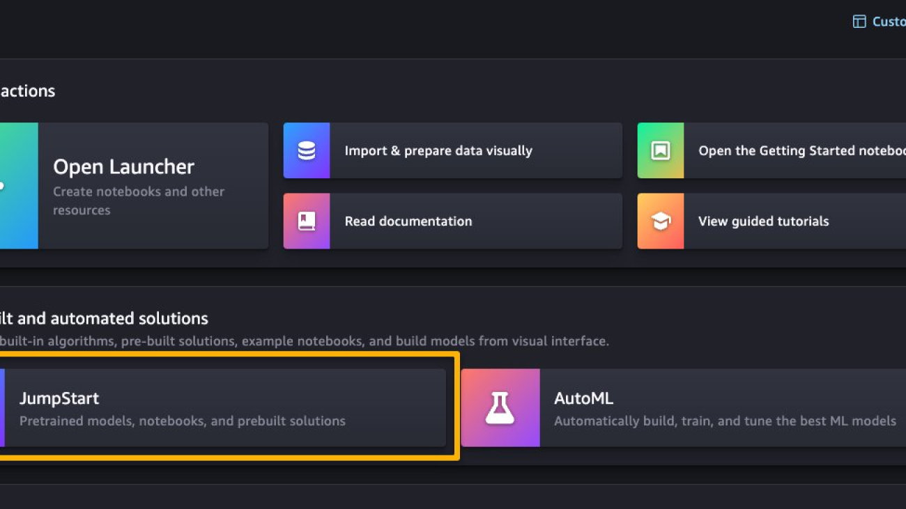
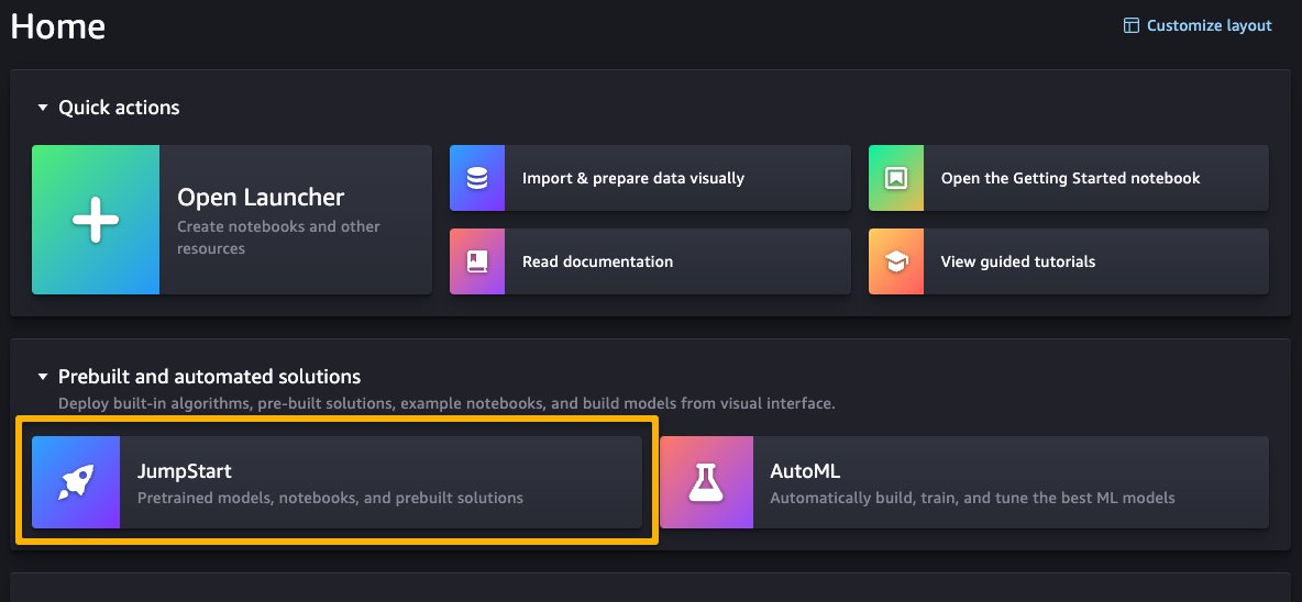
Once you’re on the SageMaker Studio UI, you can access SageMaker JumpStart, which contains pre-trained models, notebooks, and prebuilt solutions, under Prebuilt and automated solutions.

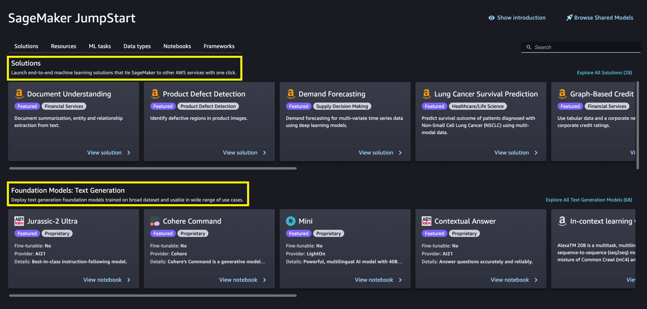
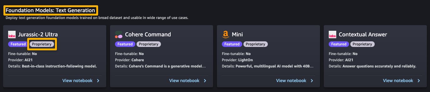
From the SageMaker JumpStart landing page, you can browse for solutions, models, notebooks, and other resources. The following screenshot shows an example of the landing page with solutions and foundation models listed.

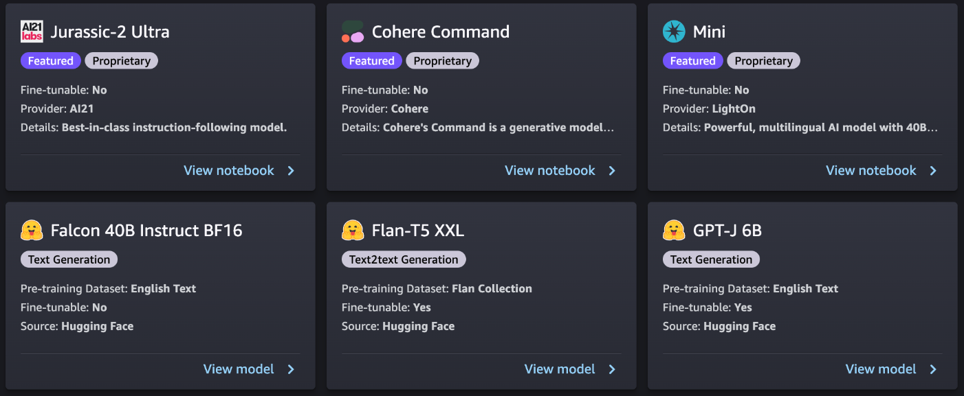
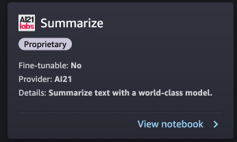
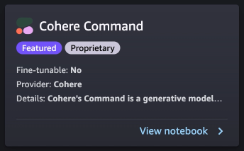
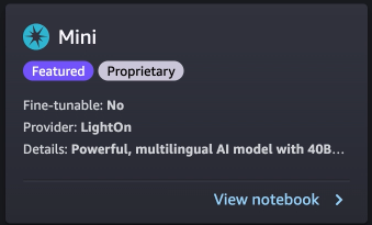
Each model has a model card, as shown in the following screenshot, which contains the model name, if it is fine-tunable or not, the provider name, and a short description about the model. You can also open the model card to learn more about the model and start training or deploying.

Subscribe in AWS Marketplace

Proprietary models in SageMaker JumpStart are published by model providers such as AI21, Cohere, and LightOn. You can identify proprietary models by the “Proprietary” tag on model cards, as shown in the following screenshot.

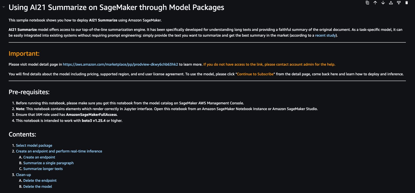
You can choose View notebook on the model card to open the notebook in read-only mode, as shown in the following screenshot. You can read the notebook for important information regarding prerequisites and other usage instructions.

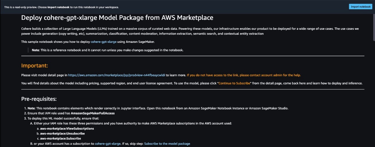
After importing the notebook, you need to select the appropriate notebook environment (image, kernel, instance type, and so on) before running codes. You should also follow the subscription and usage instructions per the selected notebook.

Before using a proprietary model, you need to first subscribe to the model from AWS Marketplace:

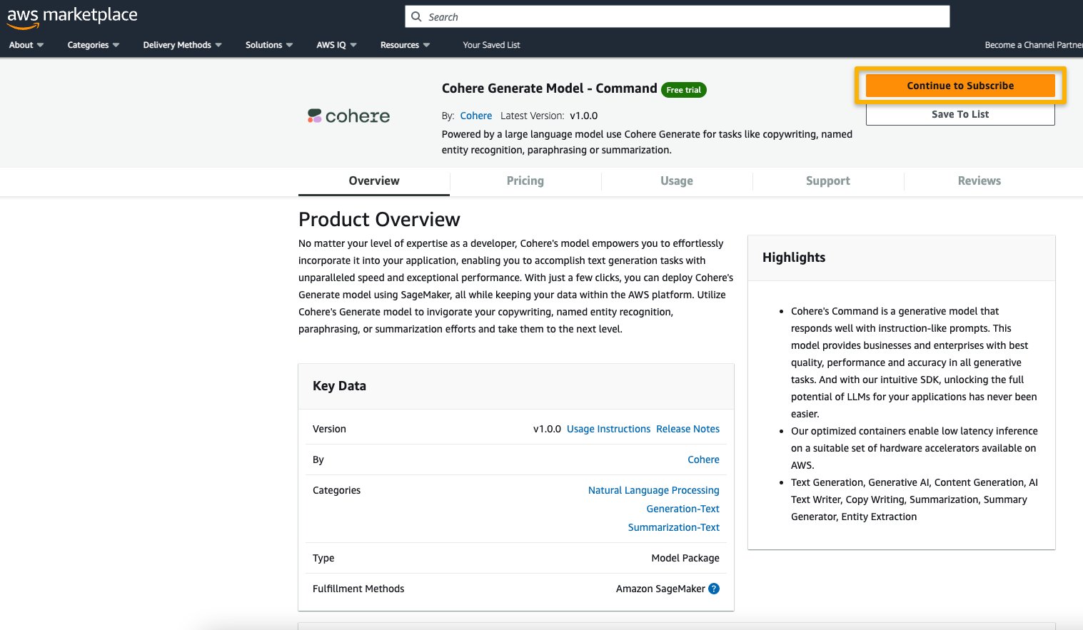
  1. Open the model listing page in AWS Marketplace.

The URL is provided in the Important section of the notebook, or you can access it from the SageMaker JumpStart service page. The listing page shows the overview, pricing, usage, and support information about the model.

  1. On the AWS Marketplace listing, choose Continue to subscribe.

If you don’t have the necessary permissions to view or subscribe to the model, reach out to your IT admin or procurement point of contact to subscribe to the model for you. Many enterprises may limit AWS Marketplace permissions to control the actions that someone with those permissions can take in the AWS Marketplace Management Portal.

  1. On the Subscribe to this software page, review the details and choose Accept offer if you and your organization agree with the EULA, pricing, and support terms.

If you have any questions or a request for volume discount, reach out to the model provider directly via the support email provided on the detail page or reach out to your AWS account team.

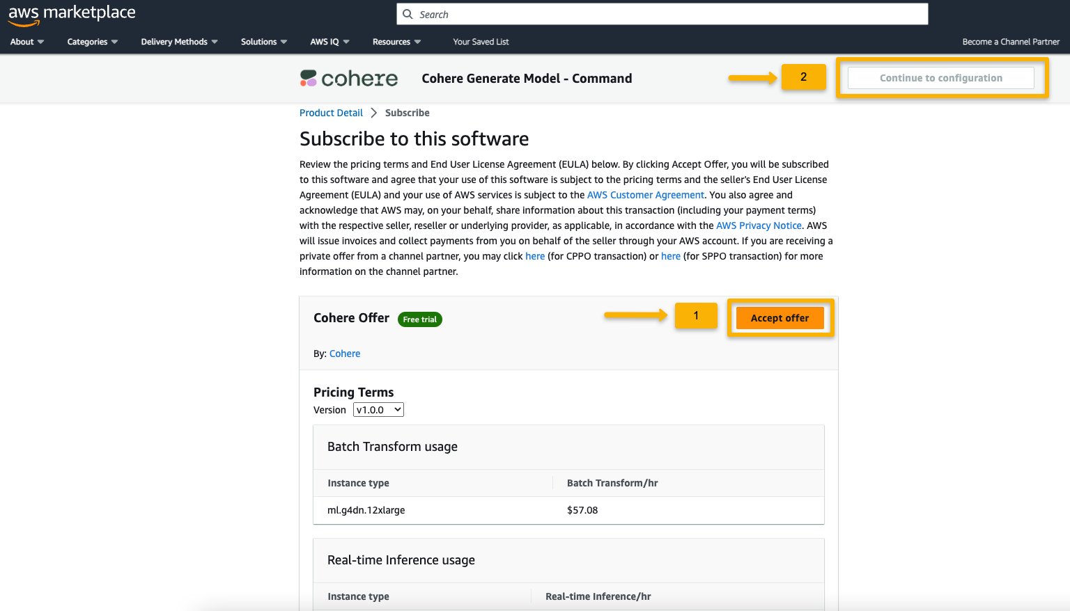
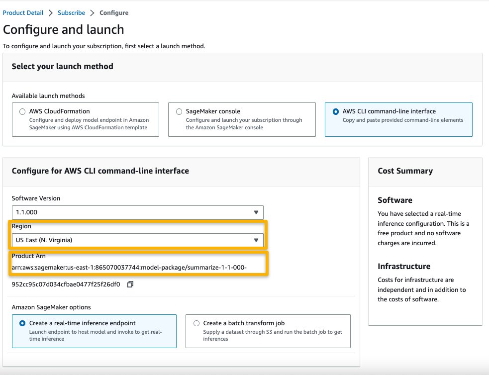
  1. Choose Continue to configuration and choose a Region.

You will see a product ARN displayed. This is the model package ARN that you need to specify while creating a deployable model using Boto3.

  1. Copy the ARN corresponding to your Region and specify the same in the notebook’s cell instruction.

Sample inferencing with sample prompts

Let’s look at some of the sample foundation models from A21 Labs, Cohere, and LightOn that are discoverable from SageMaker JumpStart in SageMaker Studio. All of them have same the instructions to subscribe from AWS Marketplace and import and configure the notebook.

AI21 Summarize

The Summarize model by A121 Labs condenses lengthy texts into short, easy-to-read bites that remain factually consistent with the source. The model is trained to generate summaries that capture key ideas based on a body of text. It doesn’t require any prompting. You simply input the text that needs to be summarized. Your source text can contain up to 50,000 characters, translating to roughly 10,000 words, or an impressive 40 pages.

The sample notebook for AI21 Summarize model provides important prerequisites that needs to be followed. For example the model is subscribed from AWS Marketplace , have appropriate IAM roles permissions, and required boto3 version etc. It walks you through how to select the model package, create endpoints for real-time inference, and then clean up.

The selected model package contains the mapping of ARNs to Regions. This is the information you captured after choosing Continue to configuration on the AWS Marketplace subscription page (in the section Evaluate and subscribe in Marketplace) and then selecting a Region for which you will see the corresponding product ARN.

The notebook may already have ARN prepopulated.

You then import some libraries required to run this notebook and install wikipedia, which is a Python library that makes it easy to access and parse data from Wikipedia. The notebook uses this later to showcase how to summarize a long text from Wikipedia.

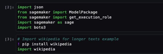
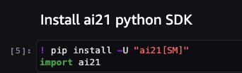
The notebook also proceeds to install the ai21 Python SDK, which is a wrapper around SageMaker APIs such as deploy and invoke endpoint.

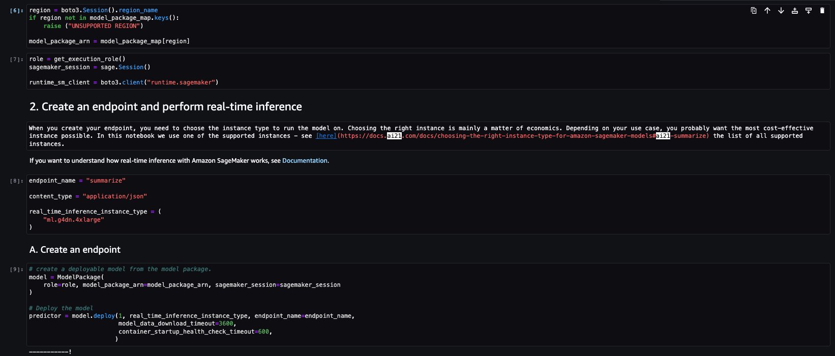
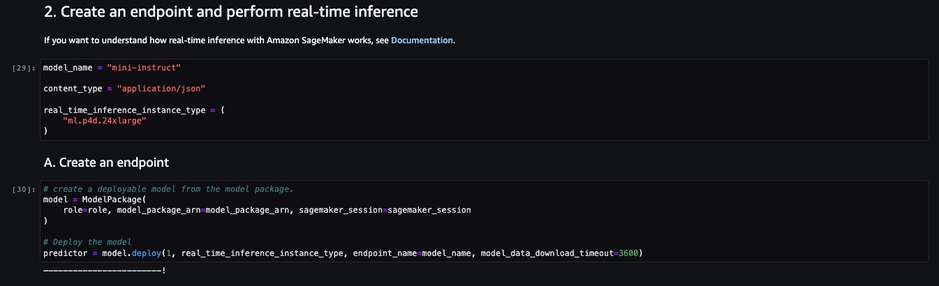
The next few cells of the notebook walk through the following steps:

  • Select the Region and fetch the model package ARN from model package map
  • Create your inference endpoint by selecting an instance type (depending on your use case and supported instance for the model; see Task-specific models for more details) to run the model on
  • Create a deployable model from the model package

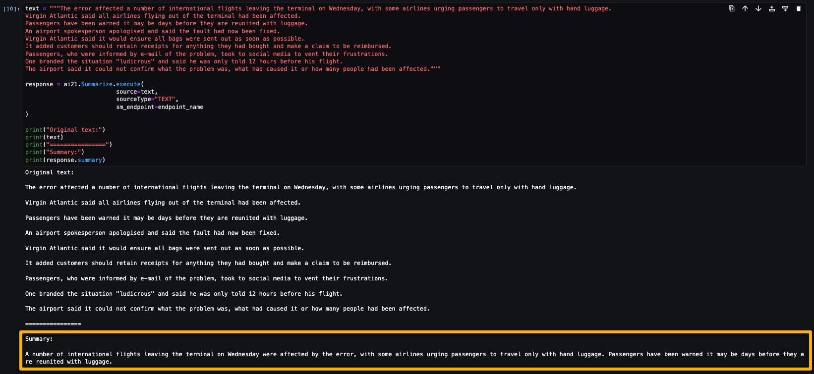
Let’s run the inference to generate a summary of a single paragraph taken from a news article. As you can see in the output, the summarized text is presented as an output by the model.

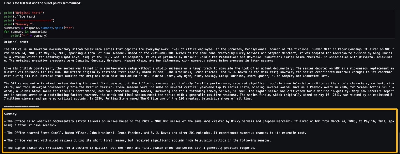
AI21 Summarize can handle inputs up to 50,000 characters. This translates into roughly 10,000 words, or 40 pages. As a demonstration of the model’s behavior, we load a page from Wikipedia.

Now that you have performed a real-time inference for testing, you may not need the endpoint anymore. You can delete the endpoint to avoid being charged.

Cohere Command

Cohere Command is a generative model that responds well with instruction-like prompts. This model provides businesses and enterprises with best quality, performance, and accuracy in all generative tasks. You can use Cohere’s Command model to invigorate your copywriting, named entity recognition, paraphrasing, or summarization efforts and take them to the next level.

The sample notebook for Cohere Command model provides important prerequisites that needs to be followed. For example the model is subscribed from AWS Marketplace, have appropriate IAM roles permissions, and required boto3 version etc. It walks you through how to select the model package, create endpoints for real-time inference, and then clean up.

Some of the tasks are similar to those covered in the previous notebook example, like installing Boto3, installing cohere-sagemaker (the package provides functionality developed to simplify interfacing with the Cohere model), and getting the session and Region.

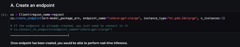
Let’s explore creating the endpoint. You provide the model package ARN, endpoint name, instance type to be used, and number of instances. Once created, the endpoint appears in your endpoint section of SageMaker.

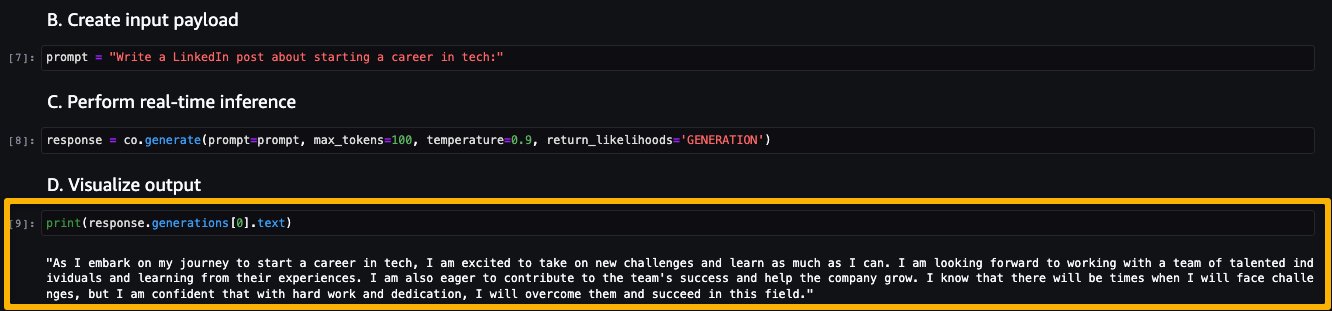
Now let’s run the inference to see some of the outputs from the Command model.

The following screenshot shows a sample example of generating a job post and its output. As you can see, the model generated a post from the given prompt.

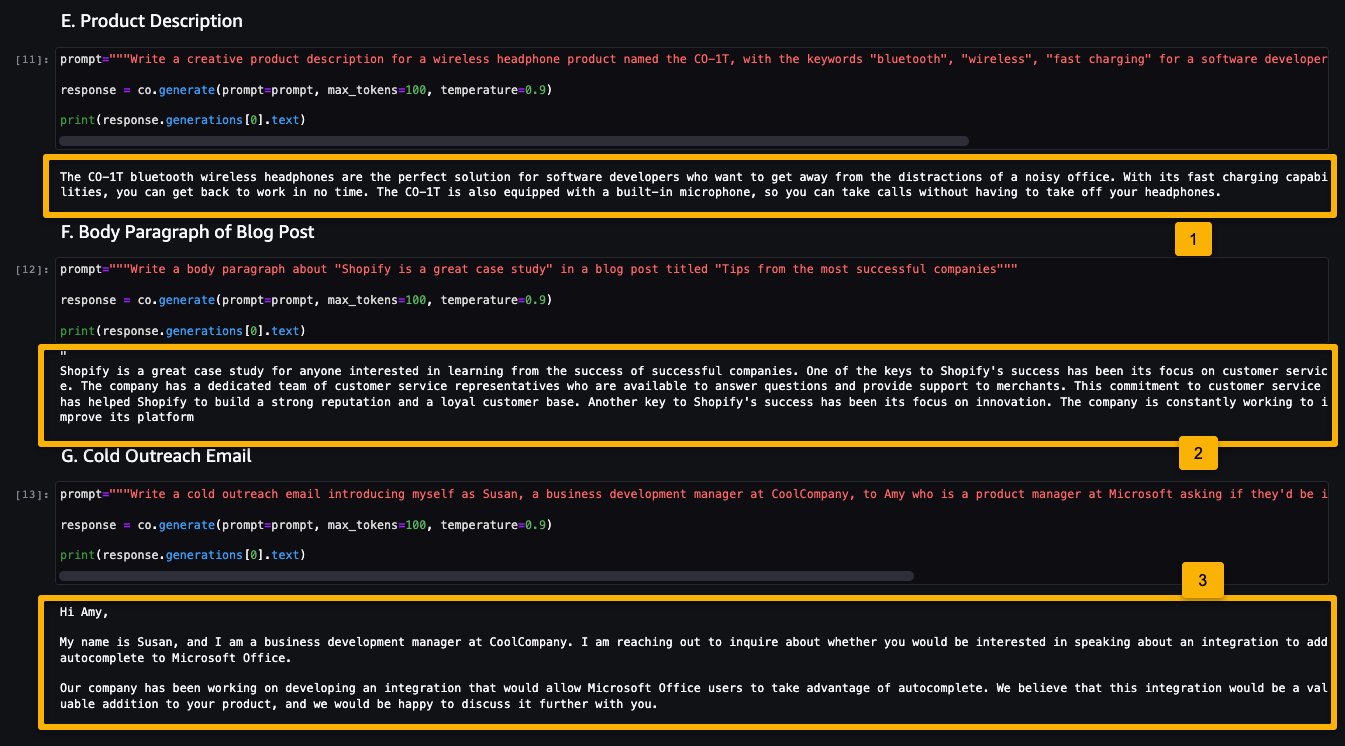
Now let’s look at the following examples:

  • Generate a product description
  • Generate a body paragraph of a blog post
  • Generate an outreach email

As you can see, the Cohere Command model generated text for various generative tasks.

Now that you have performed real-time inference for testing, you may not need the endpoint anymore. You can delete the endpoint to avoid being charged.

LightOn Mini-instruct

Mini-instruct, an AI model with 40 billion billion parameters created by LightOn, is a powerful multilingual AI system that has been trained using high-quality data from numerous sources. It is built to understand natural language and react to commands that are specific to your needs. It performs admirably in consumer products like voice assistants, chatbots, and smart appliances. It also has a wide range of business applications, including agent assistance and natural language production for automated customer care.

The sample notebook for LightOn Mini-instruct model provides important prerequisites that needs to be followed. For example the model is subscribed from AWS Marketplace, have appropriate IAM roles permissions, and required boto3 version etc. It walks you through how to select the model package, create endpoints for real-time inference, and then clean up.

Some of the tasks are similar to those covered in the previous notebook example, like installing Boto3 and getting the session Region.

Let’s look at creating the endpoint. First, provide the model package ARN, endpoint name, instance type to be used, and number of instances. Once created, the endpoint appears in your endpoint section of SageMaker.

Now let’s try inferencing the model by asking it to generate a list of ideas for articles for a topic, in this case watercolor.

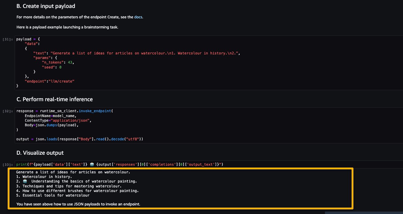
As you can see, the LightOn Mini-instruct model was able to provide generated text based on the given prompt.
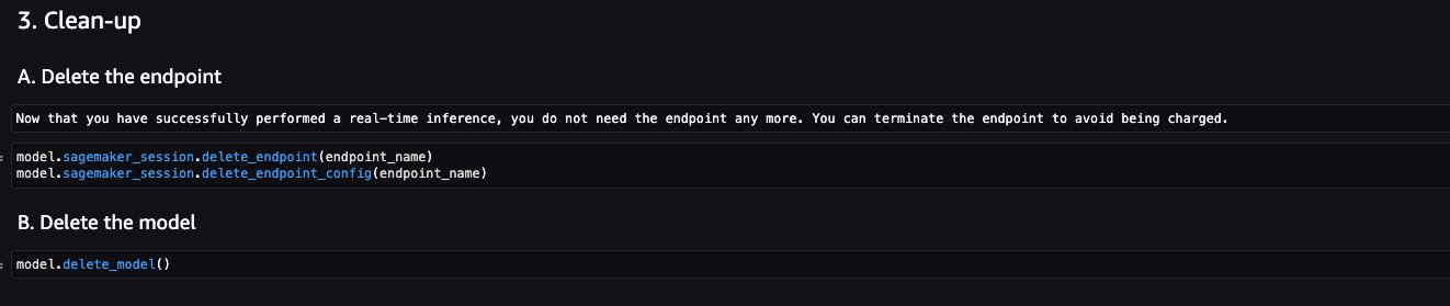
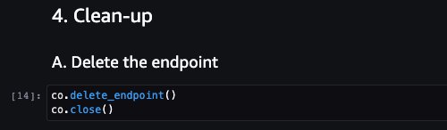
Clean up

After you have tested the models and created endpoints above for the example proprietary Foundation Models, make sure you delete the SageMaker inference endpoints and delete the models to avoid incurring charges.

Conclusion

In this post, we showed you how to get started with proprietary models from model providers such as AI21, Cohere, and LightOn in SageMaker Studio. Customers can discover and use proprietary Foundation Models in SageMaker JumpStart from Studio, the SageMaker SDK, and the SageMaker Console. With this, they have access to large-scale ML models that contain billions of parameters and are pretrained on terabytes of text and image data so customers can perform a wide range of tasks such as article summarization and text, image, or video generation. Because foundation models are pretrained, they can also help lower training and infrastructure costs and enable customization for your use case.

Resources


About the authors

June Won is a product manager with SageMaker JumpStart. He focuses on making foundation models easily discoverable and usable to help customers build generative AI applications.

Mani Khanuja is an Artificial Intelligence and Machine Learning Specialist SA at Amazon Web Services (AWS). She helps customers using machine learning to solve their business challenges using the AWS. She spends most of her time diving deep and teaching customers on AI/ML projects related to computer vision, natural language processing, forecasting, ML at the edge, and more. She is passionate about ML at edge, therefore, she has created her own lab with self-driving kit and prototype manufacturing production line, where she spends lot of her free time.

Nitin Eusebius is a Sr. Enterprise Solutions Architect at AWS with experience in Software Engineering , Enterprise Architecture and AI/ML. He works with customers on helping them build well-architected applications on the AWS platform. He is passionate about solving technology challenges and helping customers with their cloud journey.

Read More

How Earth.com and Provectus implemented their MLOps Infrastructure with Amazon SageMaker

How Earth.com and Provectus implemented their MLOps Infrastructure with Amazon SageMaker

This blog post is co-written with Marat Adayev and Dmitrii Evstiukhin from Provectus.

When machine learning (ML) models are deployed into production and employed to drive business decisions, the challenge often lies in the operation and management of multiple models. Machine Learning Operations (MLOps) provides the technical solution to this issue, assisting organizations in managing, monitoring, deploying, and governing their models on a centralized platform.

At-scale, real-time image recognition is a complex technical problem that also requires the implementation of MLOps. By enabling effective management of the ML lifecycle, MLOps can help account for various alterations in data, models, and concepts that the development of real-time image recognition applications is associated with.

One such application is EarthSnap, an AI-powered image recognition application that enables users to identify all types of plants and animals, using the camera on their smartphone. EarthSnap was developed by Earth.com, a leading online platform for enthusiasts who are passionate about the environment, nature, and science.

Earth.com’s leadership team recognized the vast potential of EarthSnap and set out to create an application that utilizes the latest deep learning (DL) architectures for computer vision (CV). However, they faced challenges in managing and scaling their ML system, which consisted of various siloed ML and infrastructure components that had to be maintained manually. They needed a cloud platform and a strategic partner with proven expertise in delivering production-ready AI/ML solutions, to quickly bring EarthSnap to the market. That is where Provectus, an AWS Premier Consulting Partner with competencies in Machine Learning, Data & Analytics, and DevOps, stepped in.

This post explains how Provectus and Earth.com were able to enhance the AI-powered image recognition capabilities of EarthSnap, reduce engineering heavy lifting, and minimize administrative costs by implementing end-to-end ML pipelines, delivered as part of a managed MLOps platform and managed AI services.

Challenges faced in the initial approach

The executive team at Earth.com was eager to accelerate the launch of EarthSnap. They swiftly began to work on AI/ML capabilities by building image recognition models using Amazon SageMaker. The following diagram shows the initial image recognition ML workflow, run manually and sequentially.

The models developed by Earth.com lived across various notebooks. They required the manual sequential execution run of a series of complex notebooks to process the data and retrain the model. Endpoints had to be deployed manually as well.

Earth.com didn’t have an in-house ML engineering team, which made it hard to add new datasets featuring new species, release and improve new models, and scale their disjointed ML system.

The ML components for data ingestion, preprocessing, and model training were available as disjointed Python scripts and notebooks, which required a lot of manual heavy lifting on the part of engineers.

The initial solution also required the support of a technical third party, to release new models swiftly and efficiently.

First iteration of the solution

Provectus served as a valuable collaborator for Earth.com, playing a crucial role in augmenting the AI-driven image recognition features of EarthSnap. The application’s workflows were automated by implementing end-to-end ML pipelines, which were delivered as part of Provectus’s managed MLOps platform and supported through managed AI services.

A series of project discovery sessions were initiated by Provectus to examine EarthSnap’s existing codebase and inventory the notebook scripts, with the goal of reproducing the existing model results. After the model results had been restored, the scattered components of the ML workflow were merged into an automated ML pipeline using Amazon SageMaker Pipelines, a purpose-built CI/CD service for ML.

The final pipeline includes the following components:

  • Data QA & versioning – This step run as a SageMaker Processing job, ingests the source data from Amazon Simple Storage Service (Amazon S3) and prepares the metadata for the next step, containing only valid images (URI and label) that are filtered according to internal rules. It also persists a manifest file to Amazon S3, including all necessary information to recreate that dataset version.
  • Data preprocessing – This includes multiple steps wrapped as SageMaker processing jobs, and run sequentially. The steps preprocess the images, convert them to RecordIO format, split the images into datasets (full, train, test and validation), and prepare the images to be consumed by SageMaker training jobs.
  • Hyperparameter tuning – A SageMaker hyperparameter tuning job takes as input a subset of the training and validation set and runs a series of small training jobs under the hood to determine the best parameters for the full training job.
  • Full training – A step SageMaker training job launches the training job on the entire data, given the best parameters from the hyperparameter tuning step.
  • Model evaluation – A step SageMaker processing job is run after the final model has been trained. This step produces an expanded report containing the model’s metrics.
  • Model creation – The SageMaker ModelCreate step wraps the model into the SageMaker model package and pushes it to the SageMaker model registry.

All steps are run in an automated manner after the pipeline has been run. The pipeline can be run via any of following methods:

  • Automatically using AWS CodeBuild, after the new changes are pushed to a primary branch and a new version of the pipeline is upserted (CI)
  • Automatically using Amazon API Gateway, which can be triggered with a certain API call
  • Manually in Amazon SageMaker Studio

After the pipeline run (launched using one of preceding methods), a trained model is produced that is ready to be deployed as a SageMaker endpoint. This means that the model must first be approved by the PM or engineer in the model registry, then the model is automatically rolled out to the stage environment using Amazon EventBridge and tested internally. After the model is confirmed to be working as expected, it’s deployed to the production environment (CD).

The Provectus solution for EarthSnap can be summarized in the following steps:

  • Start with fully automated, end-to-end ML pipelines to make it easier for Earth.com to release new models
  • Build on top of the pipelines to deliver a robust ML infrastructure for the MLOps platform, featuring all components for streamlining AI/ML
  • Support the solution by providing managed AI services (including ML infrastructure provisioning, maintenance, and cost monitoring and optimization)
  • Bring EarthSnap to its desired state (mobile application and backend) through a series of engagements, including AI/ML work, data and database operations, and DevOps

After the foundational infrastructure and processes were established, the model was trained and retrained on a larger dataset. At this point, however, the team encountered an additional issue when attempting to expand the model with even larger datasets. We needed to find a way to restructure the solution architecture, making it more sophisticated and capable of scaling effectively. The following diagram shows the EarthSnap AI/ML architecture.

The AI/ML architecture for EarthSnap is designed around a series of AWS services:

  • Sagemaker Pipeline runs using one of the methods mentioned above (CodeBuild, API, manual) that trains the model and produces artifacts and metrics. As a result, the new version of the model is pushed to the Sagemaker Model registry
  • Then the model is reviewed by an internal team (PM/engineer) in model registry and approved/rejected based on metrics provided
  • Once the model is approved, the model version is automatically deployed to the stage environment using the Amazon EventBridge that tracks the model status change
  • The model is deployed to the production environment if the model passes all tests in the stage environment

Final solution

To accommodate all necessary sets of labels, the solution for EarthSnap’s model required substantial modifications, because incorporating all species within a single model proved to be both costly and inefficient. The plant category was selected first for implementation.

A thorough examination of plant data was conducted, to organize it into subsets based on shared internal characteristics. The solution for the plant model was redesigned by implementing a multi-model parent/child architecture. This was achieved by training child models on grouped subsets of plant data and training the parent model on a set of data samples from each subcategory. The Child models were employed for accurate classification within the internally grouped species, while the parent model was utilized to categorize input plant images into subgroups. This design necessitated distinct training processes for each model, leading to the creation of separate ML pipelines. With this new design, along with the previously established ML/MLOps foundation, the EarthSnap application was able to encompass all essential plant species, resulting in improved efficiency concerning model maintenance and retraining. The following diagram illustrates the logical scheme of parent/child model relations.

Upon completing the redesign, the ultimate challenge was to guarantee that the AI solution powering EarthSnap could manage the substantial load generated by a broad user base. Fortunately, the managed AI onboarding process encompasses all essential automation, monitoring, and procedures for transitioning the solution into a production-ready state, eliminating the need for any further capital investment.

Results

Despite the pressing requirement to develop and implement the AI-driven image recognition features of EarthSnap within a few months, Provectus managed to meet all project requirements within the designated time frame. In just 3 months, Provectus modernized and productionized the ML solution for EarthSnap, ensuring that their mobile application was ready for public release.

The modernized infrastructure for ML and MLOps allowed Earth.com to reduce engineering heavy lifting and minimize the administrative costs associated with maintenance and support of EarthSnap. By streamlining processes and implementing best practices for CI/CD and DevOps, Provectus ensured that EarthSnap could achieve better performance while improving its adaptability, resilience, and security. With a focus on innovation and efficiency, we enabled EarthSnap to function flawlessly, while providing a seamless and user-friendly experience for all users.

As part of its managed AI services, Provectus was able to reduce the infrastructure management overhead, establish well-defined SLAs and processes, ensure 24/7 coverage and support, and increase overall infrastructure stability, including production workloads and critical releases. We initiated a series of enhancements to deliver managed MLOps platform and augment ML engineering. Specifically, it now takes Earth.com minutes, instead of several days, to release new ML models for their AI-powered image recognition application.

With assistance from Provectus, Earth.com was able to release its EarthSnap application at the Apple Store and Playstore ahead of schedule. The early release signified the importance of Provectus’ comprehensive work for the client.

”I’m incredibly excited to work with Provectus. Words can’t describe how great I feel about handing over control of the technical side of business to Provectus. It is a huge relief knowing that I don’t have to worry about anything other than developing the business side.”

– Eric Ralls, Founder and CEO of EarthSnap.

The next steps of our cooperation will include: adding advanced monitoring components to pipelines, enhancing model retraining, and introducing a human-in-the-loop step.

Conclusion

The Provectus team hopes that Earth.com will continue to modernize EarthSnap with us. We look forward to powering the company’s future expansion, further popularizing natural phenomena, and doing our part to protect our planet.

To learn more about the Provectus ML infrastructure and MLOps, visit Machine Learning Infrastructure and watch the webinar for more practical advice. You can also learn more about Provectus managed AI services at the Managed AI Services.

If you’re interested in building a robust infrastructure for ML and MLOps in your organization, apply for the ML Acceleration Program to get started.

Provectus helps companies in healthcare and life sciences, retail and CPG, media and entertainment, and manufacturing, achieve their objectives through AI.

Provectus is an AWS Machine Learning Competency Partner and AI-first transformation consultancy and solutions provider helping design, architect, migrate, or build cloud-native applications on AWS.

Contact Provectus | Partner Overview


About the Authors

Marat Adayev is an ML Solutions Architect at Provectus
Dmitrii Evstiukhin is the Director of Managed Services at Provectus
James Burdon is a Senior Startups Solutions Architect at AWS

Read More

NVIDIA H100 GPUs Set Standard for Generative AI in Debut MLPerf Benchmark 

NVIDIA H100 GPUs Set Standard for Generative AI in Debut MLPerf Benchmark 

Leading users and industry-standard benchmarks agree: NVIDIA H100 Tensor Core GPUs deliver the best AI performance, especially on the large language models (LLMs) powering generative AI.

H100 GPUs set new records on all eight tests in the latest MLPerf training benchmarks released today, excelling on a new MLPerf test for generative AI. That excellence is delivered both per-accelerator and at-scale in massive servers.

For example, on a commercially available cluster of 3,584 H100 GPUs co-developed by startup Inflection AI and operated by CoreWeave, a cloud service provider specializing in GPU-accelerated workloads, the system completed the massive GPT-3-based training benchmark in less than eleven minutes.

“Our customers are building state-of-the-art generative AI and LLMs at scale today, thanks to our thousands of H100 GPUs on fast, low-latency InfiniBand networks,” said Brian Venturo, co-founder and CTO of CoreWeave. “Our joint MLPerf submission with NVIDIA clearly demonstrates the great performance our customers enjoy.”

Top Performance Available Today

Inflection AI harnessed that performance to build the advanced LLM behind its first personal AI, Pi, which stands for personal intelligence. The company will act as an AI studio, creating personal AIs users can interact with in simple, natural ways.

“Anyone can experience the power of a personal AI today based on our state-of-the-art large language model that was trained on CoreWeave’s powerful network of H100 GPUs,” said Mustafa Suleyman, CEO of Inflection AI.

Co-founded in early 2022 by Mustafa and Karén Simonyan of DeepMind and Reid Hoffman, Inflection AI aims to work with CoreWeave to build one of the largest computing clusters in the world using NVIDIA GPUs.

Tale of the Tape

These user experiences reflect the performance demonstrated in the MLPerf benchmarks announced today.

NVIDIA wins all eight tests in MLPerf Training v3.0

H100 GPUs delivered the highest performance on every benchmark, including large language models, recommenders, computer vision, medical imaging and speech recognition. They were the only chips to run all eight tests, demonstrating the versatility of the NVIDIA AI platform.

Excellence Running at Scale

Training is typically a job run at scale by many GPUs working in tandem. On every MLPerf test, H100 GPUs set new at-scale performance records for AI training.

Optimizations across the full technology stack enabled near linear performance scaling on the demanding LLM test as submissions scaled from hundreds to thousands of H100 GPUs.

NVIDIA demonstrates efficiency at scale in MLPerf Training v3.0

In addition, CoreWeave delivered from the cloud similar performance to what NVIDIA achieved from an AI supercomputer running in a local data center. That’s a testament to the low-latency networking of the NVIDIA Quantum-2 InfiniBand networking CoreWeave uses.

In this round, MLPerf also updated its benchmark for recommendation systems.

The new test uses a larger data set and a more modern AI model to better reflect the challenges cloud service providers face. NVIDIA was the only company to submit results on the enhanced benchmark.

An Expanding NVIDIA AI Ecosystem

Nearly a dozen companies submitted results on the NVIDIA platform in this round. Their work shows NVIDIA AI is backed by the industry’s broadest ecosystem in machine learning.

Submissions came from major system makers that include ASUS, Dell Technologies, GIGABYTE, Lenovo, and QCT. More than 30 submissions ran on H100 GPUs.

This level of participation lets users know they can get great performance with NVIDIA AI both in the cloud and in servers running in their own data centers.

Performance Across All Workloads

NVIDIA ecosystem partners participate in MLPerf because they know it’s a valuable tool for customers evaluating AI platforms and vendors.

The benchmarks cover workloads users care about — computer vision, translation and reinforcement learning, in addition to generative AI and recommendation systems.

Users can rely on MLPerf results to make informed buying decisions, because the tests are transparent and objective. The benchmarks enjoy backing from a broad group that includes Arm, Baidu, Facebook AI, Google, Harvard, Intel, Microsoft, Stanford and the University of Toronto.

MLPerf results are available today on H100, L4 and NVIDIA Jetson platforms across AI training, inference and HPC benchmarks. We’ll be making submissions on NVIDIA Grace Hopper systems in future MLPerf rounds as well.

The Importance of Energy Efficiency

As AI’s performance requirements grow, it’s essential to expand the efficiency of how that performance is achieved. That’s what accelerated computing does.

Data centers accelerated with NVIDIA GPUs use fewer server nodes, so they use less rack space and energy. In addition, accelerated networking boosts efficiency and performance, and ongoing software optimizations bring x-factor gains on the same hardware.

Energy-efficient performance is good for the planet and business, too. Increased performance can speed time to market and let organizations build more advanced applications.

Energy efficiency also reduces costs because data centers accelerated with NVIDIA GPUs use fewer server nodes. Indeed, NVIDIA powers 22 of the top 30 supercomputers on the latest Green500 list.

Software Available to All

NVIDIA AI Enterprise, the software layer of the NVIDIA AI platform, enables optimized performance on leading accelerated computing infrastructure. The software comes with the enterprise-grade support, security and reliability required to run AI in the corporate data center.

All the software used for these tests is available from the MLPerf repository, so virtually anyone can get these world-class results.

Optimizations are continuously folded into containers available on NGC, NVIDIA’s catalog for GPU-accelerated software.

Read this technical blog for a deeper dive into the optimizations fueling NVIDIA’s MLPerf performance and efficiency.

Read More