New tool helps watermark and identify synthetic images created by ImagenRead More
New tool helps watermark and identify synthetic images created by ImagenRead More
New tool helps watermark and identify synthetic images created by ImagenRead More

Today, in partnership with Google Cloud, we’re beta launching SynthID, a new tool for watermarking and identifying AI-generated images. It’s being released to a limited number of Vertex AI customers using Imagen, one of our latest text-to-image models that uses input text to create photorealistic images. This technology embeds a digital watermark directly into the pixels of an image, making it imperceptible to the human eye, but detectable for identification. While generative AI can unlock huge creative potential, it also presents new risks, like creators spreading false information — both intentionally or unintentionally. Being able to identify AI-generated content is critical to empowering people with knowledge of when they’re interacting with generated media, and for helping prevent the spread of misinformation.Read More
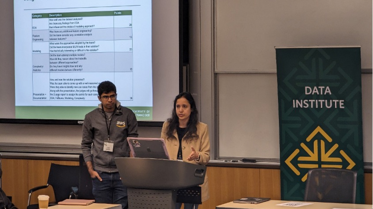
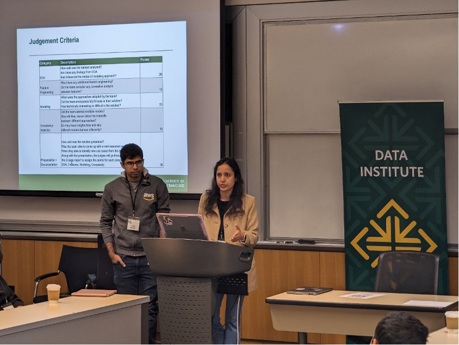
As part of the 2023 Data Science Conference (DSCO 23), AWS partnered with the Data Institute at the University of San Francisco (USF) to conduct a datathon. Participants, both high school and undergraduate students, competed on a data science project that focused on air quality and sustainability. The Data Institute at the USF aims to support cross-disciplinary research and education in the field of data science. The Data Institute and the Data Science Conference provide a distinctive fusion of cutting-edge academic research and the entrepreneurial culture of the technology industry in the San Francisco Bay Area.
The students used Amazon SageMaker Studio Lab, which is a free platform that provides a JupyterLab environment with compute (CPU and GPU) and storage (up to 15GB). Because most of the students were unfamiliar with machine learning (ML), they were given a brief tutorial illustrating how to set up an ML pipeline: how to conduct exploratory data analysis, feature engineering, model building, and model evaluation, and how to set up inference and monitoring. The tutorial referenced Amazon Sustainability Data Initiative (ASDI) datasets from the National Oceanic and Atmospheric Administration (NOAA) and OpenAQ to build an ML model to predict air quality levels using weather data via a binary classification AutoGluon model. Next, the students were turned loose to work on their own projects in their teams. The winning teams were led by Peter Ma, Ben Welner, and Ei Coltin, who were all awarded prizes at the opening ceremony of the Data Science Conference at USF.
“This was a fun event, and a great way to work with others. I learned some Python coding in class but this helped make it real. During the datathon, my team member and I conducted research on different ML models (LightGBM, logistic regression, SVM models, Random Forest Classifier, etc.) and their performance on an AQI dataset from NOAA aimed at detecting the toxicity of the atmosphere under specific weather conditions. We built a gradient boosting classifier to predict air quality from weather statistics.”
– Anay Pant, a junior at the Athenian School, Danville, California, and one of the winners of the datathon.
“AI is becoming increasingly important in the workplace, and 82% of companies need employees with machine learning skills. It’s critical that we develop the talent needed to build products and experiences that we will all benefit from, this includes software engineering, data science, domain knowledge, and more. We were thrilled to help the next generation of builders explore machine learning and experiment with its capabilities. Our hope is that they take this forward and expand their ML knowledge. I personally hope to one day use an app built by one of the students at this datathon!”
– Sherry Marcus, Director of AWS ML Solutions Lab.
“This is the first year we used SageMaker Studio Lab. We were pleased by how quickly high school/undergraduate students and our graduate student mentors could start their projects and collaborate using SageMaker Studio.”
– Diane Woodbridge from the Data Institute of the University of San Francisco.
If you missed this datathon, you can still register for your own Studio Lab account and work on your own project. If you’re interested in running your own hackathon, reach out to your AWS representative for a Studio Lab referral code, which will give your participants immediate access to the service. Finally, you can look for next year’s challenge at the USF Data Institute.

 Neha Narwal is a Machine Learning Engineer at AWS Bedrock where she contributes to development of large language models for generative AI applications. Her focus lies at the intersection of science and engineering to influence research in Natural Language Processing domain.
 Vidya Sagar Ravipati is a Applied Science Manager at the Generative AI Innovation Center, where he leverages his vast experience in large-scale distributed systems and his passion for machine learning to help AWS customers across different industry verticals accelerate their AI and cloud adoption.

The ability to detect objects in the visual world is crucial for computer vision and machine intelligence, enabling applications like adaptive autonomous agents and versatile shopping systems. However, modern object detectors are limited by the manual annotations of their training data, resulting in a vocabulary size significantly smaller than the vast array of objects encountered in reality. To overcome this, the open-vocabulary detection task (OVD) has emerged, utilizing image-text pairs for training and incorporating new category names at test time by associating them with the image content. By treating categories as text embeddings, open-vocabulary detectors can predict a wide range of unseen objects. Various techniques such as image-text pre-training, knowledge distillation, pseudo labeling, and frozen models, often employing convolutional neural network (CNN) backbones, have been proposed. With the growing popularity of vision transformers (ViTs), it is important to explore their potential for building proficient open-vocabulary detectors.
The existing approaches assume the availability of pre-trained vision-language models (VLMs) and focus on fine-tuning or distillation from these models to address the disparity between image-level pre-training and object-level fine-tuning. However, as VLMs are primarily designed for image-level tasks like classification and retrieval, they do not fully leverage the concept of objects or regions during the pre-training phase. Thus, it could be beneficial for open-vocabulary detection if we build locality information into the image-text pre-training.
In “RO-ViT: Region-Aware Pretraining for Open-Vocabulary Object Detection with Vision Transformers”, presented at CVPR 2023, we introduce a simple method to pre-train vision transformers in a region-aware manner to improve open-vocabulary detection. In vision transformers, positional embeddings are added to image patches to encode information about the spatial position of each patch within the image. Standard pre-training typically uses full-image positional embeddings, which does not generalize well to detection tasks. Thus, we propose a new positional embedding scheme, called “cropped positional embedding”, that better aligns with the use of region crops in detection fine-tuning. In addition, we replace the softmax cross entropy loss with focal loss in contrastive image-text learning, allowing us to learn from more challenging and informative examples. Finally, we leverage recent advances in novel object proposals to enhance open-vocabulary detection fine-tuning, which is motivated by the observation that existing methods often miss novel objects during the proposal stage due to overfitting to foreground categories. We are also releasing the code here.
Existing VLMs are trained to match an image as a whole to a text description. However, we observe there is a mismatch between the way the positional embeddings are used in the existing contrastive pre-training approaches and open-vocabulary detection. The positional embeddings are important to transformers as they provide the information of where each element in the set comes from. This information is often useful for downstream recognition and localization tasks. Pre-training approaches typically apply full-image positional embeddings during training, and use the same positional embeddings for downstream tasks, e.g., zero-shot recognition. However, the recognition occurs at region-level for open-vocabulary detection fine-tuning, which requires the full-image positional embeddings to generalize to regions that they never see during the pre-training.
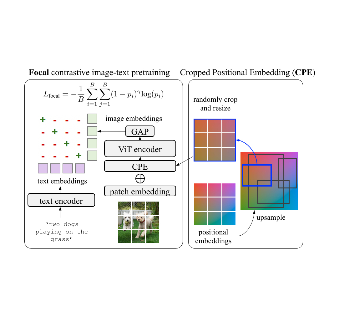
To address this, we propose cropped positional embeddings (CPE). With CPE, we upsample positional embeddings from the image size typical for pre-training, e.g., 224×224 pixels, to that typical for detection tasks, e.g., 1024×1024 pixels. Then we randomly crop and resize a region, and use it as the image-level positional embeddings during pre-training. The position, scale, and aspect ratio of the crop is randomly sampled. Intuitively, this causes the model to view an image not as a full image in itself, but as a region crop from some larger unknown image. This better matches the downstream use case of detection where recognition occurs at region- rather than image-level.
 |
| For the pre-training, we propose cropped positional embedding (CPE) which randomly crops and resizes a region of positional embeddings instead of using the whole-image positional embedding (PE). In addition, we use focal loss instead of the common softmax cross entropy loss for contrastive learning. |
We also find it beneficial to learn from hard examples with a focal loss. Focal loss enables finer control over how hard examples are weighted than what the softmax cross entropy loss can provide. We adopt the focal loss and replace it with the softmax cross entropy loss in both image-to-text and text-to-image losses. Both CPE and focal loss introduce no extra parameters and minimal computation costs.
An open-vocabulary detector is trained with the detection labels of ‘base’ categories, but needs to detect the union of ‘base’ and ‘novel’ (unlabeled) categories at test time. Despite the backbone features pre-trained from the vast open-vocabulary data, the added detector layers (neck and heads) are newly trained with the downstream detection dataset. Existing approaches often miss novel/unlabeled objects in the object proposal stage because the proposals tend to classify them as background. To remedy this, we leverage recent advances in a novel object proposal method and adopt the localization quality-based objectness (i.e., centerness score) instead of object-or-not binary classification score, which is combined with the detection score. During training, we compute the detection scores for each detected region as the cosine similarity between the region’s embedding (computed via RoI-Align operation) and the text embeddings of the base categories. At test time, we append the text embeddings of novel categories, and the detection score is now computed with the union of the base and novel categories.
 |
| The pre-trained ViT backbone is transferred to the downstream open-vocabulary detection by replacing the global average pooling with detector heads. The RoI-Align embeddings are matched with the cached category embeddings to obtain the VLM score, which is combined with the detection score into the open-vocabulary detection score. |
We evaluate RO-ViT on the LVIS open-vocabulary detection benchmark. At the system-level, our best model achieves 33.6 box average precision on rare categories (APr) and 32.1 mask APr, which outperforms the best existing ViT-based approach OWL-ViT by 8.0 APr and the best CNN-based approach ViLD-Ens by 5.8 mask APr. It also exceeds the performance of many other approaches based on knowledge distillation, pre-training, or joint training with weak supervision.
 |
| RO-ViT outperforms both the state-of-the-art (SOTA) ViT-based and CNN-based methods on LVIS open-vocabulary detection benchmark. We show mask AP on rare categories (APr) , except for SOTA ViT-based (OwL-ViT) where we show box AP. |
Apart from evaluating region-level representation through open-vocabulary detection, we evaluate the image-level representation of RO-ViT in image-text retrieval through the MS-COCO and Flickr30K benchmarks. Our model with 303M ViT outperforms the state-of-the-art CoCa model with 1B ViT on MS COCO, and is on par on Flickr30K. This shows that our pre-training method not only improves the region-level representation but also the global image-level representation for retrieval.
 |
| We show zero-shot image-text retrieval on MS COCO and Flickr30K benchmarks, and compare with dual-encoder methods. We report recall@1 (top-1 recall) on image-to-text (I2T) and text-to-image (T2I) retrieval tasks. RO-ViT outperforms the state-of-the-art CoCa with the same backbone. |
 |
| RO-ViT open-vocabulary detection on LVIS. We only show the novel categories for clarity. RO-ViT detects many novel categories that it has never seen during detection training: “fishbowl”, “sombrero”, “persimmon”, “gargoyle”. |
We visualize and compare the learned positional embeddings of RO-ViT with the baseline. Each tile is the cosine similarity between positional embeddings of one patch and all other patches. For example, the tile in the top-left corner (marked in red) visualizes the similarity between the positional embedding of the location (row=1, column=1) and those positional embeddings of all other locations in 2D. The brightness of the patch indicates how close the learned positional embeddings of different locations are. RO-ViT forms more distinct clusters at different patch locations showing symmetrical global patterns around the center patch.
 |
| Each tile shows the cosine similarity between the positional embedding of the patch (at the indicated row-column position) and the positional embeddings of all other patches. ViT-B/16 backbone is used. |
We present RO-ViT, a contrastive image-text pre-training framework to bridge the gap between image-level pre-training and open-vocabulary detection fine-tuning. Our methods are simple, scalable, and easy to apply to any contrastive backbones with minimal computation overhead and no increase in parameters. RO-ViT achieves the state-of-the-art on LVIS open-vocabulary detection benchmark and on the image-text retrieval benchmarks, showing the learned representation is not only beneficial at region-level but also highly effective at the image-level. We hope this study can help the research on open-vocabulary detection from the perspective of image-text pre-training which can benefit both region-level and image-level tasks.
Dahun Kim, Anelia Angelova, and Weicheng Kuo conducted this work and are now at Google DeepMind. We would like to thank our colleagues at Google Research for their advice and helpful discussions.
AWS service enables machine learning innovation on a robust foundation.Read More
Companies are discovering how accelerated computing can boost their bottom lines while making a positive impact on the planet.
The NVIDIA RAPIDS Accelerator for Apache Spark, software that speeds data analytics, not only raises performance and lowers costs, it increases energy efficiency, too. That means it can help companies meet goals for net-zero emissions of greenhouse gases like carbon dioxide.
A new benchmark shows that the RAPIDS Accelerator can reduce a company’s carbon footprint by as much as 80% while delivering 5x average speedups and 4x reductions in computing costs.
That’s a big win many can enjoy. Thousands of companies, including 80% of the Fortune 500, use Apache Spark to analyze their growing mountains of data.
In fact, if every Apache Spark user adopted the RAPIDS Accelerator, they could collectively reduce carbon dioxide emissions by a whopping 7.8 metric tons a year — or the amount of emissions a car produces on 878 gallons of gas. It’s a great example of how green computing can advance the fight against climate change.
More than 70 countries have set a net-zero target for greenhouse gas emissions, according to the United Nations. It describes the transition to net-zero as “one of the greatest challenges humankind has faced.”
Companies are getting on board, too.
For example, NVIDIA is working with a large financial services company to test Apache Spark for real-time fraud protection. The company hopes to lower its carbon footprint with accelerated computing so it can align with groups like the Net-Zero Banking Alliance.
One of the world’s largest AI supercomputers validated the energy efficiency of accelerated computing in May.
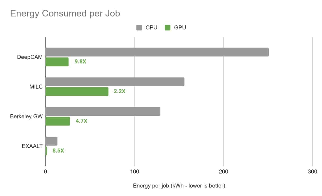
Across four popular scientific applications, the Perlmutter system at the National Energy Research Scientific Computing Center (NERSC) reported energy efficiency gains of 5x on average, thanks to NVIDIA A100 Tensor Core GPUs. An application for weather forecasting logged speed-ups of 9.8x compared to CPUs.
Organizations like AT&T, Adobe and the Internal Revenue Service have already discovered the performance and cost benefits of the RAPIDS Accelerator.
In a test last year, AT&T processed a month’s worth of mobile data — 2.8 trillion rows of information — in just five hours. That’s 3.3x faster at 60% lower cost than any prior test.
“It was a ‘wow’ moment because on CPU clusters, it takes more than 48 hours to process just seven days of data — in the past, we had the data but couldn’t use it because it took such a long time to process it,” said Abhay Dabholkar, an AI architect at AT&T, in a blog.
“We recommend that if a job is taking too long and you have a lot of data, turn on GPUs — with Spark, the same code that runs on CPUs runs on GPUs,” he added.
Adobe used accelerated computing on its Intelligent Services platform, which helps marketing teams speed analytics with AI.
It found that, using the RAPIDS Accelerator, a single NVIDIA GPU node could outperform a 16-node CPU cluster by 33% while slashing computing costs by 70%.
In a separate test, GPU-accelerated RAPIDS libraries trained an AI model 7x faster, saving 90% of the cost of running the same job on CPUs.
“This is an amazing cost savings and speed-up,” said Lei Zhang, a machine learning engineer at Adobe in a talk at GTC (free with registration).
CPUs weren’t powerful enough to ingest the 3+ terabyte dataset it needed to analyze, so the IRS turned to the RAPIDS Accelerator.
A Spark cluster of GPU-powered servers processed the load and opened the door to tackling even bigger datasets.
“We’re currently implementing this integration and already seeing over 20x speed improvements at half the cost for our data engineering and data science workflows,” said Joe Ansaldi, technical branch chief of the research and applied analytics and statistics division at the IRS, in a blog.
Performance speedups and cost savings vary across workloads. That’s why NVIDIA offers an accelerated Spark analysis tool.
The tool shows users what the RAPIDS Accelerator can deliver on their applications without any code changes. It also helps users tune GPU acceleration to get the best results on their workloads.
Once the RAPIDS Accelerator is boosting the bottom line, companies can calculate their energy savings and report their progress in protecting the planet.
Learn more in this solution brief. And watch the video below to see how the Cloudera Data Platform delivered a 44x speedup with the RAPIDS Accelerator for Apache Spark.
Get enterprise-grade security & privacy and the most powerful version of ChatGPT yet.OpenAI Blog
AB testing aids business operators with their decision making, and is considered the gold standard method for learning from data to improve digital user experiences. However, there is usually a gap between the requirements of practitioners, and the constraints imposed by the statistical hypothesis testing methodologies commonly used for analysis of AB tests. These include the lack of statistical power in multivariate designs with many factors, correlations between these factors, the need of sequential testing for early stopping, and the inability to pool knowledge from past tests. Here, we…Apple Machine Learning Research

Google’s Responsible AI research is built on a foundation of collaboration — between teams with diverse backgrounds and expertise, between researchers and product developers, and ultimately with the community at large. The Perception Fairness team drives progress by combining deep subject-matter expertise in both computer vision and machine learning (ML) fairness with direct connections to the researchers building the perception systems that power products across Google and beyond. Together, we are working to intentionally design our systems to be inclusive from the ground up, guided by Google’s AI Principles.
 |
| Perception Fairness research spans the design, development, and deployment of advanced multimodal models including the latest foundation and generative models powering Google’s products. |
Our team’s mission is to advance the frontiers of fairness and inclusion in multimodal ML systems, especially related to foundation models and generative AI. This encompasses core technology components including classification, localization, captioning, retrieval, visual question answering, text-to-image or text-to-video generation, and generative image and video editing. We believe that fairness and inclusion can and should be top-line performance goals for these applications. Our research is focused on unlocking novel analyses and mitigations that enable us to proactively design for these objectives throughout the development cycle. We answer core questions, such as: How can we use ML to responsibly and faithfully model human perception of demographic, cultural, and social identities in order to promote fairness and inclusion? What kinds of system biases (e.g., underperforming on images of people with certain skin tones) can we measure and how can we use these metrics to design better algorithms? How can we build more inclusive algorithms and systems and react quickly when failures occur?
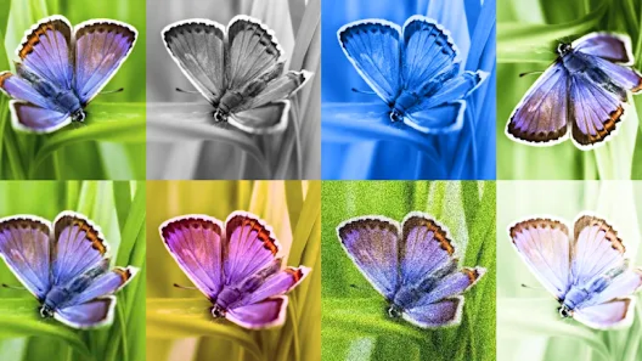
ML systems that can edit, curate or create images or videos can affect anyone exposed to their outputs, shaping or reinforcing the beliefs of viewers around the world. Research to reduce representational harms, such as reinforcing stereotypes or denigrating or erasing groups of people, requires a deep understanding of both the content and the societal context. It hinges on how different observers perceive themselves, their communities, or how others are represented. There’s considerable debate in the field regarding which social categories should be studied with computational tools and how to do so responsibly. Our research focuses on working toward scalable solutions that are informed by sociology and social psychology, are aligned with human perception, embrace the subjective nature of the problem, and enable nuanced measurement and mitigation. One example is our research on differences in human perception and annotation of skin tone in images using the Monk Skin Tone scale.
Our tools are also used to study representation in large-scale content collections. Through our Media Understanding for Social Exploration (MUSE) project, we’ve partnered with academic researchers, nonprofit organizations, and major consumer brands to understand patterns in mainstream media and advertising content. We first published this work in 2017, with a co-authored study analyzing gender equity in Hollywood movies. Since then, we’ve increased the scale and depth of our analyses. In 2019, we released findings based on over 2.7 million YouTube advertisements. In the latest study, we examine representation across intersections of perceived gender presentation, perceived age, and skin tone in over twelve years of popular U.S. television shows. These studies provide insights for content creators and advertisers and further inform our own research.
 |
| An illustration (not actual data) of computational signals that can be analyzed at scale to reveal representational patterns in media collections. [Video Collection / Getty Images] |
Moving forward, we’re expanding the ML fairness concepts on which we focus and the domains in which they are responsibly applied. Looking beyond photorealistic images of people, we are working to develop tools that model the representation of communities and cultures in illustrations, abstract depictions of humanoid characters, and even images with no people in them at all. Finally, we need to reason about not just who is depicted, but how they are portrayed — what narrative is communicated through the surrounding image content, the accompanying text, and the broader cultural context.
Building advanced ML systems is complex, with multiple stakeholders informing various criteria that decide product behavior. Overall quality has historically been defined and measured using summary statistics (like overall accuracy) over a test dataset as a proxy for user experience. But not all users experience products in the same way.
Perception Fairness enables practical measurement of nuanced system behavior beyond summary statistics, and makes these metrics core to the system quality that directly informs product behaviors and launch decisions. This is often much harder than it seems. Distilling complex bias issues (e.g., disparities in performance across intersectional subgroups or instances of stereotype reinforcement) to a small number of metrics without losing important nuance is extremely challenging. Another challenge is balancing the interplay between fairness metrics and other product metrics (e.g., user satisfaction, accuracy, latency), which are often phrased as conflicting despite being compatible. It is common for researchers to describe their work as optimizing an “accuracy-fairness” tradeoff when in reality widespread user satisfaction is aligned with meeting fairness and inclusion objectives.
 |
| We built and released the MIAP dataset as part of Open Images, leveraging our research on perception of socially relevant concepts and detection of biased behavior in complex systems to create a resource that furthers ML fairness research in computer vision. Original photo credits — left: Boston Public Library; middle: jen robinson; right: Garin Fons; all used with permission under the CC- BY 2.0 license. |
To these ends, our team focuses on two broad research directions. First, democratizing access to well-understood and widely-applicable fairness analysis tooling, engaging partner organizations in adopting them into product workflows, and informing leadership across the company in interpreting results. This work includes developing broad benchmarks, curating widely-useful high-quality test datasets and tooling centered around techniques such as sliced analysis and counterfactual testing — often building on the core representation signals work described earlier. Second, advancing novel approaches towards fairness analytics — including partnering with product efforts that may result in breakthrough findings or inform launch strategy.
Our work does not stop with analyzing model behavior. Rather, we use this as a jumping-off point for identifying algorithmic improvements in collaboration with other researchers and engineers on product teams. Over the past year we’ve launched upgraded components that power Search and Memories features in Google Photos, leading to more consistent performance and drastically improving robustness through added layers that keep mistakes from cascading through the system. We are working on improving ranking algorithms in Google Images to diversify representation. We updated algorithms that may reinforce historical stereotypes, using additional signals responsibly, such that it’s more likely for everyone to see themselves reflected in Search results and find what they’re looking for.
This work naturally carries over to the world of generative AI, where models can create collections of images or videos seeded from image and text prompts and can answer questions about images and videos. We’re excited about the potential of these technologies to deliver new experiences to users and as tools to further our own research. To enable this, we’re collaborating across the research and responsible AI communities to develop guardrails that mitigate failure modes. We’re leveraging our tools for understanding representation to power scalable benchmarks that can be combined with human feedback, and investing in research from pre-training through deployment to steer the models to generate higher quality, more inclusive, and more controllable output. We want these models to inspire people, producing diverse outputs, translating concepts without relying on tropes or stereotypes, and providing consistent behaviors and responses across counterfactual variations of prompts.
Despite over a decade of focused work, the field of perception fairness technologies still seems like a nascent and fast-growing space, rife with opportunities for breakthrough techniques. We continue to see opportunities to contribute technical advances backed by interdisciplinary scholarship. The gap between what we can measure in images versus the underlying aspects of human identity and expression is large — closing this gap will require increasingly complex media analytics solutions. Data metrics that indicate true representation, situated in the appropriate context and heeding a diversity of viewpoints, remains an open challenge for us. Can we reach a point where we can reliably identify depictions of nuanced stereotypes, continually update them to reflect an ever-changing society, and discern situations in which they could be offensive? Algorithmic advances driven by human feedback point a promising path forward.
Recent focus on AI safety and ethics in the context of modern large model development has spurred new ways of thinking about measuring systemic biases. We are exploring multiple avenues to use these models — along with recent developments in concept-based explainability methods, causal inference methods, and cutting-edge UX research — to quantify and minimize undesired biased behaviors. We look forward to tackling the challenges ahead and developing technology that is built for everybody.
We would like to thank every member of the Perception Fairness team, and all of our collaborators.