How to compare a noisy quantum processor to a classical computer

How to compare a noisy quantum processor to a classical computer

A full-scale error-corrected quantum computer will be able to solve some problems that are impossible for classical computers, but building such a device is a huge endeavor. We are proud of the milestones that we have achieved toward a fully error-corrected quantum computer, but that large-scale computer is still some number of years away. Meanwhile, we are using our current noisy quantum processors as flexible platforms for quantum experiments.

In contrast to an error-corrected quantum computer, experiments in noisy quantum processors are currently limited to a few thousand quantum operations or gates, before noise degrades the quantum state. In 2019 we implemented a specific computational task called random circuit sampling on our quantum processor and showed for the first time that it outperformed state-of-the-art classical supercomputing.

Although they have not yet reached beyond-classical capabilities, we have also used our processors to observe novel physical phenomena, such as time crystals and Majorana edge modes, and have made new experimental discoveries, such as robust bound states of interacting photons and the noise-resilience of Majorana edge modes of Floquet evolutions.

We expect that even in this intermediate, noisy regime, we will find applications for the quantum processors in which useful quantum experiments can be performed much faster than can be calculated on classical supercomputers — we call these “computational applications” of the quantum processors. No one has yet demonstrated such a beyond-classical computational application. So as we aim to achieve this milestone, the question is: What is the best way to compare a quantum experiment run on such a quantum processor to the computational cost of a classical application?

We already know how to compare an error-corrected quantum algorithm to a classical algorithm. In that case, the field of computational complexity tells us that we can compare their respective computational costs — that is, the number of operations required to accomplish the task. But with our current experimental quantum processors, the situation is not so well defined.

In “Effective quantum volume, fidelity and computational cost of noisy quantum processing experiments”, we provide a framework for measuring the computational cost of a quantum experiment, introducing the experiment’s “effective quantum volume”, which is the number of quantum operations or gates that contribute to a measurement outcome. We apply this framework to evaluate the computational cost of three recent experiments: our random circuit sampling experiment, our experiment measuring quantities known as “out of time order correlators” (OTOCs), and a recent experiment on a Floquet evolution related to the Ising model. We are particularly excited about OTOCs because they provide a direct way to experimentally measure the effective quantum volume of a circuit (a sequence of quantum gates or operations), which is itself a computationally difficult task for a classical computer to estimate precisely. OTOCs are also important in nuclear magnetic resonance and electron spin resonance spectroscopy. Therefore, we believe that OTOC experiments are a promising candidate for a first-ever computational application of quantum processors.

Plot of computational cost and impact of some recent quantum experiments. While some (e.g., QC-QMC 2022) have had high impact and others (e.g., RCS 2023) have had high computational cost, none have yet been both useful and hard enough to be considered a “computational application.” We hypothesize that our future OTOC experiment could be the first to pass this threshold. Other experiments plotted are referenced in the text.

Random circuit sampling: Evaluating the computational cost of a noisy circuit

When it comes to running a quantum circuit on a noisy quantum processor, there are two competing considerations. On one hand, we aim to do something that is difficult to achieve classically. The computational cost — the number of operations required to accomplish the task on a classical computer — depends on the quantum circuit’s effective quantum volume: the larger the volume, the higher the computational cost, and the more a quantum processor can outperform a classical one.

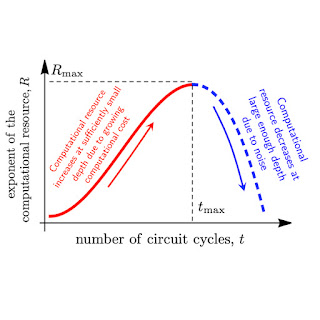
But on the other hand, on a noisy processor, each quantum gate can introduce an error to the calculation. The more operations, the higher the error, and the lower the fidelity of the quantum circuit in measuring a quantity of interest. Under this consideration, we might prefer simpler circuits with a smaller effective volume, but these are easily simulated by classical computers. The balance of these competing considerations, which we want to maximize, is called the “computational resource”, shown below.

Graph of the tradeoff between quantum volume and noise in a quantum circuit, captured in a quantity called the “computational resource.” For a noisy quantum circuit, this will initially increase with the computational cost, but eventually, noise will overrun the circuit and cause it to decrease.

We can see how these competing considerations play out in a simple “hello world” program for quantum processors, known as random circuit sampling (RCS), which was the first demonstration of a quantum processor outperforming a classical computer. Any error in any gate is likely to make this experiment fail. Inevitably, this is a hard experiment to achieve with significant fidelity, and thus it also serves as a benchmark of system fidelity. But it also corresponds to the highest known computational cost achievable by a quantum processor. We recently reported the most powerful RCS experiment performed to date, with a low measured experimental fidelity of 1.7×10⁻³, and a high theoretical computational cost of ~1023. These quantum circuits had 700 two-qubit gates. We estimate that this experiment would take ~47 years to simulate in the world’s largest supercomputer. While this checks one of the two boxes needed for a computational application — it outperforms a classical supercomputer — it is not a particularly useful application per se.

OTOCs and Floquet evolution: The effective quantum volume of a local observable

There are many open questions in quantum many-body physics that are classically intractable, so running some of these experiments on our quantum processor has great potential. We typically think of these experiments a bit differently than we do the RCS experiment. Rather than measuring the quantum state of all qubits at the end of the experiment, we are usually concerned with more specific, local physical observables. Because not every operation in the circuit necessarily impacts the observable, a local observable’s effective quantum volume might be smaller than that of the full circuit needed to run the experiment.

We can understand this by applying the concept of a light cone from relativity, which determines which events in space-time can be causally connected: some events cannot possibly influence one another because information takes time to propagate between them. We say that two such events are outside their respective light cones. In a quantum experiment, we replace the light cone with something called a “butterfly cone,” where the growth of the cone is determined by the butterfly speed — the speed with which information spreads throughout the system. (This speed is characterized by measuring OTOCs, discussed later.) The effective quantum volume of a local observable is essentially the volume of the butterfly cone, including only the quantum operations that are causally connected to the observable. So, the faster information spreads in a system, the larger the effective volume and therefore the harder it is to simulate classically.

A depiction of the effective volume Veff of the gates contributing to the local observable B. A related quantity called the effective area Aeff is represented by the cross-section of the plane and the cone. The perimeter of the base corresponds to the front of information travel that moves with the butterfly velocity vB.

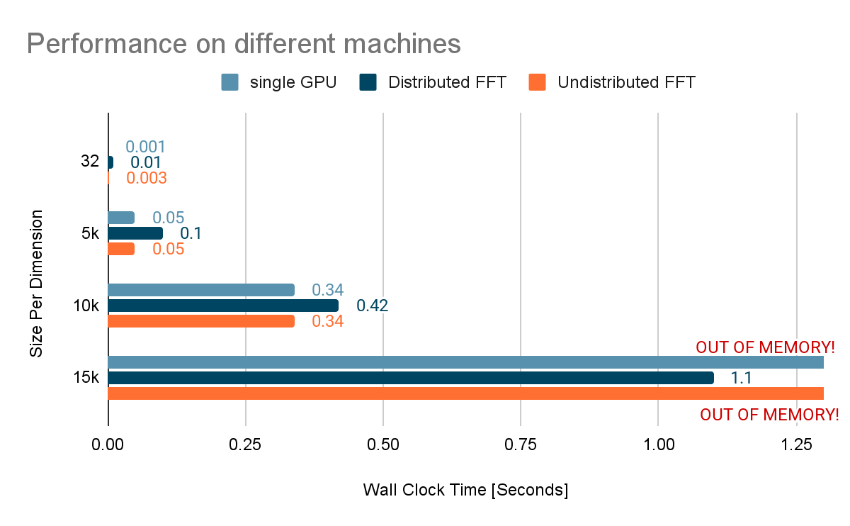
We apply this framework to a recent experiment implementing a so-called Floquet Ising model, a physical model related to the time crystal and Majorana experiments. From the data of this experiment, one can directly estimate an effective fidelity of 0.37 for the largest circuits. With the measured gate error rate of ~1%, this gives an estimated effective volume of ~100. This is much smaller than the light cone, which included two thousand gates on 127 qubits. So, the butterfly velocity of this experiment is quite small. Indeed, we argue that the effective volume covers only ~28 qubits, not 127, using numerical simulations that obtain a larger precision than the experiment. This small effective volume has also been corroborated with the OTOC technique. Although this was a deep circuit, the estimated computational cost is 5×10¹¹, almost one trillion times less than the recent RCS experiment. Correspondingly, this experiment can be simulated in less than a second per data point on a single A100 GPU. So, while this is certainly a useful application, it does not fulfill the second requirement of a computational application: substantially outperforming a classical simulation.

Information scrambling experiments with OTOCs are a promising avenue for a computational application. OTOCs can tell us important physical information about a system, such as the butterfly velocity, which is critical for precisely measuring the effective quantum volume of a circuit. OTOC experiments with fast entangling gates offer a potential path for a first beyond-classical demonstration of a computational application with a quantum processor. Indeed, in our experiment from 2021 we achieved an effective fidelity of Feff ~ 0.06 with an experimental signal-to-noise ratio of ~1, corresponding to an effective volume of ~250 gates and a computational cost of 2×10¹².

While these early OTOC experiments are not sufficiently complex to outperform classical simulations, there is a deep physical reason why OTOC experiments are good candidates for the first demonstration of a computational application. Most of the interesting quantum phenomena accessible to near-term quantum processors that are hard to simulate classically correspond to a quantum circuit exploring many, many quantum energy levels. Such evolutions are typically chaotic and standard time-order correlators (TOC) decay very quickly to a purely random average in this regime. There is no experimental signal left. This does not happen for OTOC measurements, which allows us to grow complexity at will, only limited by the error per gate. We anticipate that a reduction of the error rate by half would double the computational cost, pushing this experiment to the beyond-classical regime.

Conclusion

Using the effective quantum volume framework we have developed, we have determined the computational cost of our RCS and OTOC experiments, as well as a recent Floquet evolution experiment. While none of these meet the requirements yet for a computational application, we expect that with improved error rates, an OTOC experiment will be the first beyond-classical, useful application of a quantum processor.

Read More

Announcing the Preview of Amazon SageMaker Profiler: Track and visualize detailed hardware performance data for your model training workloads

Announcing the Preview of Amazon SageMaker Profiler: Track and visualize detailed hardware performance data for your model training workloads

Today, we’re pleased to announce the preview of Amazon SageMaker Profiler, a capability of Amazon SageMaker that provides a detailed view into the AWS compute resources provisioned during training deep learning models on SageMaker. With SageMaker Profiler, you can track all activities on CPUs and GPUs, such as CPU and GPU utilizations, kernel runs on GPUs, kernel launches on CPUs, sync operations, memory operations across GPUs, latencies between kernel launches and corresponding runs, and data transfer between CPUs and GPUs. In this post, we walk you through the capabilities of SageMaker Profiler.

SageMaker Profiler provides Python modules for annotating PyTorch or TensorFlow training scripts and activating SageMaker Profiler. It also offers a user interface (UI) that visualizes the profile, a statistical summary of profiled events, and the timeline of a training job for tracking and understanding the time relationship of the events between GPUs and CPUs.

The need for profiling training jobs

With the rise of deep learning (DL), machine learning (ML) has become compute and data intensive, typically requiring multi-node, multi-GPU clusters. As state-of-the-art models grow in size in the order of trillions of parameters, their computational complexity and cost also increase rapidly. ML practitioners have to cope with common challenges of efficient resource utilization when training such large models. This is particularly evident in large language models (LLMs), which typically have billions of parameters and therefore require large multi-node GPU clusters in order to train them efficiently.

When training these models on large compute clusters, we can encounter compute resource optimization challenges such as I/O bottlenecks, kernel launch latencies, memory limits, and low resource utilizations. If the training job configuration is not optimized, these challenges can result in inefficient hardware utilization and longer training times or incomplete training runs, which increase the overall costs and timelines for the project.

Prerequisites

The following are the prerequisites to start using SageMaker Profiler:

  • A SageMaker domain in your AWS account – For instructions on setting up a domain, see Onboard to Amazon SageMaker Domain using quick setup. You also need to add domain user profiles for individual users to access the SageMaker Profiler UI application. For more information, see Add and remove SageMaker Domain user profiles.
  • Permissions – The following list is the minimum set of permissions that should be assigned to the execution role for using the SageMaker Profiler UI application:
    • sagemaker:CreateApp
    • sagemaker:DeleteApp
    • sagemaker:DescribeTrainingJob
    • sagemaker:SearchTrainingJobs
    • s3:GetObject
    • s3:ListBucket

Prepare and run a training job with SageMaker Profiler

To start capturing kernel runs on GPUs while the training job is running, modify your training script using the SageMaker Profiler Python modules. Import the library and add the start_profiling() and stop_profiling() methods to define the beginning and the end of profiling. You can also use optional custom annotations to add markers in the training script to visualize hardware activities during particular operations in each step.

There are two approaches that you can take to profile your training scripts with SageMaker Profiler. The first approach is based on profiling full functions; the second approach is based on profiling specific code lines in functions.

To profile by functions, use the context manager smppy.annotate to annotate full functions. The following example script shows how to implement the context manager to wrap the training loop and full functions in each iteration:

import smppy

sm_prof = smppy.SMProfiler.instance()
config = smppy.Config()
config.profiler = {
    "EnableCuda": "1",
}
sm_prof.configure(config)
sm_prof.start_profiling()

for epoch in range(args.epochs):
    if world_size > 1:
        sampler.set_epoch(epoch)
    tstart = time.perf_counter()
    for i, data in enumerate(trainloader, 0):
        with smppy.annotate("step_"+str(i)):
            inputs, labels = data
            inputs = inputs.to("cuda", non_blocking=True)
            labels = labels.to("cuda", non_blocking=True)
    
            optimizer.zero_grad()
    
            with smppy.annotate("Forward"):
                outputs = net(inputs)
            with smppy.annotate("Loss"):
                loss = criterion(outputs, labels)
            with smppy.annotate("Backward"):
                loss.backward()
            with smppy.annotate("Optimizer"):
                optimizer.step()

sm_prof.stop_profiling()

You can also use smppy.annotation_begin() and smppy.annotation_end() to annotate specific lines of code in functions. For more information, refer to documentation.

Configure the SageMaker training job launcher

After you’re done annotating and setting up the profiler initiation modules, save the training script and prepare the SageMaker framework estimator for training using the SageMaker Python SDK.

  1. Set up a profiler_config object using the ProfilerConfig and Profiler modules as follows:
    from sagemaker import ProfilerConfig, Profiler
    profiler_config = ProfilerConfig(
        profiler_params = Profiler(cpu_profiling_duration=3600))

  2. Create a SageMaker estimator with the profiler_config object created in the previous step. The following code shows an example of creating a PyTorch estimator:
    import sagemaker
    from sagemaker.pytorch import PyTorch
    
    estimator = PyTorch(
        framework_version="2.0.0",
        image_uri="763104351884.dkr.ecr.<region>.amazonaws.com/pytorch-training:2.0.0-gpu-py310-cu118-ubuntu20.04-sagemaker",
        role=sagemaker.get_execution_role(),
        entry_point="train_with_profiler_demo.py", # your training job entry point
        source_dir=source_dir, # source dir for your training script
        output_path=output_path,
        base_job_name="sagemaker-profiler-demo",
        hyperparameters=hyperparameters, # if any
        instance_count=1, 
        instance_type=ml.p4d.24xlarge,
        profiler_config=profiler_config
    )

If you want to create a TensorFlow estimator, import sagemaker.tensorflow.TensorFlow instead, and specify one of the TensorFlow versions supported by SageMaker Profiler. For more information about supported frameworks and instance types, see Supported frameworks.

  1. Start the training job by running the fit method:
    estimator.fit(wait=False)

Launch the SageMaker Profiler UI

When the training job is complete, you can launch the SageMaker Profiler UI to visualize and explore the profile of the training job. You can access the SageMaker Profiler UI application through the SageMaker Profiler landing page on the SageMaker console or through the SageMaker domain.

To launch the SageMaker Profiler UI application on the SageMaker console, complete the following steps:

  1. On the SageMaker console, choose Profiler in the navigation pane.
  2. Under Get started, select the domain in which you want to launch the SageMaker Profiler UI application.

If your user profile only belongs to one domain, you will not see the option for selecting a domain.

  1. Select the user profile for which you want to launch the SageMaker Profiler UI application.

If there is no user profile in the domain, choose Create user profile. For more information about creating a new user profile, see Add and Remove User Profiles.

  1. Choose Open Profiler.

You can also launch the SageMaker Profiler UI from the domain details page.

Gain insights from the SageMaker Profiler

When you open the SageMaker Profiler UI, the Select and load a profile page opens, as shown in the following screenshot.

You can view a list of all the training jobs that have been submitted to SageMaker Profiler and search for a particular training job by its name, creation time, and run status (In Progress, Completed, Failed, Stopped, or Stopping). To load a profile, select the training job you want to view and choose Load. The job name should appear in the Loaded profile section at the top.

Choose the job name to generate the dashboard and timeline. Note that when you choose the job, the UI automatically opens the dashboard. You can load and visualize one profile at a time. To load another profile, you must first unload the previously loaded profile. To unload a profile, choose the trash bin icon in the Loaded profile section.

For this post, we view the profile of an ALBEF training job on two ml.p4d.24xlarge instances.

After you finish loading and selecting the training job, the UI opens the Dashboard page, as shown in the following screenshot.

You can see the plots for key metrics, namely the GPU active time, GPU utilization over time, CPU active time, and CPU utilization over time. The GPU active time pie chart shows the percentage of GPU active time vs. GPU idle time, which enables us to check if the GPUs are more active than idle throughout the entire training job. The GPU utilization over time timeline graph shows the average GPU utilization rate over time per node, aggregating all the nodes in a single chart. You can check if the GPUs have an unbalanced workload, under-utilization issues, bottlenecks, or idle issues during certain time intervals. For more details on interpreting these metrics, refer to documentation.

The dashboard provides you with additional plots, including time spent by all GPU kernels, time spent by the top 15 GPU kernels, launch counts of all GPU kernels, and launch counts of the top 15 GPU kernels, as shown in the following screenshot.

Lastly, the dashboard enables you to visualize additional metrics, such as the step time distribution, which is a histogram that shows the distribution of step durations on GPUs, and the kernel precision distribution pie chart, which shows the percentage of time spent on running kernels in different data types such as FP32, FP16, INT32, and INT8.

You can also obtain a pie chart on the GPU activity distribution that shows the percentage of time spent on GPU activities, such as running kernels, memory (memcpy and memset), and synchronization (sync). You can visualize the percentage of time spent on GPU memory operations from the GPU memory operations distribution pie chart.

You can also create your own histograms based on a custom metric that you annotated manually as described earlier in this post. When adding a custom annotation to a new histogram, select or enter the name of the annotation you added in the training script.

Timeline interface

The SageMaker Profiler UI also includes a timeline interface, which provides you with a detailed view into the compute resources at the level of operations and kernels scheduled on the CPUs and run on the GPUs. The timeline is organized in a tree structure, giving you information from the host level to the device level, as shown in the following screenshot.

For each CPU, you can track the CPU performance counters, such as clk_unhalted_ref.tsc and itlb_misses.miss_causes_a_walk. For each GPU on the 2x p4d.24xlarge instance, you can see a host timeline and a device timeline. Kernel launches are on the host timeline and kernel runs are on the device timeline.

You can also zoom in to the individual steps. In the following screenshot, we have zoomed in to step_41. The timeline strip selected in the following screenshot is the AllReduce operation, an essential communication and synchronization step in distributed training, run on GPU-0. In the screenshot, note that the kernel launch in the GPU-0 host connects to the kernel run in the GPU-0 device stream 1, indicated with the arrow in cyan.

Availability and considerations

SageMaker Profiler is available in PyTorch (version 2.0.0 and 1.13.1) and TensorFlow (version 2.12.0 and 2.11.1). The following table provides the links to the supported AWS Deep Learning Containers for SageMaker.

Framework Version AWS DLC Image URI
PyTorch 2.0.0 763104351884.dkr.ecr.<region>.amazonaws.com/pytorch-training:2.0.0-gpu-py310-cu118-ubuntu20.04-sagemaker
PyTorch 1.13.1 763104351884.dkr.ecr.<region>.amazonaws.com/pytorch-training:1.13.1-gpu-py39-cu117-ubuntu20.04-sagemaker
TensorFlow 2.12.0 763104351884.dkr.ecr.<region>.amazonaws.com/tensorflow-training:2.12.0-gpu-py310-cu118-ubuntu20.04-sagemaker
TensorFlow 2.11.1 763104351884.dkr.ecr.<region>.amazonaws.com/tensorflow-training:2.11.1-gpu-py39-cu112-ubuntu20.04-sagemaker

SageMaker Profiler is currently available in the following Regions: US East (Ohio, N. Virginia), US West (Oregon), and Europe (Frankfurt, Ireland).

SageMaker Profiler is available in the training instance types ml.p4d.24xlarge, ml.p3dn.24xlarge, and ml.g4dn.12xlarge.

For the full list of supported frameworks and versions, refer to documentation.

SageMaker Profiler incurs charges after the SageMaker Free Tier or the free trial period of the feature ends. For more information, see Amazon SageMaker Pricing.

Performance of SageMaker Profiler

We compared the overhead of SageMaker Profiler against various open-source profilers. The baseline used for the comparison was obtained from running the training job without a profiler.

Our key finding revealed that SageMaker Profiler generally resulted in a shorter billable training duration because it had less overhead time on the end-to-end training runs. It also generated less profiling data (up to 10 times less) when compared against open-source alternatives. The smaller profiling artifacts generated by SageMaker Profiler require less storage, thereby also saving on costs.

Conclusion

SageMaker Profiler enables you to get detailed insights into the utilization of compute resources when training your deep learning models. This can enable you to resolve performance hotspots and bottlenecks to ensure efficient resource utilization that would ultimately drive down training costs and reduce the overall training duration.

To get started with SageMaker Profiler, refer to documentation.


About the Authors

 Roy Allela is a Senior AI/ML Specialist Solutions Architect at AWS based in Munich, Germany. Roy helps AWS customers—from small startups to large enterprises—train and deploy large language models efficiently on AWS. Roy is passionate about computational optimization problems and improving the performance of AI workloads.

Sushant Moon is a Data Scientist at AWS, India, specializing in guiding customers through their AI/ML endeavors. With a diverse background spanning retail, finance, and insurance domains, he delivers innovative and tailored solutions. Beyond his professional life, Sushant finds rejuvenation in swimming and seeks inspiration from his travels to diverse locales.

Diksha Sharma is an AI/ML Specialist Solutions Architect in the Worldwide Specialist Organization. She works with public sector customers to help them architect efficient, secure, and scalable machine learning applications including generative AI solutions on AWS. In her spare time, Diksha loves to read, paint, and spend time with her family.

Read More

Teaching language models to reason algorithmically

Teaching language models to reason algorithmically

Large language models (LLMs), such as GPT-3 and PaLM, have shown impressive progress in recent years, which have been driven by scaling up models and training data sizes. Nonetheless, a long standing debate has been whether LLMs can reason symbolically (i.e., manipulating symbols based on logical rules). For example, LLMs are able to perform simple arithmetic operations when numbers are small, but struggle to perform with large numbers. This suggests that LLMs have not learned the underlying rules needed to perform these arithmetic operations.

While neural networks have powerful pattern matching capabilities, they are prone to overfitting to spurious statistical patterns in the data. This does not hinder good performance when the training data is large and diverse and the evaluation is in-distribution. However, for tasks that require rule-based reasoning (such as addition), LLMs struggle with out-of-distribution generalization as spurious correlations in the training data are often much easier to exploit than the true rule-based solution. As a result, despite significant progress in a variety of natural language processing tasks, performance on simple arithmetic tasks like addition has remained a challenge. Even with modest improvement of GPT-4 on the MATH dataset, errors are still largely due to arithmetic and calculation mistakes. Thus, an important question is whether LLMs are capable of algorithmic reasoning, which involves solving a task by applying a set of abstract rules that define the algorithm.

In “Teaching Algorithmic Reasoning via In-Context Learning”, we describe an approach that leverages in-context learning to enable algorithmic reasoning capabilities in LLMs. In-context learning refers to a model’s ability to perform a task after seeing a few examples of it within the context of the model. The task is specified to the model using a prompt, without the need for weight updates. We also present a novel algorithmic prompting technique that enables general purpose language models to achieve strong generalization on arithmetic problems that are more difficult than those seen in the prompt. Finally, we demonstrate that a model can reliably execute algorithms on out-of-distribution examples with an appropriate choice of prompting strategy.

By providing algorithmic prompts, we can teach a model the rules of arithmetic via in-context learning. In this example, the LLM (word predictor) outputs the correct answer when prompted with an easy addition question (e.g., 267+197), but fails when asked a similar addition question with longer digits. However, when the more difficult question is appended with an algorithmic prompt for addition (blue box with white + shown below the word predictor), the model is able to answer correctly. Moreover, the model is capable of simulating the multiplication algorithm (X) by composing a series of addition calculations.

Teaching an algorithm as a skill

In order to teach a model an algorithm as a skill, we develop algorithmic prompting, which builds upon other rationale-augmented approaches (e.g., scratchpad and chain-of-thought). Algorithmic prompting extracts algorithmic reasoning abilities from LLMs, and has two notable distinctions compared to other prompting approaches: (1) it solves tasks by outputting the steps needed for an algorithmic solution, and (2) it explains each algorithmic step with sufficient detail so there is no room for misinterpretation by the LLM.

To gain intuition for algorithmic prompting, let’s consider the task of two-number addition. In a scratchpad-style prompt, we process each digit from right to left and keep track of the carry value (i.e., we add a 1 to the next digit if the current digit is greater than 9) at each step. However, the rule of carry is ambiguous after seeing only a few examples of carry values. We find that including explicit equations to describe the rule of carry helps the model focus on the relevant details and interpret the prompt more accurately. We use this insight to develop an algorithmic prompt for two-number addition, where we provide explicit equations for each step of computation and describe various indexing operations in non-ambiguous formats.

Illustration of various prompt strategies for addition.

Using only three prompt examples of addition with answer length up to five digits, we evaluate performance on additions of up to 19 digits. Accuracy is measured over 2,000 total examples sampled uniformly over the length of the answer. As shown below, the use of algorithmic prompts maintains high accuracy for questions significantly longer than what’s seen in the prompt, which demonstrates that the model is indeed solving the task by executing an input-agnostic algorithm.

Test accuracy on addition questions of increasing length for different prompting methods.

Leveraging algorithmic skills as tool use

To evaluate if the model can leverage algorithmic reasoning in a broader reasoning process, we evaluate performance using grade school math word problems (GSM8k). We specifically attempt to replace addition calculations from GSM8k with an algorithmic solution.

Motivated by context length limitations and possible interference between different algorithms, we explore a strategy where differently-prompted models interact with one another to solve complex tasks. In the context of GSM8k, we have one model that specializes in informal mathematical reasoning using chain-of-thought prompting, and a second model that specializes in addition using algorithmic prompting. The informal mathematical reasoning model is prompted to output specialized tokens in order to call on the addition-prompted model to perform the arithmetic steps. We extract the queries between tokens, send them to the addition-model and return the answer to the first model, after which the first model continues its output. We evaluate our approach using a difficult problem from the GSM8k (GSM8k-Hard), where we randomly select 50 addition-only questions and increase the numerical values in the questions.

An example from the GSM8k-Hard dataset. The chain-of-thought prompt is augmented with brackets to indicate when an algorithmic call should be performed.

We find that using separate contexts and models with specialized prompts is an effective way to tackle GSM8k-Hard. Below, we observe that the performance of the model with algorithmic call for addition is 2.3x the chain-of-thought baseline. Finally, this strategy presents an example of solving complex tasks by facilitating interactions between LLMs specialized to different skills via in-context learning.

Chain-of-thought (CoT) performance on GSM8k-Hard with or without algorithmic call.

Conclusion

We present an approach that leverages in-context learning and a novel algorithmic prompting technique to unlock algorithmic reasoning abilities in LLMs. Our results suggest that it may be possible to transform longer context into better reasoning performance by providing more detailed explanations. Thus, these findings point to the ability of using or otherwise simulating long contexts and generating more informative rationales as promising research directions.

Acknowledgements

We thank our co-authors Behnam Neyshabur, Azade Nova, Hugo Larochelle and Aaron Courville for their valuable contributions to the paper and great feedback on the blog. We thank Tom Small for creating the animations in this post. This work was done during Hattie Zhou’s internship at Google Research.

Read More

Distributed Fast Fourier Transform in TensorFlow

Distributed Fast Fourier Transform in TensorFlow

Posted by Ruijiao Sun, Google Intern – DTensor team

Fast Fourier Transform is an important method of signal processing, which is commonly used in a number of ways, including speeding up convolutions, extracting features, and regularizing models. Distributed Fast Fourier Transform (Distributed FFT) offers a way to compute Fourier Transforms in models that work with image-like datasets that are too large to fit into the memory of a single accelerator device. In a previous Google Research Paper, “Large-Scale Discrete Fourier Transform on TPUs” by Tianjian Lu, a Distributed FFT algorithm was implemented for TensorFlow v1 as a library. This work presents the newly added native support in TensorFlow v2 for Distributed FFT, through the new TensorFlow distribution API, DTensor.

About DTensor

DTensor is an extension to TensorFlow for synchronous distributed computing. It distributes the program and tensors through a procedure called Single program, multiple data (SPMD) extension. DTensor offers an uniform API for traditional data and model parallelism patterns used widely in Machine Learning.

Example Usage

The API interface for distributed FFT is the same as the original FFT in TensorFlow. Users just need to pass a sharded tensor as an input to the existing FFT ops in TensorFlow, such as tf.signal.fft2d. The output of a distributed FFT becomes sharded too.

import TensorFlow as tf
from TensorFlow.experimental import dtensor

# Set up devices
device_type = dtensor.preferred_device_type()
if device_type == 'CPU':
cpu = tf.config.list_physical_devices(device_type)
tf.config.set_logical_device_configuration(cpu[0], [tf.config.LogicalDeviceConfiguration()] * 8)
if device_type == 'GPU':
gpu = tf.config.list_physical_devices(device_type)
tf.config.set_logical_device_configuration(gpu[0], [tf.config.LogicalDeviceConfiguration(memory_limit=1000)] * 8)
dtensor.initialize_accelerator_system()

# Create a mesh
mesh = dtensor.create_distributed_mesh(mesh_dims=[('x', 1), ('y', 2), ('z', 4)], device_type=device_type)

# Set up a distributed input Tensor
input = tf.complex(
tf.random.stateless_normal(shape=(2, 2, 4), seed=(1, 2), dtype=tf.float32),
tf.random.stateless_normal(shape=(2, 2, 4), seed=(2, 4), dtype=tf.float32))
init_layout = dtensor.Layout(['x', 'y', 'z'], mesh)
d_input = dtensor.relayout(input, layout=init_layout)

# Run distributed fft2d. DTensor determines the most efficient
#
layout of of d_output.
d_output = tf.signal.fft2d(d_input)

Performance Analysis

The following experiment demonstrates that the distributed FFT can process more data than the non-distributed one by utilizing memory across multiple devices. The tradeoff is spending additional time on communication and data transposes that slow down the calculation speed.

Graph of performance on different machines, measuri8ng wall clock time in seconds by size per dimension across single GPU, Distributed FFT and Undistributed FFT

This phenomenon is shown in detail from the profiling result of the 10K*10K distributed FFT experiment. The current implementation of distributed FFT in TensorFlow follows the simple shuffle+local FFT method, which is also used by other popular distributed FFT libraries such as FFTW and PFFT. Notably, the two local FFT ops only take 3.6% of the total time (15ms). This is around 1/3 of the time for non-distributed fft2d. Most of the computing time is spent on data shuffling, represented by the ncclAllToAll Operation. Note that these experiments were conducted on an 8xV100 GPU system.

Table of Top 10 TensorFlow operations on GPU highlighting two local FFT ops in the top 3

Next steps

The feature is new and we have adopted a simplest distributed FFT algorithm. A few ideas to fine tune or improve the performance are:

  • Switch to a different DFT/FFT algorithm.
  • Tweaks on the NCCL communication settings for the particular FFT sizes may improve utilization of the network bandwidth and increase the speed.
  • Reducing the number of collectives to minimize bandwidth requirements.
  • Use N-d local FFTs, rather than multiple 1-d local FFTs.

Try the new distributed FFT! We welcome your feedback on the TensorFlow Forum and look forward to working with you on improving the performance. Your input would be invaluable!

Read More

Xbox PC Game Pass Comes to GeForce NOW, Along With 25 New Games

Xbox PC Game Pass Comes to GeForce NOW, Along With 25 New Games

As part of NVIDIA and Microsoft’s collaboration to bring more choice to gamers, new Microsoft Store integration has been added to GeForce NOW that lets gamers stream select titles from the Xbox PC Game Pass catalog on GeForce NOW, starting today.

With the Microsoft Store integration, members will see a brand-new Xbox button on supported PC games and can seamlessly launch these titles across their devices, provided they either purchased the standalone games through the Microsoft Store or have an active Xbox Game Pass Ultimate or PC Game Pass subscription.

Hot off our recent Gamescom announcement, four blockbuster titles are coming to GeForce NOW this fall: Alan Wake 2, Cyberpunk 2077: Phantom Liberty expansion, Party Animals and PAYDAY 3.

Plus, head to the cloud and stream the 25 new titles joining the cloud this week, including DOOM 2016 from Bethesda.

Members have also been playing the GeForce NOW Ultimate KovaaK’s challenge, raising the bar with 240 frames per second streaming using an Ultimate membership. Check out the leaderboard to see how Ultimate members are stacking up against other GeForce NOW members — top scorers have a chance to win some ultimate prizes through Thursday, Sept. 21, including a six-month Xbox PC Game Pass.

Select PC Game Pass Titles Now Available

Xbox PC Game Pass on GeForce NOW
Hello, Xbox.

Give a warm welcome to the Microsoft Store on GeForce NOW. It joins digital platforms Steam, Epic Games Store, Ubisoft Connect and others in the cloud. Experience it today with hit Xbox PC games from Xbox Game Studios, Bethesda and other top publishers recently added to GeForce NOW,  like Fatshark, Paradox and TaleWorld Entertainment.

With a GeForce NOW Ultimate membership, stream popular shooters Gears 5 and Deathloop with the highest graphical fidelity. Embark on a mini-adventure on the big screen by shrinking to the size of an ant in Grounded. Or enjoy the historical narrative Pentiment while on the go with a mobile device.

Take a deep dive into history with titles from the Age of Empires series on a Chromebook and a comfy throne of your own or experience an alternative version of history in the newly added Wolfenstein II: New Colossus and Wolfenstein: Youngblood titles with the power of 4K streaming on NVIDIA SHIELD.

Warhammer 40k: Darktide Xbox PC Game Pass on GeForce NOW
Fight the dark tide with the power of the cloud.

Lead armies in TaleWorld Entertainment’s action role-playing game Mount & Blade II: Bannerlord, take on hordes of enemies in Fatshark’s action shooter Warhammer 40,000: Darktide or explore infinite worlds in Hello Game’s No Man’s Sky. 

Keep an eye out for more games from Xbox’s PC Game Pass library to be added to GeForce NOW. Check out this article for more details on how Xbox PC Game Pass will work on GeForce NOW.

And this week only, on top of being able to win a six-month Ultimate membership and $100 Steam gift card for making it into the top three on the weekly leaderboard of the Ultimate KovaaK’s challenge, those who make it into the top 10 will get a six-month Xbox PC Game Pass. Keep an eye out on GeForce NOW’s Twitter and Facebook accounts for more details.

Straight Out of Gamescom

Top publishers Epic Games Publishing, CD Projekt Red and Deep Silver are all bringing their blockbuster titles to GeForce NOW at launch in the fall.

Alan Wake 2 coming to GeForce NOW
Wake up, it’s the second game in the “Alan Wake” franchise.

Uncover the newest mystery in the upcoming survival horror game Alan Wake 2, sequel to the award-winning game Alan Wake, from Remedy Entertainment and Epic Games Publishing. Survive as the best-selling horror writer Alan Wake — who’s trapped in a dark dimension and trying to write his way out — or as FBI agent Saga Anderson in a life-or-death race to solve a small-town murder that quickly spirals into a nightmare.

Play through two distinct stories set in two beautiful yet terrifying worlds and see events unfold from different perspectives. The characters must take on powerful supernatural enemies and use more than just a gun to survive: light is the ultimate weapon in the fight against darkness. Members can stream the game from the cloud when it launches on Tuesday, Oct. 27.

Cyberpunk 2077 expansion coming to GeForce NOW
Welcome to the neon cloud.

Return as cyber-enhanced mercenary V in the upcoming spy-thriller expansion for the hit open-world action adventure Cyberpunk 2077 from CD Projekt Red. Phantom Liberty features the all-new district of Dogtown, infinitely replayable open-world activities, an exclusive skill tree and much more — including  new weapons, cyberware, vehicles and gigs for players to discover. Embark on a high-stakes mission of espionage and intrigue to save the NUS President when the expansion launches in the cloud on Tuesday, Sept. 26.

PAYDAY 2 coming to GeForce NOW
It pays to be a GeForce NOW member.

Join the Payday Gang in the upcoming third installment of the PAYDAY franchise from Starbeeze Studios, Overkill Software and Deep Silver. In PAYDAY 3, play as notorious criminals who must face off against new enemies and challenges in an action-packed, high-octane experience. Invite your friends to the four-player online co-op mode to pull off the ultimate heist when the title launches on GeForce NOW on Thursday, Sept. 21.

These games are all headed to the cloud this fall. Upgrade to an Ultimate membership today to skip the waiting lines over free members and get access to powerful NVIDIA technology, including RTX ON and DLSS 3.5 technology for AI-powered graphics and peak-performance gaming.

Welcome to the Cloud

DOOM 2016 on GeForce NOW
You won’t be able to resist the power of the cloud.

The next Bethesda game to heat up the cloud is DOOM 2016. Fight through hordes of demonic forces on Mars after waking up on a Union Aerospace Corporation energy-mining facility. Play as the Doom Slayer, an unnamed space marine from the DOOM franchise, and use a variety of weapons, gadgets and melee attacks in this fast-paced, first-person shooter. Plus, several online multiplayer modes are available, so members can grab some buddies to stream with.

Catch the full list of games joining the cloud this week:

  • WrestleQuest (New release on Steam, Aug. 21)
  • Jumplight Odyssey (New release on Steam, Aug. 21)
  • Blasphemous 2 (New release on Steam, Aug. 24)
  • RIDE 5 (New release on Steam, Aug. 24)
  • Age of Empires: Definitive Edition (Xbox)
  • Age of Empires III: Definitive Edition (Xbox)
  • Age of Empires IV: Anniversary Edition (Xbox)
  • Crusader Kings III (Xbox)
  • Dead Cells (Xbox)
  • Deathloop (Xbox)
  • Doom 2016 (Steam)
  • Gears 5 (Xbox)
  • Grounded (Xbox)
  • Mount & Blade II: Bannerlord (Xbox)
  • No Man’s Sky (Xbox)
  • Pentiment (Xbox)
  • Quake (Xbox)
  • Shadowrun: Dragonfall – Director’s Cut (Xbox)
  • Stellaris (Xbox)
  • The Texas Chain Saw Massacre (Xbox)
  • Trackmania (Steam)
  • Valheim (Xbox)
  • Warhammer 40,000: Darktide (Xbox)
  • Wolfenstein: Youngblood (Xbox)
  • Wolfenstein II: The New Colossus (Xbox)

This week’s Game On giveaway with SteelSeries includes Destiny 2 and three-day Priority membership codes. Check the giveaway page for details on how to enter.

What games are you looking forward to? Let us know on Twitter or in the comments below.

Read More

Large Scale Training of Hugging Face Transformers on TPUs With PyTorch/XLA FSDP

Large Scale Training of Hugging Face Transformers on TPUs With PyTorch/XLA FSDP

AI is transforming many industries through advanced capabilities such as understanding and generating language, answering questions, and delivering accurate recommendations. These capabilities are fueled by ever-increasing size and complexity of AI models, which require vast amounts of computing power to train.

To meet the growing demands of AI training at scale, last year we introduced Fully Sharded Data Parallel (FSDP) in PyTorch/XLA. FSDP is a model parallelism architecture that unlocks the ability to easily and efficiently scale AI models into hundreds of billions of parameters. With PyTorch/XLA FSDP, during distributed training, each device can store a specific model shard, and all-gather the full model weights when it is time to perform the forward pass. Nested FSDP further optimizes performance by only using a given layer’s full parameters during its forward pass.

We are excited to announce that PyTorch/XLA FSDP has landed in Hugging Face Transformers. Now, Hugging Face users can train PyTorch models with up to 20 times more parameters using the same amount of computing power as before.

We built PyTorch/XLA FSDP support directly into the Hugging Face Trainer class, so that any model using Trainer can leverage FSDP. And with the addition of automatic wrapping to PyTorch/XLA FSDP, nested FSDP wrapping is both flexible and simple to apply. These new features make it easy to train a wide range of Hugging Face models at large scales. In this guide, we demonstrate training GPT-2 models with up to 128B parameters on Google Cloud TPUs. PyTorch/XLA FSDP training on TPUs is highly efficient, achieving up to 45.1% model FLOPS utilization (MFU) for GPT-2:

Figure 1: Model FLOPS utilization for Hugging Face GPT-2 on Google Cloud TPU v4

Figure 1: Model FLOPS utilization for Hugging Face GPT-2 on Google Cloud TPU v4

Configuring PyTorch/XLA FSDP in the Hugging Face Trainer

First, follow your preferred method to create your TPU(s) and install PyTorch and PyTorch/XLA. You need versions >= 2.0 for PyTorch and PyTorch/XLA.

Unset

pip3 install https://storage.googleapis.com/tpu-pytorch/wheels/tpuvm/torc h-2.0-cp38-cp38-linux_x86_64.whl --user

pip3 install https://storage.googleapis.com/tpu-pytorch/wheels/tpuvm/torc h_xla-2.0-cp38-cp38-linux_x86_64.whl

Next, clone and install the Hugging Face Transformers repo. Install all necessary dependencies (e.g., datasets, evaluate, scikit-learn, accelerate).

Unset

cd $HOME

git clone https://github.com/huggingface/transformers.git cd transformers

git checkout v4.31-release

pip3 install -e .

pip3 install datasets evaluate scikit-learn

pip3 install accelerate==0.21.0

In $HOME/transformers, create any model-specific configuration files you might need. Here is an example of a configuration file for a GPT-2 model with 2B parameters, which we later refer to as gpt2_config.json:

Unset

{

"activation_function": "gelu_new", "architectures": [

"GPT2LMHeadModel"

],

"attn_pdrop": 0.1,

"bos_token_id": 50256, "embd_pdrop": 0.1, "eos_token_id": 50256, "initializer_range": 0.02, "layer_norm_epsilon": 1e-05, "model_type": "gpt2",

"n_embd": 3072,

"n_head": 24,

"n_layer": 18,

"n_positions": 1024, "resid_pdrop": 0.1, "summary_activation": null, "summary_first_dropout": 0.1, "summary_proj_to_labels": true, "summary_type": "cls_index", "summary_use_proj": true,

"task_specific_params": { "text-generation":![ref1] { "do_sample": true, "max_length": 50

}

},

"vocab_size": 50257

}

With PyTorch/XLA FSDP, it is possible to train model sizes much bigger than this on large accelerator slices. We have trained GPT-2 models as large as 128B parameters with these techniques; for expert tips on how to replicate this scale, see the appendix.

In $HOME/transformers, create your FSDP configuration file, a JSON file containing all of the configurable aspects of your XLA FSDP wrapping stored as a dictionary. Following the official Hugging Face Transformers XLA FSDP documentation, the following arguments are available to set:

  • xla (bool, *optional*, defaults to False): This is a boolean which determines whether or not you use XLA FSDP. Make sure to set this to true.
  • xla_fsdp_settings (dict, *optional*): This is a dictionary which stores all of the XLA FSDP wrapping parameters you want to set; note that you do not have to specify settings for parameters where you are using the default value. For a complete list of settings, see here.

For compute_dtype and buffer_dtype, enter these as strings which contain the corresponding torch data type, e.g. bfloat16.

  • fsdp_min_num_params (int, *optional*, defaults to 0): An integer which sets the minimum number of parameters for size-based auto wrapping. Every module with at least as many parameters as fsdp_min_num_params will be XLA FSDP wrapped.
  • fsdp_transformer_layer_cls_to_wrap (List[str], *optional*): A list of (case-sensitive) transformer layer class names to wrap. Note that this is mutually exclusive with fsdp_min_num_params. Example: ["GPT2Block", "GPT2MLP"].
  • xla_fsdp_grad_ckpt (bool, *optional*, defaults to False): This is a boolean which determines whether to use gradient checkpointing over each nested XLA FSDP wrapped layer. This setting can only be used when the xla flag is set to true, and an auto wrapping policy is specified through fsdp_min_num_params or fsdp_transformer_layer_cls_to_wrap.

Note: For transformer-based models, use fsdp_transformer_layer_cls_to_wrap instead of fsdp_min_num_params when performing automatic nested FSDP wrapping. Layers which share weights should not belong to separate FSDP wrapped units, and the input and output embedding layers in transformer-based models share weights.

For this GPT-2 example, here is what the corresponding fsdp_config.json file looks like:

Unset

{
  "fsdp_transformer_layer_cls_to_wrap": [
    "GPT2Block"
  ],
  "xla": true,
  "xla_fsdp_settings": {
    "compute_dtype": "bfloat16",
    "shard_param_on_dim_0": true,
    "pin_layout_in_collective_ops": true
},
       "xla_fsdp_grad_ckpt": true
     }
Now, it’s time to train your model! First, ensure that you have your PyTorch/XLA runtime set up appropriately by setting
Unset
  export PJRT_DEVICE=TPU

When running training, the key flags to pass are:

a) --fsdp "full_shard"
b) --fsdp_config fsdp_config.json

where you should replace fsdp_config.json with whatever you named your FSDP configuration file. Here is a sample command to train our example 2B GPT-2 model, where training is started by xla_spawn.py, a launcher script for distributed TPU training.

Unset

python3 -u examples/pytorch/xla_spawn.py --num_cores 4 examples/pytorch/language-modeling/run_clm.py  --num_train_epochs 1 

--dataset_name wikitext 

--dataset_config_name wikitext-2-raw-v1  --per_device_train_batch_size 32  --per_device_eval_batch_size 32 

--do_train 

--do_eval 

--output_dir /tmp/test-clm 

--overwrite_output_dir 

--config_name gpt2_config.json 

--cache_dir /tmp 

--tokenizer_name gpt2 

--block_size 1024 

--optim adafactor 

--adafactor true 

--save_strategy no 

--logging_strategy no 

--fsdp "full_shard" 

--fsdp_config fsdp_config.json

Measuring Model FLOPS Utilization (MFU) for GPT-2

Model FLOPS are the floating point operations required to perform a single forward and backward pass. Model FLOPS are hardware- and implementation- independent, and only depend on the underlying model. In each step, the number of FLOPS is computed via the following formulas:

Unset

tokens_per_batch = global_batch_size * seq_len

FLOPS_per_step = 6 * tokens_per_batch * num_params

where seq_len is the sequence length and num_params is the number of parameters in the model. We note that this estimation assumes that d_model » sequence length. If this assumption is violated the self-attention FLOPs start to be significant enough and this expression.

Based on the step time and the hardware details (numbers of chips and the peak FLOPS per chip), we can compute Model FLOPS Utilization (MFU), which measures how effectively our implementation is using the underlying hardware. Achieving 100% MFU means that the hardware is being used perfectly by that model. We calculate MFU using the following formula:

Unset

model_FLOPS_utilization = FLOPS_per_step / step_time(s) / chip_count / FLOPS_per_chip

When training a GPT-2 model with 2B parameters with the XLA FSDP configuration file above on a Cloud TPU v4-8, we measure a step time of 4.191s. Using the above formula, we calculate 35.7% MFU on a v4-8. For further details on calculating MFU, refer to the PaLM paper.

The table below presents MFU for GPT-2 models with sizes between 2B and 128B, with a sequence length of 1024.

TPU NumCores v4-8 v4-64 v4-128 v4-128 v4-256 v4-512
# of Tokens / Batch 131,072 524,288 524,288 524,288 1,048,576 1,048,576
# of Parameters 2B 16B 20B 32B 64B 128B
Step Time (ms) 4,191 14,592 7,824 12,970 25,653 30,460
PFLOPS / Step 1.65 50 62 101 404 809
MFU 35.7% 38.8% 45.1% 44.4% 44.7% 37.7%

Table 1: GPT-2 model FLOPS utilization calculation details

Among these configurations, MFU peaks at 45.1% for the 20B parameter model on v4-128. This result compares favorably to, for example, 41.5% MFU for a 22B Megatron-like model.

There are two actionable insights from these experiments:

First, simply increasing the number of chips without increasing the batch size generally means lower FLOPS utilization, because more time is spent on sharing the model shards. FSDP uses all-reduce communication collectives which are not asynchronous, which means that chip-to-chip communication cannot be overlapped with computation. As the number of chips increases, the number of model shards that must be communicated increases, and so we should expect the portion of the step time spent on communication to increase with the number of chips.

Second, increasing the batch size generally means better FLOPS utilization. As the number of chips increases, the memory footprint of the model decreases, which often frees up high bandwidth memory (HBM) to scale up the global batch size. With a larger global batch size, the number of tokens processed in each step increases, and thus, so does the FLOPS per step. As long as the step time does not increase proportionally, we expect a larger global batch size to improve MFU.

Therefore, to maximize the MFU, we recommend training with the largest global batch size possible that can fit in the HBM of the TPU slice, using FSDP to reduce memory required for the model parameters.

Training Very Large Models (tested to 128B parameters)

When using PyTorch/XLA, tensors must be initialized on the CPU before being moved to the XLA device. This means one may encounter host-side out-of-memory errors if the model is sufficiently large, even though the model can fit in the device HBM after sharding. To avoid this, we must defer each submodule’s initialization until it is FSDP wrapped, which ensures that submodules are sharded as soon as their values are populated, avoiding host-side limitations.

Below, we explain how to modify a local copy of the Hugging Face transformers repository to train a GPT-2 model with up to 128B parameters using this technique.

First, using the commands below, install torchdistX, which is a library containing experimental PyTorch Distributed features. This is the engine behind deferred initialization, and allows you to create tensors that don’t require immediate storage and can be materialized later. You also need to install a specific PyTorch/XLA 2.0 version that takes advantage of this package; note that you must uninstall PyTorch and PyTorch/XLA first, if you installed them earlier.

Unset

pip3 install torch==2.0 --index-url [https://download.pytorch.org/whl/test/cpu --user](https://download.pytorch.org/whl/test/cpu)

pip3 install torch_xla[torchdistx] -f https://storage.googleapis.com/tpu-pytorch/wheels/tpuvm/experimen tal/torch_xla-2.0-cp38-cp38-linux_x86_64.whl

Next, apply the following changes to your local copy of Hugging Face Transformers:

In src/transformers/trainer.py, add the following function in _wrap_model on the line immediately prior to PyTorch/XLA FSDP wrapping:

Python

from torchdistx import deferred_init

def _init_with_torchdistX(module):

def check_fn(k):

return not isinstance(k, FSDP) deferred_init.materialize_module(module, check_fn=check_fn)

The function materialize_module will initialize the model tensors if check_fn returns True. In this case, check_fn checks whether the module has been FSDP wrapped.

Within _wrap_model, modify your FSDP wrapping to accept the additional argument param_init_fn=_init_with_torchdistX:

Python

self.model = model = FSDP(

model,

auto_wrap_policy=auto_wrap_policy, auto_wrapper_callable=auto_wrapper_callable, param_init_fn=_init_with_torchdistX, **fsdp_kwargs,

)

In examples/pytorch/language-modeling/run_clm.py, add the following import statement at the beginning of the file:

Python

from torchdistx import deferred_init

Edit the model initialization so that the model is wrapped with deferred_init.deferred_init by replacing the line

Python

model = AutoModelForCausalLM.from_config(config)

with

Python

model = deferred_init.deferred_init(AutoModelForCausalLM.from_config, config)

Note that this assumes you are supplying your own model configuration file. Otherwise, you should modify your model initialization statement accordingly.

You should also comment out these two lines which immediately follow the line above:

Python

n_params = sum({p.data_ptr(): p.numel() for p in model.parameters()}.values()) logger.info(f"Training new model from scratch - Total size={n_params/2**20:.2f}M params")

They will cause an error if left unmodified, since the model tensors do not actually have storage when these lines are executed.

With these changes, you can now run GPT-2 models with as many as 128B parameters, provided the accelerator size is suitably large.

Next Steps & Acknowledgements

To learn more, the docs can be found here. We’d love to hear from you if you run into any issues with FSDP in PyTorch/XLA, or just want to tell us about how you are using it.

We are ecstatic about what’s ahead for PyTorch/XLA and invite the community to join us. PyTorch/XLA is developed fully in open source. So, please file issues, submit pull requests, and send RFCs to GitHub so that we can openly collaborate.

We’d like to thank Ronghang Hu and Ross Girshick at Meta AI and Lysandre Debut, Sourab Mangrulkar, Sylvain Gugger and Arthur Zucker for all the support and collaboration. We’d also like to thank Jiewen Tan, Liyang Lu, Will Cromar, Vaibhav Singh, and Chandra Devarakonda for their assistance in preparing this post.

Cheers!

The PyTorch/XLA Team at Google

Read More

Persistent Systems shapes the future of software engineering with Amazon CodeWhisperer

Persistent Systems shapes the future of software engineering with Amazon CodeWhisperer

Amazon CodeWhisperer, the AWS AI coding companion, is a step change in developer productivity tools. Based on generative AI technology, Amazon CodeWhisperer offers contextualized code snippets or recommendations based on natural language prompts to build software quickly, responsibly, and securely. It enables productivity gains and increases accuracy for accelerated digital transformations. Amazon CodeWhisperer ensures enterprises have greater control over AI-generated code, especially the code written by developers who may have a limited understanding of code attribution, quality, and security requirements.

Persistent Systems, a global digital engineering provider, has run several pilots and formal studies with Amazon CodeWhisperer that point to shifts in software engineering, generative AI-led modernization, responsible innovation, and more. This post highlights four themes emerging from Persistent’s Amazon CodeWhisperer experiments that could change software engineering as we know it.

Beyond productivity gains: Reimagining coding with Amazon CodeWhisperer

In this section, we discuss some of the ways that Amazon CodeWhisperer is reimagining coding.

Improving responsible delivery

Ownership, explainability, and transparency of AI-generated code are the most contentious points for the commercial adoption of coding companions such as Amazon CodeWhisperer. Amazon gives developers complete ownership of the code they write using Amazon CodeWhisperer. The Amazon CodeWhisperer team has carefully curated the training data and omitted restrictive licenses, ensuring developers don’t inadvertently use restrictively licensed code when they use Amazon CodeWhisperer. In addition, because recommender pipelines can be strongly influenced by open-source code, if Amazon CodeWhisperer detects a lineage, it flags the license references (for example, MIT or Apache, an open-source project). This enables the developer to attribute code snippets to the source owners, instituting coding best practices. Although Amazon collects data such as code snippets, recommendations, and comments from files open in the integrated development environment, for Amazon CodeWhisperer Professional users, these are not stored or used to train the model. Also, Amazon CodeWhisperer Individual users can opt out of sharing content with AWS, limiting the chances of this being reproduced as recommendations to other users.

Persistent’s approach to generative AI mirrors Richard P. Feynman’s thinking, who said, “I would rather have questions that can’t be answered than answers that can’t be questioned.” Persistent prioritizes responsibility, accountability, and transparency to build client trust. One example of the potential of Amazon CodeWhisperer lies in its ability to reference code, helping clients circumvent legal liabilities that could derail other rewards. For more information about Persistent’s approach to generative AI, refer to Generative AI Services and Solutions.

Moving code security upstream and upfront

Seasoned developers will tell you that security cannot be tested-in; it must be built from the ground up. Although some approaches, such as DevSecOps, make it easier for developers, code security experts, and operations teams to embed security testing while the code is written, Amazon CodeWhisperer takes this one step further. It runs security scans on the code directly in the integrated development environment (IDE), allowing a single developer resource to test the code for quality and security. This highly automated, shift-left scenario for security testing enables enterprises to arrest defects upstream and remedy them at a fraction of the cost and time. Especially now, when coding, with the advent of generative AI moving closer to business users, the automated, in-line security scans in Amazon CodeWhisperer will provide less rework, faster time to production, and resilient code.

Persistent helps leading global organizations fortify their business applications with code embedded with security guardrails. It believes security testing has to shift closer to the developer (professional or citizen) and be encoded into applications as they are written. Amazon CodeWhisperer, with its transformative power to fast-track not just coding but secure coding, fits well into the narrative.

Enabling developer skills to undergo a reboot

Most developers must undergo at least 4 months of training before being tagged to projects. In our pilot, Amazon CodeWhisperer condensed the training period to 1 month with reduced cognitive load concerning understanding the context or coding language. We see this bearing on how companies hire developers, evaluating not the coding knowledge, which has been largely abstracted, but on the prompt engineering expertise and the ability to be creative with tools such as Amazon CodeWhisperer.

The parameters for professional developers will change, and quickly depending on their ability to tune the input to get the desired answer. This also opens the field for citizen developers or business technologists, bringing coding closer to the business.

Driving implementation closer to strategy

With so many moving parts, businesses and their technology partners will return to the whiteboard together. The engagement model will evolve to factor in these new variables (such as faster coding timelines, secure code, more citizen developers, or domain-oriented developers) unleashed by Amazon CodeWhisperer. Coding will now move closer to the business, automatically incorporating security guardrails and mandatory regulations into software applications as they are written, all at scale. And with verticalized workloads, success will depend on the development team’s domain expertise and the ability to translate code into innovation. This means the implementation of the company’s vision through this code will become even more watertight because it adheres to strategic pillars of security, quality, and speed.

From long shots to offshoots – what the future holds

We extrapolated these themes to map a future where Amazon CodeWhisperer can help realize “delivery moon shots” that, up until now, were aspirational. The future looks something like this:

  • Zero-wastage – Amazon CodeWhisperer, especially with its proactive security scans and reference tracker tool, will ensure the code is of shippable quality, enabling every allied function—from business to developers—to add value and minimize wastage in terms of effort, time to value, or rework. This will bring a singular focus on the core job for each stakeholder, further enforcing a value-first mindset.
  • Zero ramp-up – The ability to support multiple coding languages, factor in developer notes and comments into code suggestions, and offer lines of code on the fly makes Amazon CodeWhisperer the perfect antidote to the cold start problem for developers. As mentioned, developers don’t need a gestation period before being onboarded on a project. This dramatically cuts down the time to value, allowing implementation partners to deploy resources across projects for better monetization dynamically.
  • Zero-shot translation – Amazon CodeWhisperer supports multiple programming languages, such as Python, Java, JavaScript, TypeScript, SQL, and more. It will be able to translate code from one programming language to another, or what is called zero-shot translation ability, where it uses reference code in language A to write code in language B more accurately. This unleashes significant changes in how legacy modernization projects are planned and implemented. With the zero-shot translation ability of Amazon CodeWhisperer, Persistent is confident legacy modernization will become faster and no longer be a moon shot.
  • Zero lifting – Amazon CodeWhisperer is optimized to generate accurate code for other AWS offerings, such as Amazon Simple Storage Service (Amazon S3) and Amazon DynamoDB. The accurate code generation makes the lift easy. Because AWS and other major cloud service providers are now pushing forward a multi-cloud narrative, Persistent expects Amazon CodeWhisperer to improve accuracy while recommending code for other solutions offered by AWS peers. This makes the road smoother for multi-cloud or multi-platform settings, eliminating the heavy lifting required while shifting workloads from one service vendor to another—supercharging digital transformation 2.0.

Conclusion

Amazon CodeWhisperer goes beyond improving developer productivity: it democratizes coding and brings it closer to business users while ensuring best practices such as code attribution and enhanced security are never out of the purview.

Persistent is excited about Amazon CodeWhisperer and its potential impact on businesses and partners. It is working to create an Amazon CodeWhisperer-ready developer workforce and alerting its customers about its benefits to drive adoption. Persistent’s strong partnership with AWS makes it the best-fit technology partner to help businesses capitalize on the intrinsic value of Amazon CodeWhisperer.

To learn more about Persistent’s generative AI philosophy that reimagines the way software is engineered today and how Amazon CodeWhisperer aligns with it, refer to Generative AI Services and Solutions.


About the authors

Dr. Pandurang Kamat is Chief Technology Officer, responsible for advanced technology research focused on unlocking business value through innovation at scale. He is a seasoned technology leader who helps customers improve user experience, optimize business processes, and create new digital products. His vision for Persistent is to be an innovation powerhouse that anchors a global and diverse innovation ecosystem, comprising of academia and start-ups. He holds a bachelor’s degree in Computer Engineering from Goa University and Ph.D. in Computer Science from Rutgers University. He is a well-published author with several international research publications, an ACM-India Eminent Speaker, serves on the board of studies at universities, and mentors technology start-ups.

Ankur Desai is a Principal Product Manager within the AWS AI Services team.

Kiran Randhi works for Amazon Web Services as a Principal Partner Solutions Architect in Seattle, Washington. He works closely with AWS Global Strategic SI partners to develop and implement effective cloud strategies that allow them to fully leverage the benefits of cloud technology. Kiran helps CIOs, CTOs, and architects turn their cloud visions into reality by providing architectural guidance and expertise throughout the implementation of strategic cloud solutions. He focuses on AWS security, Migration & Modernization, Data & Analytics, and other technologies to build solutions for different industries in the cloud.

Read More