Monthly Archives: September 2023

Efficient control policies enable industrial companies to increase their profitability by maximizing productivity while reducing unscheduled downtime and energy consumption. Finding optimal control policies is a complex task because physical systems, such as chemical reactors and wind turbines, are often hard to model and because drift in process dynamics can cause performance to deteriorate over time. Offline reinforcement learning is a control strategy that allows industrial companies to build control policies entirely from historical data without the need for an explicit process model. This approach does not require interaction with the process directly in an exploration stage, which removes one of the barriers for the adoption of reinforcement learning in safety-critical applications. In this post, we will build an end-to-end solution to find optimal control policies using only historical data on Amazon SageMaker using Ray’s RLlib library. To learn more about reinforcement learning, see Use Reinforcement Learning with Amazon SageMaker.

Use cases

Industrial control involves the management of complex systems, such as manufacturing lines, energy grids, and chemical plants, to ensure efficient and reliable operation. Many traditional control strategies are based on predefined rules and models, which often require manual optimization. It is standard practice in some industries to monitor performance and adjust the control policy when, for example, equipment starts to degrade or environmental conditions change. Retuning can take weeks and may require injecting external excitations in the system to record its response in a trial-and-error approach.

Reinforcement learning has emerged as a new paradigm in process control to learn optimal control policies through interacting with the environment. This process requires breaking down data into three categories: 1) measurements available from the physical system, 2) the set of actions that can be taken upon the system, and 3) a numerical metric (reward) of equipment performance. A policy is trained to find the action, at a given observation, that is likely to produce the highest future rewards.

In offline reinforcement learning, one can train a policy on historical data before deploying it into production. The algorithm trained in this blog post is called “Conservative Q Learning” (CQL). CQL contains an “actor” model and a “critic” model and is designed to conservatively predict its own performance after taking a recommended action. In this post, the process is demonstrated with an illustrative cart-pole control problem. The goal is to train an agent to balance a pole on a cart while simultaneously moving the cart towards a designated goal location. The training procedure uses the offline data, allowing the agent to learn from preexisting information. This cart-pole case study demonstrates the training process and its effectiveness in potential real-world applications.

Solution overview

The solution presented in this post automates the deployment of an end-to-end workflow for offline reinforcement learning with historical data. The following diagram describes the architecture used in this workflow. Measurement data is produced at the edge by a piece of industrial equipment (here simulated by an AWS Lambda function). The data is put into an Amazon Kinesis Data Firehose, which stores it in Amazon Simple Storage Service (Amazon S3). Amazon S3 is a durable, performant, and low-cost storage solution that allows you to serve large volumes of data to a machine learning training process.

AWS Glue catalogs the data and makes it queryable using Amazon Athena. Athena transforms the measurement data into a form that a reinforcement learning algorithm can ingest and then unloads it back into Amazon S3. Amazon SageMaker loads this data into a training job and produces a trained model. SageMaker then serves that model in a SageMaker endpoint. The industrial equipment can then query that endpoint to receive action recommendations.

Figure 1: Architecture diagram showing the end-to-end reinforcement learning workflow.

In this post, we will break down the workflow in the following steps:

1. Formulate the problem. Decide which actions can be taken, which measurements to make recommendations based on, and determine numerically how well each action performed.
2. Prepare the data. Transform the measurements table into a format the machine learning algorithm can consume.
3. Train the algorithm on that data.
4. Select the best training run based on training metrics.
5. Deploy the model to a SageMaker endpoint.
6. Evaluate the performance of the model in production.

Prerequisites

To complete this walkthrough, you need to have an AWS account and a command line interface with AWS SAM installed. Follow these steps to deploy the AWS SAM template to run this workflow and generate training data:

1. Download the code repository with the command

   git clone https://github.com/aws-samples/sagemaker-offline-reinforcement-learning-ray-cql

2. Change directory to the repo:

   cd sagemaker-offline-reinforcement-learning-ray-cql

3. Build the repo:

   sam build --use-container

4. Deploy the repo

   sam deploy --guided --capabilities CAPABILITY_IAM CAPABILITY_AUTO_EXPAND

5. Use the following commands to call a bash script, which generates mock data using an AWS Lambda function.
   1. sudo yum install jq
   2. cd utils
   3. sh generate_mock_data.sh

Solution walkthrough

Formulate problem

Our system in this blog post is a cart with a pole balanced on top. The system performs well when the pole is upright, and the cart position is close to the goal position. In the prerequisite step, we generated historical data from this system.

The following table shows historical data gathered from the system.

You can query historical system information using Amazon Athena with the following query:

SELECT *
FROM "AWS CloudFormation Stack Name_glue_db"."measurements_table"
ORDER BY episode_id, epoch_time ASC
limit 10;

The state of this system is defined by the cart position, cart velocity, pole angle, pole angular velocity, and goal position. The action taken at each time step is the external force applied to the cart. The simulated environment outputs a reward value that is higher when the cart is closer to the goal position and the pole is more upright.

Prepare data

To present the system information to the reinforcement learning model, transform it into JSON objects with keys that categorize values into the state (also called observation), action, and reward categories. Store these objects in Amazon S3. Here’s an example of JSON objects produced from time steps in the previous table.

The AWS CloudFormation stack contains an output called AthenaQueryToCreateJsonFormatedData. Run this query in Amazon Athena to perform the transformation and store the JSON objects in Amazon S3. The reinforcement learning algorithm uses the structure of these JSON objects to understand which values to base recommendations on and the outcome of taking actions in the historical data.

Train agent

Now we can start a training job to produce a trained action recommendation model. Amazon SageMaker lets you quickly launch multiple training jobs to see how various configurations affect the resulting trained model. Call the Lambda function named TuningJobLauncherFunction to start a hyperparameter tuning job that experiments with four different sets of hyperparameters when training the algorithm.

Select best training run

To find which of the training jobs produced the best model, examine loss curves produced during training. CQL’s critic model estimates the actor’s performance (called a Q value) after taking a recommended action. Part of the critic’s loss function includes the temporal difference error. This metric measures the critic’s Q value accuracy. Look for training runs with a high mean Q value and a low temporal difference error. This paper, A Workflow for Offline Model-Free Robotic Reinforcement Learning, details how to select the best training run. The code repository has a file, /utils/investigate_training.py, that creates a plotly html figure describing the latest training job. Run this file and use the output to pick the best training run.

We can use the mean Q value to predict the performance of the trained model. The Q values are trained to conservatively predict the sum of discounted future reward values. For long-running processes, we can convert this number to an exponentially weighted average by multiplying the Q value by (1-“discount rate”). The best training run in this set achieved a mean Q value of 539. Our discount rate is 0.99, so the model is predicting at least 5.39 average reward per time step. You can compare this value to historical system performance for an indication of if the new model will outperform the historical control policy. In this experiment, the historical data’s average reward per time step was 4.3, so the CQL model is predicting 25 percent better performance than the system achieved historically.

Deploy model

Amazon SageMaker endpoints let you serve machine learning models in several different ways to meet a variety of use cases. In this post, we’ll use the serverless endpoint type so that our endpoint automatically scales with demand, and we only pay for compute usage when the endpoint is generating an inference. To deploy a serverless endpoint, include a ProductionVariantServerlessConfig in the production variant of the SageMaker endpoint configuration. The following code snippet shows how the serverless endpoint in this example is deployed using the Amazon SageMaker software development kit for Python. Find the sample code used to deploy the model at sagemaker-offline-reinforcement-learning-ray-cql.

predictor = model.deploy(
    serverless_inference_config=ServerlessInferenceConfig(
        memory_size_in_mb=2048,
        max_concurrency=200
    ),
    <…>
)

The trained model files are located at the S3 model artifacts for each training run. To deploy the machine learning model, locate the model files of the best training run, and call the Lambda function named “ModelDeployerFunction” with an event that contains this model data. The Lambda function will launch a SageMaker serverless endpoint to serve the trained model. Sample event to use when calling the “ModelDeployerFunction”:

{ "DescribeTrainingJob": 
    { "ModelArtifacts": 
	    { "S3ModelArtifacts": "s3://your-bucket/training/my-training-job/output/model.tar.gz"} 
	} 
}

Evaluate trained model performance

It’s time to see how our trained model is doing in production! To check the performance of the new model, call the Lambda function named “RunPhysicsSimulationFunction” with the SageMaker endpoint name in the event. This will run the simulation using the actions recommended by the endpoint. Sample event to use when calling the RunPhysicsSimulatorFunction:

{"random_action_fraction": 0.0, "inference_endpoint_name": "sagemaker-endpoint-name"}

Use the following Athena query to compare the performance of the trained model with historical system performance.

WITH 
    sum_reward_by_episode AS (
        SELECT SUM(reward) as sum_reward, m_temp.action_source
        FROM "<AWS CloudFormation Stack Name>_glue_db"."measurements_table" m_temp
        GROUP BY m_temp.episode_id, m_temp.action_source
        )

SELECT sre.action_source, AVG(sre.sum_reward) as avg_total_reward_per_episode
FROM  sum_reward_by_episode sre
GROUP BY sre.action_source
ORDER BY avg_total_reward_per_episode DESC

The following animations show the difference between a sample episode from the training data and an episode where the trained model was used to pick which action to take. In the animations, the blue box is the cart, the blue line is the pole, and the green rectangle is the goal location. The red arrow shows the force applied to the cart at each time step. The red arrow in the training data jumps back and forth quite a bit because the data was generated using 50 percent expert actions and 50 percent random actions. The trained model learned a control policy that moves the cart quickly to the goal position, while maintaining stability, entirely from observing nonexpert demonstrations.

 Clean up

To delete resources used in this workflow, navigate to the resources section of the Amazon CloudFormation stack and delete the S3 buckets and IAM roles. Then delete the CloudFormation stack itself.

Conclusion

Offline reinforcement learning can help industrial companies automate the search for optimal policies without compromising safety by using historical data. To implement this approach in your operations, start by identifying the measurements that make up a state-determined system, the actions you can control, and metrics that indicate desired performance. Then, access this GitHub repository for the implementation of an automatic end-to-end solution using Ray and Amazon SageMaker.

The post just scratches the surface of what you can do with Amazon SageMaker RL. Give it a try, and please send us feedback, either in the Amazon SageMaker discussion forum or through your usual AWS contacts.

About the Authors

Walt Mayfield is a Solutions Architect at AWS and helps energy companies operate more safely and efficiently. Before joining AWS, Walt worked as an Operations Engineer for Hilcorp Energy Company. He likes to garden and fly fish in his spare time.

Felipe Lopez is a Senior Solutions Architect at AWS with a concentration in Oil & Gas Production Operations. Prior to joining AWS, Felipe worked with GE Digital and Schlumberger, where he focused on modeling and optimization products for industrial applications.

Yingwei Yu is an Applied Scientist at Generative AI Incubator, AWS. He has experience working with several organizations across industries on various proofs of concept in machine learning, including natural language processing, time series analysis, and predictive maintenance. In his spare time, he enjoys swimming, painting, hiking, and spending time with family and friends.

Haozhu Wang is a research scientist in Amazon Bedrock focusing on building Amazon’s Titan foundation models. Previously he worked in Amazon ML Solutions Lab as a co-lead of the Reinforcement Learning Vertical and helped customers build advanced ML solutions with the latest research on reinforcement learning, natural language processing, and graph learning. Haozhu received his PhD in Electrical and Computer Engineering from the University of Michigan.

Read More

In February 2022, Amazon Web Services added support for NVIDIA GPU metrics in Amazon CloudWatch, making it possible to push metrics from the Amazon CloudWatch Agent to Amazon CloudWatch and monitor your code for optimal GPU utilization. Since then, this feature has been integrated into many of our managed Amazon Machine Images (AMIs), such as the Deep Learning AMI and the AWS ParallelCluster AMI. To obtain instance-level metrics of GPU utilization, you can use Packer or the Amazon ImageBuilder to bootstrap your own custom AMI and use it in various managed service offerings like AWS Batch, Amazon Elastic Container Service (Amazon ECS), or Amazon Elastic Kubernetes Service (Amazon EKS). However, for many container-based service offerings and workloads, it’s ideal to capture utilization metrics on the container, pod, or namespace level.

This post details how to set up container-based GPU metrics and provides an example of collecting these metrics from EKS pods.

Solution overview

To demonstrate container-based GPU metrics, we create an EKS cluster with g5.2xlarge instances; however, this will work with any supported NVIDIA accelerated instance family.

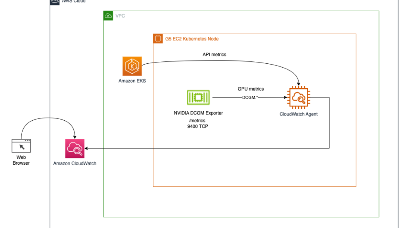
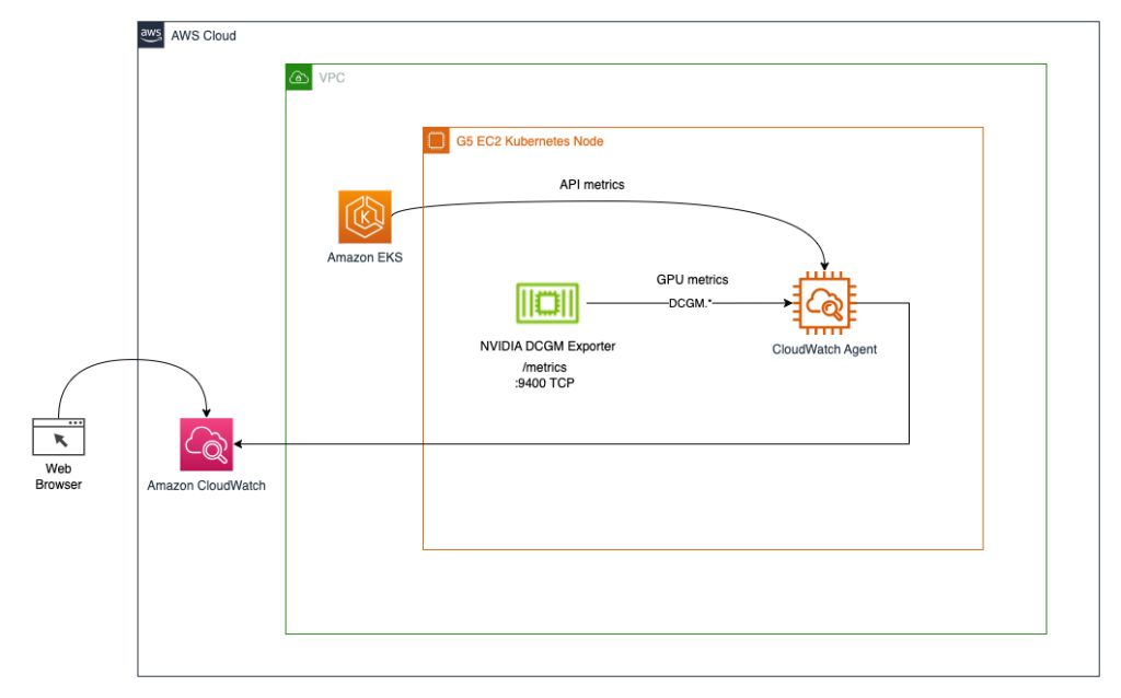
We deploy the NVIDIA GPU operator to enable use of GPU resources and the NVIDIA DCGM Exporter to enable GPU metrics collection. Then we explore two architectures. The first one connects the metrics from NVIDIA DCGM Exporter to CloudWatch via a CloudWatch agent, as shown in the following diagram.

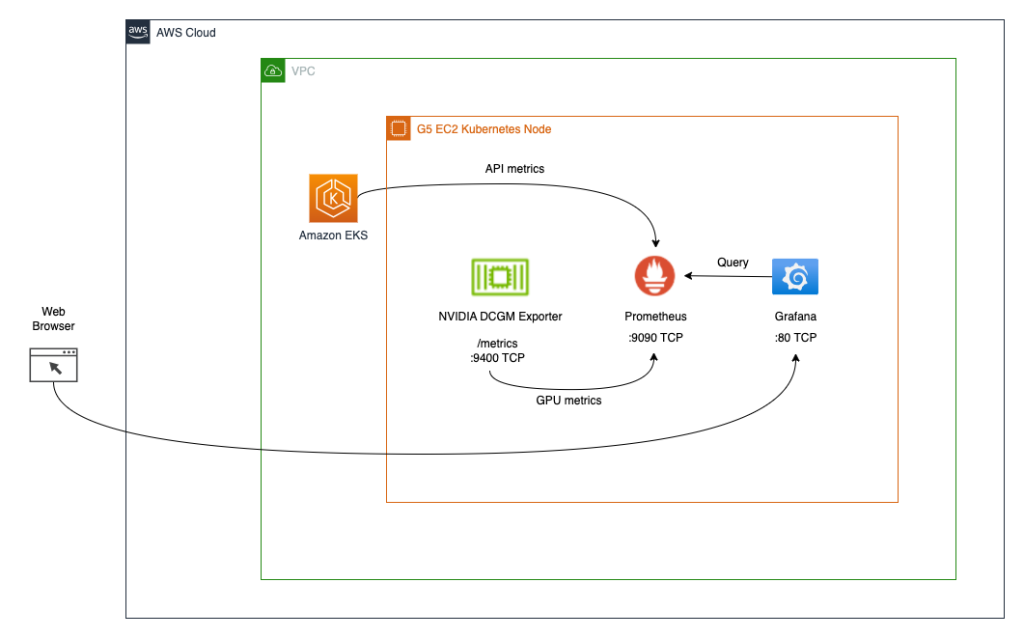
The second architecture (see the following diagram) connects the metrics from DCGM Exporter to Prometheus, then we use a Grafana dashboard to visualize those metrics.

Prerequisites

To simplify reproducing the entire stack from this post, we use a container that has all the required tooling (aws cli, eksctl, helm, etc.) already installed. In order to clone the container project from GitHub, you will need git. To build and run the container, you will need Docker. To deploy the architecture, you will need AWS credentials. To enable access to Kubernetes services using port-forwarding, you will also need kubectl.

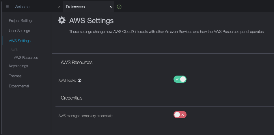
These prerequisites can be installed on your local machine, EC2 instance with NICE DCV, or AWS Cloud9. In this post, we will use a c5.2xlarge Cloud9 instance with a 40GB local storage volume. When using Cloud9, please disable AWS managed temporary credentials by visiting Cloud9->Preferences->AWS Settings as shown on the screenshot below.

Build and run the aws-do-eks container

Open a terminal shell in your preferred environment and run the following commands:

git clone https://github.com/aws-samples/aws-do-eks
cd aws-do-eks
./build.sh
./run.sh
./exec.sh

The result is as follows:

root@e5ecb162812f:/eks#

You now have a shell in a container environment that has all the tools needed to complete the tasks below. We will refer to it as “aws-do-eks shell”. You will be running the commands in the following sections in this shell, unless specifically instructed otherwise.

Create an EKS cluster with a node group

This group includes a GPU instance family of your choice; in this example, we use the g5.2xlarge instance type.

The aws-do-eks project comes with a collection of cluster configurations. You can set your desired cluster configuration with a single configuration change.

1. In the container shell, run ./env-config.sh and then set CONF=conf/eksctl/yaml/eks-gpu-g5.yaml
2. To verify the cluster configuration, run ./eks-config.sh

You should see the following cluster manifest:

apiVersion: eksctl.io/v1alpha5
kind: ClusterConfig
metadata:
  name: do-eks-yaml-g5
  version: "1.25"
  region: us-east-1
availabilityZones:
  - us-east-1a
  - us-east-1b
  - us-east-1c
  - us-east-1d
managedNodeGroups:
  - name: sys
    instanceType: m5.xlarge
    desiredCapacity: 1
    iam:
      withAddonPolicies:
        autoScaler: true
        cloudWatch: true
  - name: g5
    instanceType: g5.2xlarge
    instancePrefix: g5-2xl
    privateNetworking: true
    efaEnabled: false
    minSize: 0
    desiredCapacity: 1
    maxSize: 10
    volumeSize: 80
    iam:
      withAddonPolicies:
        cloudWatch: true
iam:
  withOIDC: true

3. To create the cluster, run the following command in the container

./eks-create.sh

The output is as follows:

root@e5ecb162812f:/eks# ./eks-create.sh 
/eks/impl/eksctl/yaml /eks

./eks-create.sh

Mon May 22 20:50:59 UTC 2023
Creating cluster using /eks/conf/eksctl/yaml/eks-gpu-g5.yaml ...

eksctl create cluster -f /eks/conf/eksctl/yaml/eks-gpu-g5.yaml

2023-05-22 20:50:59 [ℹ]  eksctl version 0.133.0
2023-05-22 20:50:59 [ℹ]  using region us-east-1
2023-05-22 20:50:59 [ℹ]  subnets for us-east-1a - public:192.168.0.0/19 private:192.168.128.0/19
2023-05-22 20:50:59 [ℹ]  subnets for us-east-1b - public:192.168.32.0/19 private:192.168.160.0/19
2023-05-22 20:50:59 [ℹ]  subnets for us-east-1c - public:192.168.64.0/19 private:192.168.192.0/19
2023-05-22 20:50:59 [ℹ]  subnets for us-east-1d - public:192.168.96.0/19 private:192.168.224.0/19
2023-05-22 20:50:59 [ℹ]  nodegroup "sys" will use "" [AmazonLinux2/1.25]
2023-05-22 20:50:59 [ℹ]  nodegroup "g5" will use "" [AmazonLinux2/1.25]
2023-05-22 20:50:59 [ℹ]  using Kubernetes version 1.25
2023-05-22 20:50:59 [ℹ]  creating EKS cluster "do-eks-yaml-g5" in "us-east-1" region with managed nodes
2023-05-22 20:50:59 [ℹ]  2 nodegroups (g5, sys) were included (based on the include/exclude rules)
2023-05-22 20:50:59 [ℹ]  will create a CloudFormation stack for cluster itself and 0 nodegroup stack(s)
2023-05-22 20:50:59 [ℹ]  will create a CloudFormation stack for cluster itself and 2 managed nodegroup stack(s)
2023-05-22 20:50:59 [ℹ]  if you encounter any issues, check CloudFormation console or try 'eksctl utils describe-stacks --region=us-east-1 --cluster=do-eks-yaml-g5'
2023-05-22 20:50:59 [ℹ]  Kubernetes API endpoint access will use default of {publicAccess=true, privateAccess=false} for cluster "do-eks-yaml-g5" in "us-east-1"
2023-05-22 20:50:59 [ℹ]  CloudWatch logging will not be enabled for cluster "do-eks-yaml-g5" in "us-east-1"
2023-05-22 20:50:59 [ℹ]  you can enable it with 'eksctl utils update-cluster-logging --enable-types={SPECIFY-YOUR-LOG-TYPES-HERE (e.g. all)} --region=us-east-1 --cluster=do-eks-yaml-g5'
2023-05-22 20:50:59 [ℹ]  
2 sequential tasks: { create cluster control plane "do-eks-yaml-g5", 
    2 sequential sub-tasks: { 
        4 sequential sub-tasks: { 
            wait for control plane to become ready,
            associate IAM OIDC provider,
            2 sequential sub-tasks: { 
                create IAM role for serviceaccount "kube-system/aws-node",
                create serviceaccount "kube-system/aws-node",
            },
            restart daemonset "kube-system/aws-node",
        },
        2 parallel sub-tasks: { 
            create managed nodegroup "sys",
            create managed nodegroup "g5",
        },
    } 
}
2023-05-22 20:50:59 [ℹ]  building cluster stack "eksctl-do-eks-yaml-g5-cluster"
2023-05-22 20:51:00 [ℹ]  deploying stack "eksctl-do-eks-yaml-g5-cluster"
2023-05-22 20:51:30 [ℹ]  waiting for CloudFormation stack "eksctl-do-eks-yaml-g5-cluster"
2023-05-22 20:52:00 [ℹ]  waiting for CloudFormation stack "eksctl-do-eks-yaml-g5-cluster"
2023-05-22 20:53:01 [ℹ]  waiting for CloudFormation stack "eksctl-do-eks-yaml-g5-cluster"
2023-05-22 20:54:01 [ℹ]  waiting for CloudFormation stack "eksctl-do-eks-yaml-g5-cluster"
2023-05-22 20:55:01 [ℹ]  waiting for CloudFormation stack "eksctl-do-eks-yaml-g5-cluster"
2023-05-22 20:56:02 [ℹ]  waiting for CloudFormation stack "eksctl-do-eks-yaml-g5-cluster"
2023-05-22 20:57:02 [ℹ]  waiting for CloudFormation stack "eksctl-do-eks-yaml-g5-cluster"
2023-05-22 20:58:02 [ℹ]  waiting for CloudFormation stack "eksctl-do-eks-yaml-g5-cluster"
2023-05-22 20:59:02 [ℹ]  waiting for CloudFormation stack "eksctl-do-eks-yaml-g5-cluster"
2023-05-22 21:00:03 [ℹ]  waiting for CloudFormation stack "eksctl-do-eks-yaml-g5-cluster"
2023-05-22 21:01:03 [ℹ]  waiting for CloudFormation stack "eksctl-do-eks-yaml-g5-cluster"
2023-05-22 21:02:03 [ℹ]  waiting for CloudFormation stack "eksctl-do-eks-yaml-g5-cluster"
2023-05-22 21:03:04 [ℹ]  waiting for CloudFormation stack "eksctl-do-eks-yaml-g5-cluster"
2023-05-22 21:05:07 [ℹ]  building iamserviceaccount stack "eksctl-do-eks-yaml-g5-addon-iamserviceaccount-kube-system-aws-node"
2023-05-22 21:05:10 [ℹ]  deploying stack "eksctl-do-eks-yaml-g5-addon-iamserviceaccount-kube-system-aws-node"
2023-05-22 21:05:10 [ℹ]  waiting for CloudFormation stack "eksctl-do-eks-yaml-g5-addon-iamserviceaccount-kube-system-aws-node"
2023-05-22 21:05:40 [ℹ]  waiting for CloudFormation stack "eksctl-do-eks-yaml-g5-addon-iamserviceaccount-kube-system-aws-node"
2023-05-22 21:05:40 [ℹ]  serviceaccount "kube-system/aws-node" already exists
2023-05-22 21:05:41 [ℹ]  updated serviceaccount "kube-system/aws-node"
2023-05-22 21:05:41 [ℹ]  daemonset "kube-system/aws-node" restarted
2023-05-22 21:05:41 [ℹ]  building managed nodegroup stack "eksctl-do-eks-yaml-g5-nodegroup-sys"
2023-05-22 21:05:41 [ℹ]  building managed nodegroup stack "eksctl-do-eks-yaml-g5-nodegroup-g5"
2023-05-22 21:05:42 [ℹ]  deploying stack "eksctl-do-eks-yaml-g5-nodegroup-sys"
2023-05-22 21:05:42 [ℹ]  waiting for CloudFormation stack "eksctl-do-eks-yaml-g5-nodegroup-sys"
2023-05-22 21:05:42 [ℹ]  deploying stack "eksctl-do-eks-yaml-g5-nodegroup-g5"
2023-05-22 21:05:42 [ℹ]  waiting for CloudFormation stack "eksctl-do-eks-yaml-g5-nodegroup-g5"
2023-05-22 21:06:12 [ℹ]  waiting for CloudFormation stack "eksctl-do-eks-yaml-g5-nodegroup-sys"
2023-05-22 21:06:12 [ℹ]  waiting for CloudFormation stack "eksctl-do-eks-yaml-g5-nodegroup-g5"
2023-05-22 21:06:55 [ℹ]  waiting for CloudFormation stack "eksctl-do-eks-yaml-g5-nodegroup-sys"
2023-05-22 21:07:11 [ℹ]  waiting for CloudFormation stack "eksctl-do-eks-yaml-g5-nodegroup-g5"
2023-05-22 21:08:29 [ℹ]  waiting for CloudFormation stack "eksctl-do-eks-yaml-g5-nodegroup-g5"
2023-05-22 21:08:45 [ℹ]  waiting for CloudFormation stack "eksctl-do-eks-yaml-g5-nodegroup-sys"
2023-05-22 21:09:52 [ℹ]  waiting for CloudFormation stack "eksctl-do-eks-yaml-g5-nodegroup-g5"
2023-05-22 21:09:53 [ℹ]  waiting for the control plane to become ready
2023-05-22 21:09:53 [✔]  saved kubeconfig as "/root/.kube/config"
2023-05-22 21:09:53 [ℹ]  1 task: { install Nvidia device plugin }
W0522 21:09:54.155837    1668 warnings.go:70] spec.template.metadata.annotations[scheduler.alpha.kubernetes.io/critical-pod]: non-functional in v1.16+; use the "priorityClassName" field instead
2023-05-22 21:09:54 [ℹ]  created "kube-system:DaemonSet.apps/nvidia-device-plugin-daemonset"
2023-05-22 21:09:54 [ℹ]  as you are using the EKS-Optimized Accelerated AMI with a GPU-enabled instance type, the Nvidia Kubernetes device plugin was automatically installed.
        to skip installing it, use --install-nvidia-plugin=false.
2023-05-22 21:09:54 [✔]  all EKS cluster resources for "do-eks-yaml-g5" have been created
2023-05-22 21:09:54 [ℹ]  nodegroup "sys" has 1 node(s)
2023-05-22 21:09:54 [ℹ]  node "ip-192-168-18-137.ec2.internal" is ready
2023-05-22 21:09:54 [ℹ]  waiting for at least 1 node(s) to become ready in "sys"
2023-05-22 21:09:54 [ℹ]  nodegroup "sys" has 1 node(s)
2023-05-22 21:09:54 [ℹ]  node "ip-192-168-18-137.ec2.internal" is ready
2023-05-22 21:09:55 [ℹ]  kubectl command should work with "/root/.kube/config", try 'kubectl get nodes'
2023-05-22 21:09:55 [✔]  EKS cluster "do-eks-yaml-g5" in "us-east-1" region is ready

Mon May 22 21:09:55 UTC 2023
Done creating cluster using /eks/conf/eksctl/yaml/eks-gpu-g5.yaml

/eks

4. To verify that your cluster is created successfully, run the following command

kubectl get nodes -L node.kubernetes.io/instance-type

The output is similar to the following:

NAME                              STATUS   ROLES    AGE   VERSION               INSTANCE_TYPE
ip-192-168-18-137.ec2.internal    Ready    <none>   47m   v1.25.9-eks-0a21954   m5.xlarge
ip-192-168-214-241.ec2.internal   Ready    <none>   46m   v1.25.9-eks-0a21954   g5.2xlarge

In this example, we have one m5.xlarge and one g5.2xlarge instance in our cluster; therefore, we see two nodes listed in the preceding output.

During the cluster creation process, the NVIDIA device plugin will get installed. You will need to remove it after cluster creation because we will use the NVIDIA GPU Operator instead.

5. Delete the plugin with the following command

kubectl -n kube-system delete daemonset nvidia-device-plugin-daemonset

We get the following output:

daemonset.apps "nvidia-device-plugin-daemonset" deleted

Install the NVIDIA Helm repo

Install the NVIDIA Helm repo with the following command:

helm repo add nvidia https://helm.ngc.nvidia.com/nvidia && helm repo update

Deploy the DCGM exporter with the NVIDIA GPU Operator

To deploy the DCGM exporter, complete the following steps:

1. Prepare the DCGM exporter GPU metrics configuration

curl https://raw.githubusercontent.com/NVIDIA/dcgm-exporter/main/etc/dcp-metrics-included.csv > dcgm-metrics.csv

You have the option to edit the dcgm-metrics.csv file. You can add or remove any metrics as needed.

2. Create the gpu-operator namespace and DCGM exporter ConfigMap

kubectl create namespace gpu-operator && /
kubectl create configmap metrics-config -n gpu-operator --from-file=dcgm-metrics.csv

The output is as follows:

namespace/gpu-operator created
configmap/metrics-config created

3. Apply the GPU operator to the EKS cluster

helm install --wait --generate-name -n gpu-operator --create-namespace nvidia/gpu-operator 
--set dcgmExporter.config.name=metrics-config 
--set dcgmExporter.env[0].name=DCGM_EXPORTER_COLLECTORS 
--set dcgmExporter.env[0].value=/etc/dcgm-exporter/dcgm-metrics.csv 
--set toolkit.enabled=false

The output is as follows:

NAME: gpu-operator-1684795140
LAST DEPLOYED: Day Month Date HH:mm:ss YYYY
NAMESPACE: gpu-operator
STATUS: deployed
REVISION: 1
TEST SUITE: None

4. Confirm that the DCGM exporter pod is running

kubectl -n gpu-operator get pods | grep dcgm

The output is as follows:

nvidia-dcgm-exporter-lkmfr       1/1     Running    0   1m

If you inspect the logs, you should see the “Starting webserver” message:

kubectl -n gpu-operator logs -f $(kubectl -n gpu-operator get pods | grep dcgm | cut -d ' ' -f 1)

The output is as follows:

Defaulted container "nvidia-dcgm-exporter" out of: nvidia-dcgm-exporter, toolkit-validation (init)
time="2023-05-22T22:40:08Z" level=info msg="Starting dcgm-exporter"
time="2023-05-22T22:40:08Z" level=info msg="DCGM successfully initialized!"
time="2023-05-22T22:40:08Z" level=info msg="Collecting DCP Metrics"
time="2023-05-22T22:40:08Z" level=info msg="No configmap data specified, falling back to metric file /etc/dcgm-exporter/dcgm-metrics.csv"
time="2023-05-22T22:40:08Z" level=info msg="Initializing system entities of type: GPU"
time="2023-05-22T22:40:09Z" level=info msg="Initializing system entities of type: NvSwitch"
time="2023-05-22T22:40:09Z" level=info msg="Not collecting switch metrics: no switches to monitor"
time="2023-05-22T22:40:09Z" level=info msg="Initializing system entities of type: NvLink"
time="2023-05-22T22:40:09Z" level=info msg="Not collecting link metrics: no switches to monitor"
time="2023-05-22T22:40:09Z" level=info msg="Kubernetes metrics collection enabled!"
time="2023-05-22T22:40:09Z" level=info msg="Pipeline starting"
time="2023-05-22T22:40:09Z" level=info msg="Starting webserver"

NVIDIA DCGM Exporter exposes a Prometheus metrics endpoint, which can be ingested by the CloudWatch agent. To see the endpoint, use the following command:

kubectl -n gpu-operator get services | grep dcgm

We get the following output:

nvidia-dcgm-exporter    ClusterIP   10.100.183.207   <none>   9400/TCP   10m

5. To generate some GPU utilization, we deploy a pod that runs the gpu-burn binary

kubectl apply -f https://raw.githubusercontent.com/aws-samples/aws-do-eks/main/Container-Root/eks/deployment/gpu-metrics/gpu-burn-deployment.yaml

The output is as follows:

deployment.apps/gpu-burn created

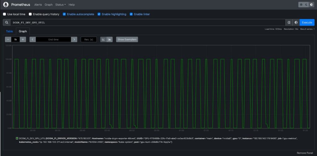
This deployment uses a single GPU to produce a continuous pattern of 100% utilization for 20 seconds followed by 0% utilization for 20 seconds.

6. To make sure the endpoint works, you can run a temporary container that uses curl to read the content of http://nvidia-dcgm-exporter:9400/metrics

kubectl -n gpu-operator run -it --rm curl --restart='Never' --image=curlimages/curl --command -- curl http://nvidia-dcgm-exporter:9400/metrics

We get the following output:

# HELP DCGM_FI_DEV_SM_CLOCK SM clock frequency (in MHz).
# TYPE DCGM_FI_DEV_SM_CLOCK gauge
DCGM_FI_DEV_SM_CLOCK{gpu="0",UUID="GPU-ff76466b-22fc-f7a9-abe2-ce3ac453b8b3",device="nvidia0",modelName="NVIDIA A10G",Hostname="nvidia-dcgm-exporter-48cwd",DCGM_FI_DRIVER_VERSION="470.182.03",container="main",namespace="kube-system",pod="gpu-burn-c68d8c774-ltg9s"} 1455
# HELP DCGM_FI_DEV_MEM_CLOCK Memory clock frequency (in MHz).
# TYPE DCGM_FI_DEV_MEM_CLOCK gauge
DCGM_FI_DEV_MEM_CLOCK{gpu="0",UUID="GPU-ff76466b-22fc-f7a9-abe2-ce3ac453b8b3",device="nvidia0",modelName="NVIDIA A10G",Hostname="nvidia-dcgm-exporter-48cwd",DCGM_FI_DRIVER_VERSION="470.182.03",container="main",namespace="kube-system",pod="gpu-burn-c68d8c774-ltg9s"} 6250
# HELP DCGM_FI_DEV_GPU_TEMP GPU temperature (in C).
# TYPE DCGM_FI_DEV_GPU_TEMP gauge
DCGM_FI_DEV_GPU_TEMP{gpu="0",UUID="GPU-ff76466b-22fc-f7a9-abe2-ce3ac453b8b3",device="nvidia0",modelName="NVIDIA A10G",Hostname="nvidia-dcgm-exporter-48cwd",DCGM_FI_DRIVER_VERSION="470.182.03",container="main",namespace="kube-system",pod="gpu-burn-c68d8c774-ltg9s"} 65
# HELP DCGM_FI_DEV_POWER_USAGE Power draw (in W).
# TYPE DCGM_FI_DEV_POWER_USAGE gauge
DCGM_FI_DEV_POWER_USAGE{gpu="0",UUID="GPU-ff76466b-22fc-f7a9-abe2-ce3ac453b8b3",device="nvidia0",modelName="NVIDIA A10G",Hostname="nvidia-dcgm-exporter-48cwd",DCGM_FI_DRIVER_VERSION="470.182.03",container="main",namespace="kube-system",pod="gpu-burn-c68d8c774-ltg9s"} 299.437000
# HELP DCGM_FI_DEV_TOTAL_ENERGY_CONSUMPTION Total energy consumption since boot (in mJ).
# TYPE DCGM_FI_DEV_TOTAL_ENERGY_CONSUMPTION counter
DCGM_FI_DEV_TOTAL_ENERGY_CONSUMPTION{gpu="0",UUID="GPU-ff76466b-22fc-f7a9-abe2-ce3ac453b8b3",device="nvidia0",modelName="NVIDIA A10G",Hostname="nvidia-dcgm-exporter-48cwd",DCGM_FI_DRIVER_VERSION="470.182.03",container="main",namespace="kube-system",pod="gpu-burn-c68d8c774-ltg9s"} 15782796862
# HELP DCGM_FI_DEV_PCIE_REPLAY_COUNTER Total number of PCIe retries.
# TYPE DCGM_FI_DEV_PCIE_REPLAY_COUNTER counter
DCGM_FI_DEV_PCIE_REPLAY_COUNTER{gpu="0",UUID="GPU-ff76466b-22fc-f7a9-abe2-ce3ac453b8b3",device="nvidia0",modelName="NVIDIA A10G",Hostname="nvidia-dcgm-exporter-48cwd",DCGM_FI_DRIVER_VERSION="470.182.03",container="main",namespace="kube-system",pod="gpu-burn-c68d8c774-ltg9s"} 0
# HELP DCGM_FI_DEV_GPU_UTIL GPU utilization (in %).
# TYPE DCGM_FI_DEV_GPU_UTIL gauge
DCGM_FI_DEV_GPU_UTIL{gpu="0",UUID="GPU-ff76466b-22fc-f7a9-abe2-ce3ac453b8b3",device="nvidia0",modelName="NVIDIA A10G",Hostname="nvidia-dcgm-exporter-48cwd",DCGM_FI_DRIVER_VERSION="470.182.03",container="main",namespace="kube-system",pod="gpu-burn-c68d8c774-ltg9s"} 100
# HELP DCGM_FI_DEV_MEM_COPY_UTIL Memory utilization (in %).
# TYPE DCGM_FI_DEV_MEM_COPY_UTIL gauge
DCGM_FI_DEV_MEM_COPY_UTIL{gpu="0",UUID="GPU-ff76466b-22fc-f7a9-abe2-ce3ac453b8b3",device="nvidia0",modelName="NVIDIA A10G",Hostname="nvidia-dcgm-exporter-48cwd",DCGM_FI_DRIVER_VERSION="470.182.03",container="main",namespace="kube-system",pod="gpu-burn-c68d8c774-ltg9s"} 38
# HELP DCGM_FI_DEV_ENC_UTIL Encoder utilization (in %).
# TYPE DCGM_FI_DEV_ENC_UTIL gauge
DCGM_FI_DEV_ENC_UTIL{gpu="0",UUID="GPU-ff76466b-22fc-f7a9-abe2-ce3ac453b8b3",device="nvidia0",modelName="NVIDIA A10G",Hostname="nvidia-dcgm-exporter-48cwd",DCGM_FI_DRIVER_VERSION="470.182.03",container="main",namespace="kube-system",pod="gpu-burn-c68d8c774-ltg9s"} 0
# HELP DCGM_FI_DEV_DEC_UTIL Decoder utilization (in %).
# TYPE DCGM_FI_DEV_DEC_UTIL gauge
DCGM_FI_DEV_DEC_UTIL{gpu="0",UUID="GPU-ff76466b-22fc-f7a9-abe2-ce3ac453b8b3",device="nvidia0",modelName="NVIDIA A10G",Hostname="nvidia-dcgm-exporter-48cwd",DCGM_FI_DRIVER_VERSION="470.182.03",container="main",namespace="kube-system",pod="gpu-burn-c68d8c774-ltg9s"} 0
# HELP DCGM_FI_DEV_XID_ERRORS Value of the last XID error encountered.
# TYPE DCGM_FI_DEV_XID_ERRORS gauge
DCGM_FI_DEV_XID_ERRORS{gpu="0",UUID="GPU-ff76466b-22fc-f7a9-abe2-ce3ac453b8b3",device="nvidia0",modelName="NVIDIA A10G",Hostname="nvidia-dcgm-exporter-48cwd",DCGM_FI_DRIVER_VERSION="470.182.03",container="main",namespace="kube-system",pod="gpu-burn-c68d8c774-ltg9s"} 0
# HELP DCGM_FI_DEV_FB_FREE Framebuffer memory free (in MiB).
# TYPE DCGM_FI_DEV_FB_FREE gauge
DCGM_FI_DEV_FB_FREE{gpu="0",UUID="GPU-ff76466b-22fc-f7a9-abe2-ce3ac453b8b3",device="nvidia0",modelName="NVIDIA A10G",Hostname="nvidia-dcgm-exporter-48cwd",DCGM_FI_DRIVER_VERSION="470.182.03",container="main",namespace="kube-system",pod="gpu-burn-c68d8c774-ltg9s"} 2230
# HELP DCGM_FI_DEV_FB_USED Framebuffer memory used (in MiB).
# TYPE DCGM_FI_DEV_FB_USED gauge
DCGM_FI_DEV_FB_USED{gpu="0",UUID="GPU-ff76466b-22fc-f7a9-abe2-ce3ac453b8b3",device="nvidia0",modelName="NVIDIA A10G",Hostname="nvidia-dcgm-exporter-48cwd",DCGM_FI_DRIVER_VERSION="470.182.03",container="main",namespace="kube-system",pod="gpu-burn-c68d8c774-ltg9s"} 20501
# HELP DCGM_FI_DEV_NVLINK_BANDWIDTH_TOTAL Total number of NVLink bandwidth counters for all lanes.
# TYPE DCGM_FI_DEV_NVLINK_BANDWIDTH_TOTAL counter
DCGM_FI_DEV_NVLINK_BANDWIDTH_TOTAL{gpu="0",UUID="GPU-ff76466b-22fc-f7a9-abe2-ce3ac453b8b3",device="nvidia0",modelName="NVIDIA A10G",Hostname="nvidia-dcgm-exporter-48cwd",DCGM_FI_DRIVER_VERSION="470.182.03",container="main",namespace="kube-system",pod="gpu-burn-c68d8c774-ltg9s"} 0
# HELP DCGM_FI_DEV_VGPU_LICENSE_STATUS vGPU License status
# TYPE DCGM_FI_DEV_VGPU_LICENSE_STATUS gauge
DCGM_FI_DEV_VGPU_LICENSE_STATUS{gpu="0",UUID="GPU-ff76466b-22fc-f7a9-abe2-ce3ac453b8b3",device="nvidia0",modelName="NVIDIA A10G",Hostname="nvidia-dcgm-exporter-48cwd",DCGM_FI_DRIVER_VERSION="470.182.03",container="main",namespace="kube-system",pod="gpu-burn-c68d8c774-ltg9s"} 0
# HELP DCGM_FI_DEV_UNCORRECTABLE_REMAPPED_ROWS Number of remapped rows for uncorrectable errors
# TYPE DCGM_FI_DEV_UNCORRECTABLE_REMAPPED_ROWS counter
DCGM_FI_DEV_UNCORRECTABLE_REMAPPED_ROWS{gpu="0",UUID="GPU-ff76466b-22fc-f7a9-abe2-ce3ac453b8b3",device="nvidia0",modelName="NVIDIA A10G",Hostname="nvidia-dcgm-exporter-48cwd",DCGM_FI_DRIVER_VERSION="470.182.03",container="main",namespace="kube-system",pod="gpu-burn-c68d8c774-ltg9s"} 0
# HELP DCGM_FI_DEV_CORRECTABLE_REMAPPED_ROWS Number of remapped rows for correctable errors
# TYPE DCGM_FI_DEV_CORRECTABLE_REMAPPED_ROWS counter
DCGM_FI_DEV_CORRECTABLE_REMAPPED_ROWS{gpu="0",UUID="GPU-ff76466b-22fc-f7a9-abe2-ce3ac453b8b3",device="nvidia0",modelName="NVIDIA A10G",Hostname="nvidia-dcgm-exporter-48cwd",DCGM_FI_DRIVER_VERSION="470.182.03",container="main",namespace="kube-system",pod="gpu-burn-c68d8c774-ltg9s"} 0
# HELP DCGM_FI_DEV_ROW_REMAP_FAILURE Whether remapping of rows has failed
# TYPE DCGM_FI_DEV_ROW_REMAP_FAILURE gauge
DCGM_FI_DEV_ROW_REMAP_FAILURE{gpu="0",UUID="GPU-ff76466b-22fc-f7a9-abe2-ce3ac453b8b3",device="nvidia0",modelName="NVIDIA A10G",Hostname="nvidia-dcgm-exporter-48cwd",DCGM_FI_DRIVER_VERSION="470.182.03",container="main",namespace="kube-system",pod="gpu-burn-c68d8c774-ltg9s"} 0
# HELP DCGM_FI_PROF_GR_ENGINE_ACTIVE Ratio of time the graphics engine is active (in %).
# TYPE DCGM_FI_PROF_GR_ENGINE_ACTIVE gauge
DCGM_FI_PROF_GR_ENGINE_ACTIVE{gpu="0",UUID="GPU-ff76466b-22fc-f7a9-abe2-ce3ac453b8b3",device="nvidia0",modelName="NVIDIA A10G",Hostname="nvidia-dcgm-exporter-48cwd",DCGM_FI_DRIVER_VERSION="470.182.03",container="main",namespace="kube-system",pod="gpu-burn-c68d8c774-ltg9s"} 0.808369
# HELP DCGM_FI_PROF_PIPE_TENSOR_ACTIVE Ratio of cycles the tensor (HMMA) pipe is active (in %).
# TYPE DCGM_FI_PROF_PIPE_TENSOR_ACTIVE gauge
DCGM_FI_PROF_PIPE_TENSOR_ACTIVE{gpu="0",UUID="GPU-ff76466b-22fc-f7a9-abe2-ce3ac453b8b3",device="nvidia0",modelName="NVIDIA A10G",Hostname="nvidia-dcgm-exporter-48cwd",DCGM_FI_DRIVER_VERSION="470.182.03",container="main",namespace="kube-system",pod="gpu-burn-c68d8c774-ltg9s"} 0.000000
# HELP DCGM_FI_PROF_DRAM_ACTIVE Ratio of cycles the device memory interface is active sending or receiving data (in %).
# TYPE DCGM_FI_PROF_DRAM_ACTIVE gauge
DCGM_FI_PROF_DRAM_ACTIVE{gpu="0",UUID="GPU-ff76466b-22fc-f7a9-abe2-ce3ac453b8b3",device="nvidia0",modelName="NVIDIA A10G",Hostname="nvidia-dcgm-exporter-48cwd",DCGM_FI_DRIVER_VERSION="470.182.03",container="main",namespace="kube-system",pod="gpu-burn-c68d8c774-ltg9s"} 0.315787
# HELP DCGM_FI_PROF_PCIE_TX_BYTES The rate of data transmitted over the PCIe bus - including both protocol headers and data payloads - in bytes per second.
# TYPE DCGM_FI_PROF_PCIE_TX_BYTES gauge
DCGM_FI_PROF_PCIE_TX_BYTES{gpu="0",UUID="GPU-ff76466b-22fc-f7a9-abe2-ce3ac453b8b3",device="nvidia0",modelName="NVIDIA A10G",Hostname="nvidia-dcgm-exporter-48cwd",DCGM_FI_DRIVER_VERSION="470.182.03",container="main",namespace="kube-system",pod="gpu-burn-c68d8c774-ltg9s"} 3985328
# HELP DCGM_FI_PROF_PCIE_RX_BYTES The rate of data received over the PCIe bus - including both protocol headers and data payloads - in bytes per second.
# TYPE DCGM_FI_PROF_PCIE_RX_BYTES gauge
DCGM_FI_PROF_PCIE_RX_BYTES{gpu="0",UUID="GPU-ff76466b-22fc-f7a9-abe2-ce3ac453b8b3",device="nvidia0",modelName="NVIDIA A10G",Hostname="nvidia-dcgm-exporter-48cwd",DCGM_FI_DRIVER_VERSION="470.182.03",container="main",namespace="kube-system",pod="gpu-burn-c68d8c774-ltg9s"} 21715174
pod "curl" deleted

Configure and deploy the CloudWatch agent

To configure and deploy the CloudWatch agent, complete the following steps:

1. Download the YAML file and edit it

curl -O https://raw.githubusercontent.com/aws-samples/amazon-cloudwatch-container-insights/k8s/1.3.15/k8s-deployment-manifest-templates/deployment-mode/service/cwagent-prometheus/prometheus-eks.yaml

The file contains a cwagent configmap and a prometheus configmap. For this post, we edit both.

2. Edit the prometheus-eks.yaml file

Open the prometheus-eks.yaml file in your favorite editor and replace the cwagentconfig.json section with the following content:

apiVersion: v1
data:
  # cwagent json config
  cwagentconfig.json: |
    {
      "logs": {
        "metrics_collected": {
          "prometheus": {
            "prometheus_config_path": "/etc/prometheusconfig/prometheus.yaml",
            "emf_processor": {
              "metric_declaration": [
                {
                  "source_labels": ["Service"],
                  "label_matcher": ".*dcgm.*",
                  "dimensions": [["Service","Namespace","ClusterName","job","pod"]],
                  "metric_selectors": [
                    "^DCGM_FI_DEV_GPU_UTIL$",
                    "^DCGM_FI_DEV_DEC_UTIL$",
                    "^DCGM_FI_DEV_ENC_UTIL$",
                    "^DCGM_FI_DEV_MEM_CLOCK$",
                    "^DCGM_FI_DEV_MEM_COPY_UTIL$",
                    "^DCGM_FI_DEV_POWER_USAGE$",
                    "^DCGM_FI_DEV_ROW_REMAP_FAILURE$",
                    "^DCGM_FI_DEV_SM_CLOCK$",
                    "^DCGM_FI_DEV_XID_ERRORS$",
                    "^DCGM_FI_PROF_DRAM_ACTIVE$",
                    "^DCGM_FI_PROF_GR_ENGINE_ACTIVE$",
                    "^DCGM_FI_PROF_PCIE_RX_BYTES$",
                    "^DCGM_FI_PROF_PCIE_TX_BYTES$",
                    "^DCGM_FI_PROF_PIPE_TENSOR_ACTIVE$"
                  ]
                }
              ]
            }
          }
        },
        "force_flush_interval": 5
      }
    }

3. In the prometheus config section, append the following job definition for the DCGM exporter

- job_name: 'kubernetes-pod-dcgm-exporter'
      sample_limit: 10000
      metrics_path: /api/v1/metrics/prometheus
      kubernetes_sd_configs:
      - role: pod
      relabel_configs:
      - source_labels: [__meta_kubernetes_pod_container_name]
        action: keep
        regex: '^DCGM.*$'
      - source_labels: [__address__]
        action: replace
        regex: ([^:]+)(?::d+)?
        replacement: ${1}:9400
        target_label: __address__
      - action: labelmap
        regex: __meta_kubernetes_pod_label_(.+)
      - action: replace
        source_labels:
        - __meta_kubernetes_namespace
        target_label: Namespace
      - source_labels: [__meta_kubernetes_pod]
        action: replace
        target_label: pod
      - action: replace
        source_labels:
        - __meta_kubernetes_pod_container_name
        target_label: container_name
      - action: replace
        source_labels:
        - __meta_kubernetes_pod_controller_name
        target_label: pod_controller_name
      - action: replace
        source_labels:
        - __meta_kubernetes_pod_controller_kind
        target_label: pod_controller_kind
      - action: replace
        source_labels:
        - __meta_kubernetes_pod_phase
        target_label: pod_phase
      - action: replace
        source_labels:
        - __meta_kubernetes_pod_node_name
        target_label: NodeName

4. Save the file and apply the cwagent-dcgm configuration to your cluster

kubectl apply -f ./prometheus-eks.yaml

We get the following output:

namespace/amazon-cloudwatch created
configmap/prometheus-cwagentconfig created
configmap/prometheus-config created
serviceaccount/cwagent-prometheus created
clusterrole.rbac.authorization.k8s.io/cwagent-prometheus-role created
clusterrolebinding.rbac.authorization.k8s.io/cwagent-prometheus-role-binding created
deployment.apps/cwagent-prometheus created

5. Confirm that the CloudWatch agent pod is running

kubectl -n amazon-cloudwatch get pods

We get the following output:

NAME                                  READY   STATUS    RESTARTS   AGE
cwagent-prometheus-7dfd69cc46-s4cx7   1/1     Running   0          15m

Visualize metrics on the CloudWatch console

To visualize the metrics in CloudWatch, complete the following steps:

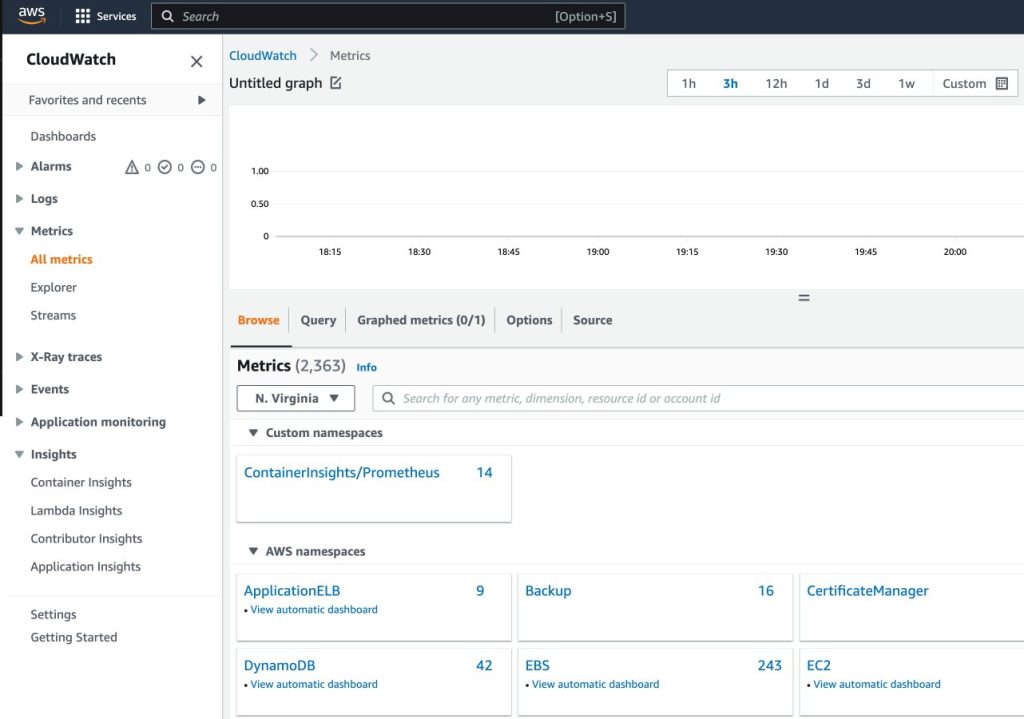
1. On the CloudWatch console, under Metrics in the navigation pane, choose All metrics
2. In the Custom namespaces section, choose the new entry for ContainerInsights/Prometheus

For more information about the ContainerInsights/Prometheus namespace, refer to Scraping additional Prometheus sources and importing those metrics.

3. Drill down to the metric names and choose DCGM_FI_DEV_GPU_UTIL
4. On the Graphed metrics tab, set Period to 5 seconds

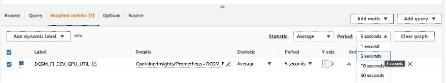
5. Set the refresh interval to 10 seconds

You will see the metrics collected from DCGM exporter that visualize the gpu-burn pattern on and off each 20 seconds.

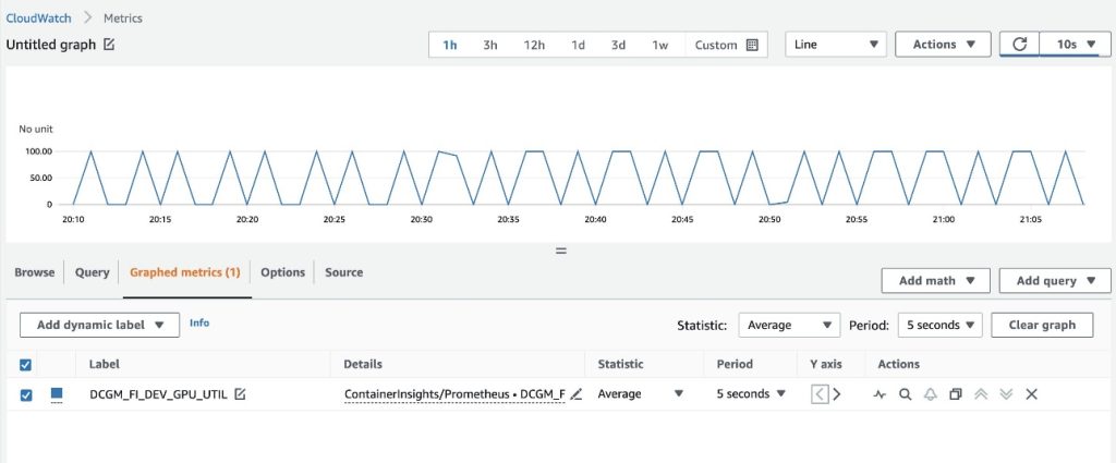
On the Browse tab, you can see the data, including the pod name for each metric.

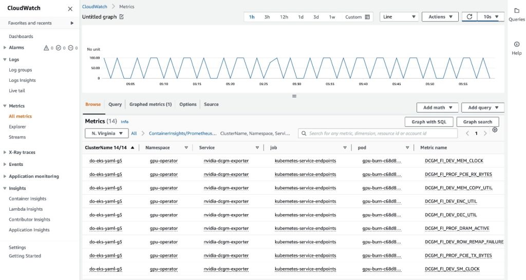
The EKS API metadata has been combined with the DCGM metrics data, resulting in the provided pod-based GPU metrics.

This concludes the first approach of exporting DCGM metrics to CloudWatch via the CloudWatch agent.

In the next section, we configure the second architecture, which exports the DCGM metrics to Prometheus, and we visualize them with Grafana.

Use Prometheus and Grafana to visualize GPU metrics from DCGM

Complete the following steps:

1. Add the Prometheus community helm chart

helm repo add prometheus-community https://prometheus-community.github.io/helm-charts

This chart deploys both Prometheus and Grafana. We need to make some edits to the chart before running the install command.

2. Save the chart configuration values to a file in /tmp

helm inspect values prometheus-community/kube-prometheus-stack > /tmp/kube-prometheus-stack.values

3. Edit the char configuration file

Edit the saved file (/tmp/kube-prometheus-stack.values) and set the following option by looking for the setting name and setting the value:

prometheus.prometheusSpec.serviceMonitorSelectorNilUsesHelmValues=false

4. Add the following ConfigMap to the additionalScrapeConfigs section

additionalScrapeConfigs:
- job_name: gpu-metrics
  scrape_interval: 1s
  metrics_path: /metrics
  scheme: http
  kubernetes_sd_configs:
  - role: endpoints
    namespaces:
      names:
      - gpu-operator
  relabel_configs:
  - source_labels: [__meta_kubernetes_pod_node_name]
    action: replace
    target_label: kubernetes_node

5. Deploy the Prometheus stack with the updated values

helm install prometheus-community/kube-prometheus-stack 
--create-namespace --namespace prometheus 
--generate-name 
--values /tmp/kube-prometheus-stack.values

We get the following output:

NAME: kube-prometheus-stack-1684965548
LAST DEPLOYED: Wed May 24 21:59:14 2023
NAMESPACE: prometheus
STATUS: deployed
REVISION: 1
NOTES:
kube-prometheus-stack has been installed. Check its status by running:
  kubectl --namespace prometheus get pods -l "release=kube-prometheus-stack-1684965548"

Visit https://github.com/prometheus-operator/kube-prometheus
 for instructions on how to create & configure Alertmanager 
and Prometheus instances using the Operator.

6. Confirm that the Prometheus pods are running

kubectl get pods -n prometheus

We get the following output:

NAME                                                              READY   STATUS    RESTARTS   AGE
alertmanager-kube-prometheus-stack-1684-alertmanager-0            2/2     Running   0          6m55s
kube-prometheus-stack-1684-operator-6c87649878-j7v55              1/1     Running   0          6m58s
kube-prometheus-stack-1684965548-grafana-dcd7b4c96-bzm8p          3/3     Running   0          6m58s
kube-prometheus-stack-1684965548-kube-state-metrics-7d856dptlj5   1/1     Running   0          6m58s
kube-prometheus-stack-1684965548-prometheus-node-exporter-2fbl5   1/1     Running   0          6m58s
kube-prometheus-stack-1684965548-prometheus-node-exporter-m7zmv   1/1     Running   0          6m58s
prometheus-kube-prometheus-stack-1684-prometheus-0                2/2     Running   0          6m55s

Prometheus and Grafana pods are in the Running state.

Next, we validate that DCGM metrics are flowing into Prometheus.

7. Port-forward the Prometheus UI

There are different ways to expose the Prometheus UI running in EKS to requests originating outside of the cluster. We will use kubectl port-forwarding. So far, we have been executing commands inside the aws-do-eks container. To access the Prometheus service running in the cluster, we will create a tunnel from the host. Here the aws-do-eks container is running by executing the following command outside of the container, in a new terminal shell on the host. We will refer to this as “host shell”.

kubectl -n prometheus port-forward svc/$(kubectl -n prometheus get svc | grep prometheus | grep -v alertmanager | grep -v operator | grep -v grafana | grep -v metrics | grep -v exporter | grep -v operated | cut -d ' ' -f 1) 8080:9090 &

8. Open the Prometheus UI
   • If you are using Cloud9, please navigate to Preview->Preview Running Application to open the Prometheus UI in a tab inside the Cloud9 IDE, then click the icon in the upper-right corner of the tab to pop out in a new window.
   • If you are on your local host or connected to an EC2 instance via remote desktop open a browser and visit the URL http://localhost:8080.

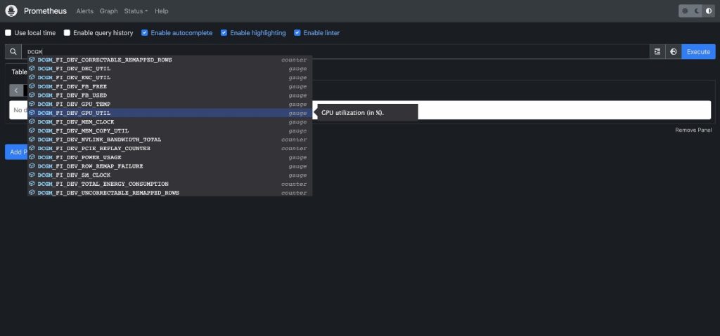
9. Enter DCGM to see the DCGM metrics that are flowing into Prometheus
10. Select DCGM_FI_DEV_GPU_UTIL, choose Execute, and then navigate to the Graph tab to see the expected GPU utilization pattern

11. Stop the Prometheus port-forwarding process

Run the following command line in your host shell:

kill -9 $(ps -aef | grep port-forward | grep -v grep | grep prometheus | awk '{print $2}')

Now we can visualize the DCGM metrics via Grafana Dashboard.

12. Retrieve the password to log in to the Grafana UI

kubectl -n prometheus get secret $(kubectl -n prometheus get secrets | grep grafana | cut -d ' ' -f 1) -o jsonpath="{.data.admin-password}" | base64 --decode ; echo

13. Port-forward the Grafana service

Run the following command line in your host shell:

kubectl port-forward -n prometheus svc/$(kubectl -n prometheus get svc | grep grafana | cut -d ' ' -f 1) 8080:80 &

14. Log in to the Grafana UI

Access the Grafana UI login screen the same way as you accessed the Prometheus UI earlier. If using Cloud9, select Preview->Preview Running Application, then pop out in a new window. If using your local host or an EC2 instance with remote desktop visit URL http://localhost:8080. Login with the user name admin and the password you retrieved earlier.

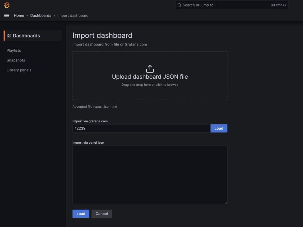
15. In the navigation pane, choose Dashboards

16. Choose New and Import

We are going to import the default DCGM Grafana dashboard described in NVIDIA DCGM Exporter Dashboard.

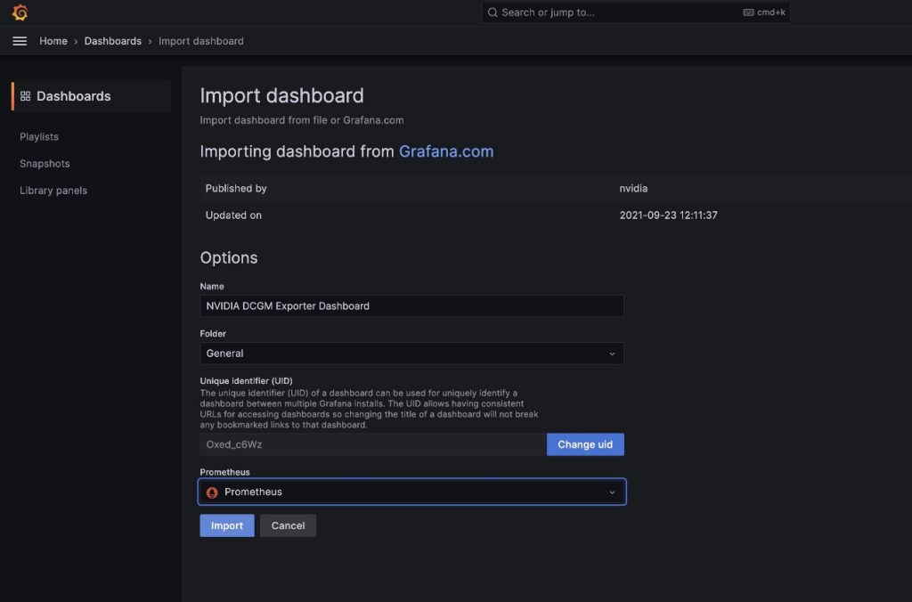
17. In the field import via grafana.com, enter 12239 and choose Load
18. Choose Prometheus as the data source
19. Choose Import

You will see a dashboard similar to the one in the following screenshot.

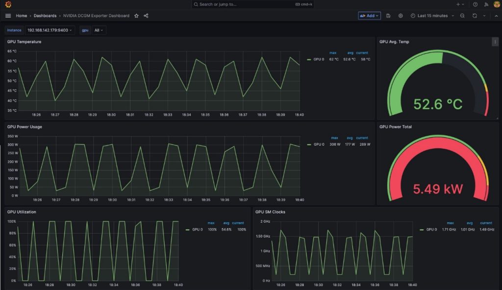
To demonstrate that these metrics are pod-based, we are going to modify the GPU Utilization pane in this dashboard.

20. Choose the pane and the options menu (three dots)
21. Expand the Options section and edit the Legend field
22. Replace the value there with Pod {{pod}}, then choose Save

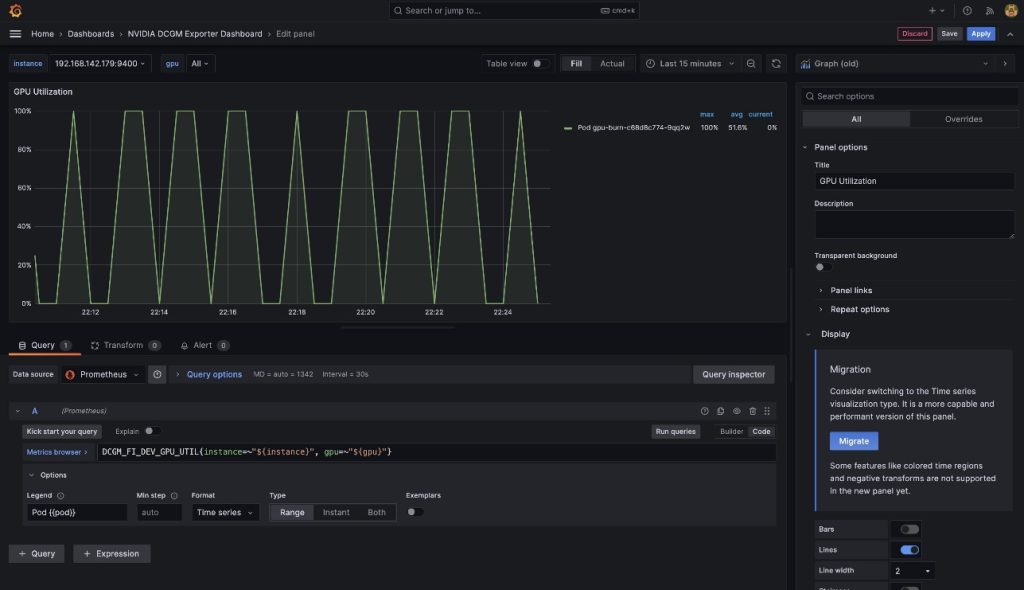
The legend now shows the gpu-burn pod name associated with the displayed GPU utilization.

23. Stop port-forwarding the Grafana UI service

Run the following in your host shell:

kill -9 $(ps -aef | grep port-forward | grep -v grep | grep prometheus | awk '{print $2}')

In this post, we demonstrated using open-source Prometheus and Grafana deployed to the EKS cluster. If desired, this deployment can be substituted with Amazon Managed Service for Prometheus and Amazon Managed Grafana.

Clean up

To clean up the resources you created, run the following script from the aws-do-eks container shell:

./eks-delete.sh

Conclusion

In this post, we utilized NVIDIA DCGM Exporter to collect GPU metrics and visualize them with either CloudWatch or Prometheus and Grafana. We invite you to use the architectures demonstrated here to enable GPU utilization monitoring with NVIDIA DCGM in your own AWS environment.

Additional resources

• Amazon EC2 GPU instances
• NVIDIA DCGM: Manage and Monitor GPUs in Cluster Environments
• kube-prometheus-stack GitHub repo

About the authors

Amr Ragab is a former Principal Solutions Architect, EC2 Accelerated Computing at AWS. He is devoted to helping customers run computational workloads at scale. In his spare time, he likes traveling and finding new ways to integrate technology into daily life.

Alex Iankoulski is a Principal Solutions Architect, Self-managed Machine Learning at AWS. He’s a full-stack software and infrastructure engineer who likes to do deep, hands-on work. In his role, he focuses on helping customers with containerization and orchestration of ML and AI workloads on container-powered AWS services. He is also the author of the open-source do framework and a Docker captain who loves applying container technologies to accelerate the pace of innovation while solving the world’s biggest challenges. During the past 10 years, Alex has worked on democratizing AI and ML, combating climate change, and making travel safer, healthcare better, and energy smarter.

Keita Watanabe is a Senior Solutions Architect of Frameworks ML Solutions at Amazon Web Services where he helps develop the industry’s best cloud based Self-managed Machine Learning solutions. His background is in Machine Learning research and development. Prior to joining AWS, Keita was working in the e-commerce industry. Keita holds a Ph.D. in Science from the University of Tokyo.

Read More

Amazon SageMaker Pipelines is a fully managed AWS service for building and orchestrating machine learning (ML) workflows. SageMaker Pipelines offers ML application developers the ability to orchestrate different steps of the ML workflow, including data loading, data transformation, training, tuning, and deployment. You can use SageMaker Pipelines to orchestrate ML jobs in SageMaker, and its integration with the larger AWS ecosystem also allows you to use resources like AWS Lambda functions, Amazon EMR jobs, and more. This enables you to build a customized and reproducible pipeline for specific requirements in your ML workflows.

In this post, we provide some best practices to maximize the value of SageMaker Pipelines and make the development experience seamless. We also discuss some common design scenarios and patterns when building SageMaker Pipelines and provide examples for addressing them.

Best practices for SageMaker Pipelines

In this section, we discuss some best practices that can be followed while designing workflows using SageMaker Pipelines. Adopting them can improve the development process and streamline the operational management of SageMaker Pipelines.

Use Pipeline Session for lazy loading of the pipeline

Pipeline Session enables lazy initialization of pipeline resources (the jobs are not started until pipeline runtime). The PipelineSession context inherits the SageMaker Session and implements convenient methods for interacting with other SageMaker entities and resources, such as training jobs, endpoints, input datasets in Amazon Simple Storage Service (Amazon S3), and so on. When defining SageMaker Pipelines, you should use PipelineSession over the regular SageMaker Session:

from sagemaker.workflow.pipeline_context import PipelineSession
from sagemaker.sklearn.processing import SKLearnProcessor
role = sagemaker.get_execution_role()
pipeline_session = PipelineSession()
sklearn_processor = SKLearnProcessor(
    framework_version=’0.20.0’,
    instance_type=’ml.m5.xlarge’,
    instance_count=1,
    base_job_name="sklearn-abalone-process",
    role=role,
    sagemaker_session=pipeline_session,
)

Run pipelines in local mode for cost-effective and quick iterations during development

You can run a pipeline in local mode using the LocalPipelineSession context. In this mode, the pipeline and jobs are run locally using resources on the local machine, instead of SageMaker managed resources. Local mode provides a cost-effective way to iterate on the pipeline code with a smaller subset of data. After the pipeline is tested locally, it can be scaled to run using the PipelineSession context.

from sagemaker.sklearn.processing import SKLearnProcessor
from sagemaker.workflow.pipeline_context import LocalPipelineSession
local_pipeline_session = LocalPipelineSession()
role = sagemaker.get_execution_role()
sklearn_processor = SKLearnProcessor(
    framework_version=’0.20.0’,
    instance_type=’ml.m5.xlarge,
    instance_count=1,
    base_job_name="sklearn-abalone-process",
    role=role,
    sagemaker_session=local_pipeline_session,
)

Manage a SageMaker pipeline through versioning

Versioning of artifacts and pipeline definitions is a common requirement in the development lifecycle. You can create multiple versions of the pipeline by naming pipeline objects with a unique prefix or suffix, the most common being a timestamp, as shown in the following code:

from sagemaker.workflow.pipeline_context import PipelineSession
import time

current_time = time.strftime("%Y-%m-%d-%H-%M-%S", time.gmtime())
pipeline_name = "pipeline_" + current_time
pipeline_session = PipelineSession()
pipeline = Pipeline(
    name=pipeline_name,
    steps=[step_process, step_train, step_eval, step_cond],
    sagemaker_session=pipeline_session,
)

Organize and track SageMaker pipeline runs by integrating with SageMaker Experiments

SageMaker Pipelines can be easily integrated with SageMaker Experiments for organizing and tracking pipeline runs. This is achieved by specifying PipelineExperimentConfig at the time of creating a pipeline object. With this configuration object, you can specify an experiment name and a trial name. The run details of a SageMaker pipeline get organized under the specified experiment and trial. If you don’t explicitly specify an experiment name, a pipeline name is used for the experiment name. Similarly, if you don’t explicitly specify a trial name, a pipeline run ID is used for the trial or run group name. See the following code:

Pipeline(
    name="MyPipeline",
    parameters=[...],
    pipeline_experiment_config=PipelineExperimentConfig(
        experiment_name = ExecutionVariables.PIPELINE_NAME,
        trial_name = ExecutionVariables.PIPELINE_EXECUTION_ID
        ),
    steps=[...]
)

Securely run SageMaker pipelines within a private VPC

To secure the ML workloads, it’s a best practice to deploy the jobs orchestrated by SageMaker Pipelines in a secure network configuration within a private VPC, private subnets, and security groups. To ensure and enforce the usage of this secure environment, you can implement the following AWS Identity and Access Management (IAM) policy for the SageMaker execution role (this is the role assumed by the pipeline during its run). You can also add the policy to run the jobs orchestrated by SageMaker Pipelines in network isolation mode.

# IAM Policy to enforce execution within a private VPC

{

    "Action": [

        "sagemaker:CreateProcessingJob",
        "sagemaker:CreateTrainingJob",
        "sagemaker:CreateModel"
    ],

    "Resource": "*",
    "Effect": "Deny",
    "Condition": {
        "Null": {
            "sagemaker:VpcSubnets": "true"
        }
    }
}

# IAM Policy to enforce execution in network isolation mode
{

    "Version": "2012-10-17",
    "Statement": [
        {
            "Effect": "Deny",
            "Action": [
                "sagemaker:Create*"
            ],
            "Resource": "*",
            "Condition": {
                "StringNotEqualsIfExists": {
                    "sagemaker:NetworkIsolation": "true"
                }
            }
        }
    ]
}

For an example of pipeline implementation with these security controls in place, refer to Orchestrating Jobs, Model Registration, and Continuous Deployment with Amazon SageMaker in a secure environment.

Monitor the cost of pipeline runs using tags

Using SageMaker pipelines by itself is free; you pay for the compute and storage resources you spin up as part of the individual pipeline steps like processing, training, and batch inference. To aggregate the costs per pipeline run, you can include tags in every pipeline step that creates a resource. These tags can then be referenced in the cost explorer to filter and aggregate total pipeline run cost, as shown in the following example:

sklearn_processor = SKLearnProcessor(
    framework_version=’0.20.0’,
    instance_type=’ml.m5.xlarge,
    instance_count=1,
    base_job_name="sklearn-abalone-process",
    role=role,
    tags=[{'Key':'pipeline-cost-tag', 'Value':'<<tag_parameter>>'}]
)

step_process = ProcessingStep(
    name="AbaloneProcess",
    processor=sklearn_processor,
    ...
)

From the cost explorer, you can now get the cost filtered by the tag:

response = client.get_cost_and_usage(
    TimePeriod={
        'Start': '2023-07-01',
        'End': '2023-07-15'
        },
    Metrics=['BLENDED_COST','USAGE_QUANTITY','UNBLENDED_COST'],
    Granularity='MONTHLY',
    Filter={
        'Dimensions': {
            'Key':'USAGE_TYPE',
            'Values': [
                ‘SageMaker:Pipeline’
            ]
        },
        'Tags': {
            'Key': 'keyName',
            'Values': [
                'keyValue',
                ]
        }
    }
)

Design patterns for some common scenarios

In this section, we discuss design patterns for some common use cases with SageMaker Pipelines.

Run a lightweight Python function using a Lambda step

Python functions are omnipresent in ML workflows; they are used in preprocessing, postprocessing, evaluation, and more. Lambda is a serverless compute service that lets you run code without provisioning or managing servers. With Lambda, you can run code in your preferred language that includes Python. You can use this to run custom Python code as part of your pipeline. A Lambda step enables you to run Lambda functions as part of your SageMaker pipeline. Start with the following code:

%%writefile lambdafunc.py

import json

def lambda_handler(event, context):
    str1 = event["str1"]
    str2 = event["str2"]
    str3 = str1 + str2
    return {
        "str3": str3
    }

Create the Lambda function using the SageMaker Python SDK’s Lambda helper:

from sagemaker.lambda_helper import Lambda

def create_lambda(function_name, script, handler):
    response = Lambda(
        function_name=function_name,
        execution_role_arn=role,
        script= script,
        handler=handler,
        timeout=600,
        memory_size=10240,
    ).upsert()

    function_arn = response['FunctionArn']
    return function_arn

fn_arn = create_Lambda("func", "lambdafunc.py", handler = "lambdafunc.lambda_handler")

Call the Lambda step:

from sagemaker.lambda_helper import Lambda
from sagemaker.workflow.lambda_step import (
    LambdaStep,
    LambdaOutput,
    LambdaOutputTypeEnum
)

str3 = LambdaOutput(output_name="str3", output_type=LambdaOutputTypeEnum.String)

# Lambda Step
step_lambda1 = LambdaStep(
    name="LambdaStep1",
    lambda_func=Lambda(
        function_arn=fn_arn
    ),
    inputs={
        "str1": "Hello",
        "str2": " World"
    },
    outputs=[str3],
)

Pass data between steps

Input data for a pipeline step is either an accessible data location or data generated by one of the previous steps in the pipeline. You can provide this information as a ProcessingInput parameter. Let’s look at a few scenarios of how you can use ProcessingInput.

Scenario 1: Pass the output (primitive data types) of a Lambda step to a processing step

Primitive data types refer to scalar data types like string, integer, Boolean, and float.

The following code snippet defines a Lambda function that returns a dictionary of variables with primitive data types. Your Lambda function code will return a JSON of key-value pairs when invoked from the Lambda step within the SageMaker pipeline.

def handler(event, context):
    ...
    return {
        "output1": "string_value",
        "output2": 1,
        "output3": True,
        "output4": 2.0,
    }

In the pipeline definition, you can then define SageMaker pipeline parameters that are of a specific data type and set the variable to the output of the Lambda function:

from sagemaker.workflow.lambda_step import (
    LambdaStep,
    LambdaOutput,
    LambdaOutputTypeEnum
)
from sagemaker.workflow.pipeline_context import PipelineSession
from sagemaker.sklearn.processing import SKLearnProcessor

role = sagemaker.get_execution_role()
pipeline_session = PipelineSession()

# 1. Define the output params of the Lambda Step

str_outputParam = LambdaOutput(output_name="output1", output_type=LambdaOutputTypeEnum.String)
int_outputParam = LambdaOutput(output_name"output2", output_type=LambdaOutputTypeEnum.Integer)
bool_outputParam = LambdaOutput(output_name"output3", output_type=LambdaOutputTypeEnum.Boolean)
float_outputParam = LambdaOutput(output_name"output4", output_type=LambdaOutputTypeEnum.Float)

# 2. Lambda step invoking the lambda function and returns the Output

step_lambda = LambdaStep(
    name="MyLambdaStep",
    lambda_func=Lambda(
        function_arn="arn:aws:lambda:us-west-2:123456789012:function:sagemaker_test_lambda",
        session=PipelineSession(),
        ),
    inputs={"arg1": "foo", "arg2": "foo1"},
    outputs=[
        str_outputParam, int_outputParam, bool_outputParam, float_outputParam
        ],
)

# 3. Extract the output of the Lambda

str_outputParam = step_lambda.properties.Outputs["output1"]

# 4. Use it in a subsequent step. For ex. Processing step

sklearn_processor = SKLearnProcessor(
    framework_version="0.23-1",
    instance_type="ml.m5.xlarge",
    instance_count=1,
    sagemaker_session=pipeline_session,
    role=role
)

processor_args = sklearn_processor.run(
    code="code/preprocess.py", #python script to run
    arguments=["--input-args", str_outputParam]
)

step_process = ProcessingStep(
    name="processstep1",
    step_args=processor_args,
)

Scenario 2: Pass the output (non-primitive data types) of a Lambda step to a processing step

Non-primitive data types refer to non-scalar data types (for example, NamedTuple). You may have a scenario when you have to return a non-primitive data type from a Lambda function. To do this, you have to convert your non-primitive data type to a string:

# Lambda function code returning a non primitive data type

from collections import namedtuple

def lambda_handler(event, context):
    Outputs = namedtuple("Outputs", "sample_output")
    named_tuple = Outputs(
                    [
                        {'output1': 1, 'output2': 2},
                        {'output3': 'foo', 'output4': 'foo1'}
                    ]
                )
return{
    "named_tuple_string": str(named_tuple)
}

#Pipeline step that uses the Lambda output as a “Parameter Input”

output_ref = step_lambda.properties.Outputs["named_tuple_string"]

Then you can use this string as an input to a subsequent step in the pipeline. To use the named tuple in the code, use eval() to parse the Python expression in the string:

# Decipher the string in your processing logic code

import argparse
from collections import namedtuple

Outputs = namedtuple("Outputs", "sample_output")

if __name__ == "__main__":
    parser = argparse.ArgumentParser()
    parser.add_argument("--named_tuple_string", type=str, required=True)
    args = parser.parse_args()
    #use eval to obtain the named tuple from the string
    named_tuple = eval(args.named_tuple_string)

Scenario 3: Pass the output of a step through a property file

You can also store the output of a processing step in a property JSON file for downstream consumption in a ConditionStep or another ProcessingStep. You can use the JSONGet function to query a property file. See the following code:

# 1. Define a Processor with a ProcessingOutput
sklearn_processor = SKLearnProcessor(
    framework_version="0.23-1",
    instance_type="ml.m5.xlarge",
    instance_count=1,
    base_job_name="sklearn-abalone-preprocess",
    sagemaker_session=session,
    role=sagemaker.get_execution_role(),
)

step_args = sklearn_processor.run(

                outputs=[
                    ProcessingOutput(
                        output_name="hyperparam",
                        source="/opt/ml/processing/evaluation"
                    ),
                ],
            code="./local/preprocess.py",
            arguments=["--input-data", "s3://my-input"],
)

# 2. Define a PropertyFile where the output_name matches that with the one used in the Processor

hyperparam_report = PropertyFile(
    name="AbaloneHyperparamReport",
    output_name="hyperparam",
    path="hyperparam.json",
)

Let’s assume the property file’s contents were the following:

{
    "hyperparam": {
        "eta": {
            "value": 0.6
        }
    }
}

In this case, it can be queried for a specific value and used in subsequent steps using the JsonGet function:

# 3. Query the property file
eta = JsonGet(
    step_name=step_process.name,
    property_file=hyperparam_report,
    json_path="hyperparam.eta.value",
)

Parameterize a variable in pipeline definition

Parameterizing variables so that they can be used at runtime is often desirable—for example, to construct an S3 URI. You can parameterize a string such that it is evaluated at runtime using the Join function. The following code snippet shows how to define the variable using the Join function and use that to set the output location in a processing step:

# define the variable to store the s3 URI
s3_location = Join(
    on="/", 
    values=[
        "s3:/",
        ParameterString(
            name="MyBucket", 
            default_value=""
        ),
        "training",
        ExecutionVariables.PIPELINE_EXECUTION_ID
    ]
)

# define the processing step
sklearn_processor = SKLearnProcessor(
    framework_version="1.2-1",
    instance_type="ml.m5.xlarge",
    instance_count=processing_instance_count,
    base_job_name=f"{base_job_prefix}/sklearn-abalone-preprocess",
    sagemaker_session=pipeline_session,
    role=role,
)

# use the s3uri as the output location in processing step
processor_run_args = sklearn_processor.run(
    outputs=[
        ProcessingOutput(
            output_name="train",
            source="/opt/ml/processing/train",
            destination=s3_location,
        ),
    ],
    code="code/preprocess.py"
)

step_process = ProcessingStep(
    name="PreprocessingJob”,
    step_args=processor_run_args,
)

Run parallel code over an iterable

Some ML workflows run code in parallel for-loops over a static set of items (an iterable). It can either be the same code that gets run on different data or a different piece of code that needs to be run for each item. For example, if you have a very large number of rows in a file and want to speed up the processing time, you can rely on the former pattern. If you want to perform different transformations on specific sub-groups in the data, you might have to run a different piece of code for every sub-group in the data. The following two scenarios illustrate how you can design SageMaker pipelines for this purpose.

Scenario 1: Implement a processing logic on different portions of data

You can run a processing job with multiple instances (by setting instance_count to a value greater than 1). This distributes the input data from Amazon S3 into all the processing instances. You can then use a script (process.py) to work on a specific portion of the data based on the instance number and the corresponding element in the list of items. The programming logic in process.py can be written such that a different module or piece of code gets run depending on the list of items that it processes. The following example defines a processor that can be used in a ProcessingStep:

sklearn_processor = FrameworkProcessor(
    estimator_cls=sagemaker.sklearn.estimator.SKLearn,
    framework_version="0.23-1",
    instance_type='ml.m5.4xlarge',
    instance_count=4, #number of parallel executions / instances
    base_job_name="parallel-step",
    sagemaker_session=session,
    role=role,
)

step_args = sklearn_processor.run(
    code='process.py',
    arguments=[
        "--items", 
        list_of_items, #data structure containing a list of items
        inputs=[
            ProcessingInput(source="s3://sagemaker-us-east-1-xxxxxxxxxxxx/abalone/abalone-dataset.csv",
                    destination="/opt/ml/processing/input"
            )
        ],
    ]
)

Scenario 2: Run a sequence of steps

When you have a sequence of steps that need to be run in parallel, you can define each sequence as an independent SageMaker pipeline. The run of these SageMaker pipelines can then be triggered from a Lambda function that is part of a LambdaStep in the parent pipeline. The following piece of code illustrates the scenario where two different SageMaker pipeline runs are triggered:

import boto3
def lambda_handler(event, context):
    items = [1, 2]
    #sagemaker client
    sm_client = boto3.client("sagemaker")
    
    #name of the pipeline that needs to be triggered.
    #if there are multiple, you can fetch available pipelines using boto3 api
    #and trigger the appropriate one based on your logic.
    pipeline_name = 'child-pipeline-1'

    #trigger pipeline for every item
    response_ppl = sm_client.start_pipeline_execution(
                        PipelineName=pipeline_name,
                        PipelineExecutionDisplayName=pipeline_name+'-item-%d' %(s),
                    )
    pipeline_name = 'child-pipeline-2'
    response_ppl = sm_client.start_pipeline_execution(
                        PipelineName=pipeline_name,
                        PipelineExecutionDisplayName=pipeline_name+'-item-%d' %(s),
                    )
return

Conclusion

In this post, we discussed some best practices for the efficient use and maintenance of SageMaker pipelines. We also provided certain patterns that you can adopt while designing workflows with SageMaker Pipelines, whether you are authoring new pipelines or are migrating ML workflows from other orchestration tools. To get started with SageMaker Pipelines for ML workflow orchestration, refer to the code samples on GitHub and Amazon SageMaker Model Building Pipelines.

About the Authors

Pinak Panigrahi works with customers to build machine learning driven solutions to solve strategic business problems on AWS. When not occupied with machine learning, he can be found taking a hike, reading a book or watching sports.

Meenakshisundaram Thandavarayan works for AWS as an AI/ ML Specialist. He has a passion to design, create, and promote human-centered data and analytics experiences. Meena focusses on developing sustainable systems that deliver measurable, competitive advantages for strategic customers of AWS. Meena is a connector, design thinker, and strives to drive business to new ways of working through innovation, incubation and democratization.

Read More

Generative AI is a type of AI that can create new content and ideas, including conversations, stories, images, videos, and music. It’s powered by large language models (LLMs) that are pre-trained on vast amounts of data and commonly referred to as foundation models (FMs).

With the advent of these LLMs or FMs, customers can simply build Generative AI based applications for advertising, knowledge management, and customer support. Realizing the impact of these applications can provide enhanced insights to the customers and positively impact the performance efficiency in the organization, with easy information retrieval and automating certain time-consuming tasks.

With generative AI on AWS, you can reinvent your applications, create entirely new customer experiences, and improve overall productivity.

In this post, we build a secure enterprise application using AWS Amplify that invokes an Amazon SageMaker JumpStart foundation model, Amazon SageMaker endpoints, and Amazon OpenSearch Service to explain how to create text-to-text or text-to-image and Retrieval Augmented Generation (RAG). You can use this post as a reference to build secure enterprise applications in the Generative AI domain using AWS services.

Solution overview

This solution uses SageMaker JumpStart models to deploy text-to-text, text-to-image, and text embeddings models as SageMaker endpoints. These SageMaker endpoints are consumed in the Amplify React application through Amazon API Gateway and AWS Lambda functions. To protect the application and APIs from inadvertent access, Amazon Cognito is integrated into Amplify React, API Gateway, and Lambda functions. SageMaker endpoints and Lambda are deployed in a private VPC, so the communication from API Gateway to Lambda functions is protected using API Gateway VPC links. The following workflow diagram illustrates this solution.

The workflow includes the following steps:

1. Initial Setup: SageMaker JumpStart FMs are deployed as SageMaker endpoints, with three endpoints created from SageMaker JumpStart models. The text-to-image model is a Stability AI Stable Diffusion foundation model that will be used for generating images. The text-to-text model used for generating text and deployed in the solution is a Hugging Face Flan T5 XL model. The text-embeddings model, which will be used for generating embedding to be indexed in Amazon OpenSearch Service or searching the context for the incoming question, is a Hugging Face GPT 6B FP16 embeddings model. Alternative LLMs can be deployed based on the use case and model performance benchmarks. For more information about foundation models, see Getting started with Amazon SageMaker JumpStart.
2. You access the React application from your computer. The React app has three pages: a page that takes image prompts and displays the image generated; a page that takes text prompts and displays the generated text; and a page that takes a question, finds the context matching the question, and displays the answer generated by the text-to-text model.
3. The React app built using Amplify libraries are hosted on Amplify and served to the user in the Amplify host URL. Amplify provides the hosting environment for the React application. The Amplify CLI is used to bootstrap the Amplify hosting environment and deploy the code into the Amplify hosting environment.
4. If you have not been authenticated, you will be authenticated against Amazon Cognito using the Amplify React UI library.
5. When you provide an input and submit the form, the request is processed via API Gateway.
6. Lambda functions sanitize the user input and invoke the respective SageMaker endpoints. Lambda functions also construct the prompts from the sanitized user input in the respective format expected by the LLM. These Lambda functions also reformat the output from the LLMs and send the response back to the user.
7. SageMaker endpoints are deployed for text-to-text (Flan T5 XXL), text-to-embeddings (GPTJ-6B), and text-to-image models (Stability AI). Three separate endpoints using the recommended default SageMaker instance types are deployed.
8. Embeddings for documents are generated using the text-to-embeddings model and these embeddings are indexed into OpenSearch Service. A k-Nearest Neighbor (k-NN) index is enabled to allow searching of embeddings from the OpenSearch Service.
9. An AWS Fargate job takes documents and segments them into smaller packages, invokes the text-to-embeddings LLM model, and indexes the returned embeddings into OpenSearch Service for searching context as described previously.

Dataset overview

The dataset used for this solution is pile-of-law within the Hugging Face repository. This dataset is a large corpus of legal and administrative data. For this example, we use train.cc_casebooks.jsonl.xz within this repository. This is a collection of education casebooks curated in a JSONL format as required by the LLMs.

Prerequisites

Before getting started, make sure you have the following prerequisites:

• An AWS account.
• An Amazon SageMaker Studio domain managed policy attached to the AWS Identity and Access Management (IAM) execution role. For instructions on assigning permissions to the role, refer to Amazon SageMaker API Permissions: Actions, Permissions, and Resources Reference. In this case, you need to assign permissions as allocated to Amazon Augmented AI (Amazon A2I). For more information, refer to Amazon SageMaker Identity-Based Policy Examples.
• An Amazon Simple Storage Service (Amazon S3) bucket. For instructions, refer to Creating a bucket.
• For this post, you use the AWS Cloud Development Kit (AWS CDK) using Python. Follow the instructions in Getting Started with the AWS CDK to set up your local environment and bootstrap your development account.
• This AWS CDK project requires SageMaker instances (two ml.g5.2xlarge and one ml.p3.2xlarge). You may need to request a quota increase.

Implement the solution

An AWS CDK project that includes all the architectural components has been made available in this AWS Samples GitHub repository. To implement this solution, do the following:

1. Clone the GitHub repository to your computer.
2. Go to the root folder.
3. Initialize the Python virtual environment.
4. Install the required dependencies specified in the requirements.txt file.
5. Initialize AWS CDK in the project folder.
6. Bootstrap AWS CDK in the project folder.
7. Using the AWS CDK deploy command, deploy the stacks.
8. Go to the Amplify folder within the project folder.
9. Initialize Amplify and accept the defaults provided by the CLI.
10. Add Amplify hosting.
11. Publish the Amplify front end from within the Amplify folder and note the domain name provided at the end of run.
12. On the Amazon Cognito console, add a user to the Amazon Cognito instance that was provisioned with the deployment.
13. Go to the domain name from step 11 and provide the Amazon Cognito login details to access the application.

Trigger an OpenSearch indexing job

The AWS CDK project deployed a Lambda function named GenAIServiceTxt2EmbeddingsOSIndexingLambda. Navigate to this function on the Lambda console.

Run a test with an empty payload, as shown in the following screenshot.

This Lambda function triggers a Fargate task on Amazon Elastic Container Service (Amazon ECS) running within the VPC. This Fargate task takes the included JSONL file to segment and create an embeddings index. Each segments embedding is a result of invoking the text-to-embeddings LLM endpoint deployed as part of the AWS CDK project.

Clean up

To avoid future charges, delete the SageMaker endpoint and stop all Lambda functions. Also, delete the output data in Amazon S3 you created while running the application workflow. You must delete the data in the S3 buckets before you can delete the buckets.

Conclusion

In this post, we demonstrated an end-to-end approach to create a secure enterprise application using Generative AI and RAG. This approach can be used in building secure and scalable Generative AI applications on AWS. We encourage you to deploy the AWS CDK app into your account and build the Generative AI solution.

Additional resources

For more information about Generative AI applications on AWS, refer to the following:

• Accelerate your learning towards AWS Certification exams with automated quiz generation using Amazon SageMaker foundations models
• Build a powerful question answering bot with Amazon SageMaker, Amazon OpenSearch Service, Streamlit, and LangChain
• Deploy generative AI models from Amazon SageMaker JumpStart using the AWS CDK
• Get started with generative AI on AWS using Amazon SageMaker JumpStart
• Build a serverless meeting summarization backend with large language models on Amazon SageMaker JumpStart

About the Authors

Jay Pillai is a Principal Solutions Architect at Amazon Web Services. As an Information Technology Leader, Jay specializes in artificial intelligence, data integration, business intelligence, and user interface domains. He holds 23 years of extensive experience working with several clients across real estate, financial services, insurance, payments, and market research business domains.

Shikhar Kwatra is an AI/ML Specialist Solutions Architect at Amazon Web Services, working with a leading Global System Integrator. He has earned the title of one of the Youngest Indian Master Inventors with over 500 patents in the AI/ML and IoT domains. Shikhar aids in architecting, building, and maintaining cost-efficient, scalable cloud environments for the organization, and supports the GSI partner in building strategic industry solutions on AWS. Shikhar enjoys playing guitar, composing music, and practicing mindfulness in his spare time.

Karthik Sonti leads a global team of solution architects focused on conceptualizing, building and launching horizontal, functional and vertical solutions with Accenture to help our joint customers transform their business in a differentiated manner on AWS.

Read More