Motion vectors — which are common in popular video formats — can be used to efficiently track regions of interest across multiple frames of video to generate motion-aware masks that improve video representation learning.Read More
Identifying Controversial Pairs in Item-to-Item Recommendations
*= Equal Contributors
Recommendation systems in large-scale online marketplaces are essential to aiding users in discovering new content. However, state-of-the-art systems for item-to-item recommendation tasks are often based on a shallow level of contextual relevance, which can make the system insufficient for tasks where item relationships are more nuanced. Contextually relevant item pairs can sometimes have problematic relationships that are confusing or even controversial to end users, and they could degrade user experiences and brand perception when recommended to users. For example, the…Apple Machine Learning Research
Modality Dropout for Multimodal Device Directed Speech Detection using Verbal and Non-Verbal Features
Device-directed speech detection (DDSD) is the binary classification task of distinguishing between queries directed at a voice assistant versus side conversation or background speech. State-of-the-art DDSD systems use verbal cues (for example, acoustic, text and/or automatic speech recognition system (ASR) features) to classify speech as device-directed or otherwise, and often have to contend with one or more of these modalities being unavailable when deployed in real-world settings. In this paper, we investigate fusion schemes for DDSD systems that can be made more robust to missing…Apple Machine Learning Research

Supporting benchmarks for AI safety with MLCommons

Standard benchmarks are agreed upon ways of measuring important product qualities, and they exist in many fields. Some standard benchmarks measure safety: for example, when a car manufacturer touts a “five-star overall safety rating,” they’re citing a benchmark. Standard benchmarks already exist in machine learning (ML) and AI technologies: for instance, the MLCommons Association operates the MLPerf benchmarks that measure the speed of cutting edge AI hardware such as Google’s TPUs. However, though there has been significant work done on AI safety, there are as yet no similar standard benchmarks for AI safety.
We are excited to support a new effort by the non-profit MLCommons Association to develop standard AI safety benchmarks. Developing benchmarks that are effective and trusted is going to require advancing AI safety testing technology and incorporating a broad range of perspectives. The MLCommons effort aims to bring together expert researchers across academia and industry to develop standard benchmarks for measuring the safety of AI systems into scores that everyone can understand. We encourage the whole community, from AI researchers to policy experts, to join us in contributing to the effort.
Why AI safety benchmarks?
Like most advanced technologies, AI has the potential for tremendous benefits but could also lead to negative outcomes without appropriate care. For example, AI technology can boost human productivity in a wide range of activities (e.g., improve health diagnostics and research into diseases, analyze energy usage, and more). However, without sufficient precautions, AI could also be used to support harmful or malicious activities and respond in biased or offensive ways.
By providing standard measures of safety across categories such as harmful use, out-of-scope responses, AI-control risks, etc., standard AI safety benchmarks could help society reap the benefits of AI while ensuring that sufficient precautions are being taken to mitigate these risks. Initially, nascent safety benchmarks could help drive AI safety research and inform responsible AI development. With time and maturity, they could help inform users and purchasers of AI systems. Eventually, they could be a valuable tool for policy makers.
In computer hardware, benchmarks (e.g., SPEC, TPC) have shown an amazing ability to align research, engineering, and even marketing across an entire industry in pursuit of progress, and we believe standard AI safety benchmarks could help do the same in this vital area.
What are standard AI safety benchmarks?
Academic and corporate research efforts have experimented with a range of AI safety tests (e.g., RealToxicityPrompts, Stanford HELM fairness, bias, toxicity measurements, and Google’s guardrails for generative AI). However, most of these tests focus on providing a prompt to an AI system and algorithmically scoring the output, which is a useful start but limited to the scope of the test prompts. Further, they usually use open datasets for the prompts and responses, which may already have been (often inadvertently) incorporated into training data.
MLCommons proposes a multi-stakeholder process for selecting tests and grouping them into subsets to measure safety for particular AI use-cases, and translating the highly technical results of those tests into scores that everyone can understand. MLCommons is proposing to create a platform that brings these existing tests together in one place and encourages the creation of more rigorous tests that move the state of the art forward. Users will be able to access these tests both through online testing where they can generate and review scores and offline testing with an engine for private testing.
AI safety benchmarks should be a collective effort
Responsible AI developers use a diverse range of safety measures, including automatic testing, manual testing, red teaming (in which human testers attempt to produce adversarial outcomes), software-imposed restrictions, data and model best-practices, and auditing. However, determining that sufficient precautions have been taken can be challenging, especially as the community of companies providing AI systems grows and diversifies. Standard AI benchmarks could provide a powerful tool for helping the community grow responsibly, both by helping vendors and users measure AI safety and by encouraging an ecosystem of resources and specialist providers focused on improving AI safety.
At the same time, development of mature AI safety benchmarks that are both effective and trusted is not possible without the involvement of the community. This effort will need researchers and engineers to come together and provide innovative yet practical improvements to safety testing technology that make testing both more rigorous and more efficient. Similarly, companies will need to come together and provide test data, engineering support, and financial support. Some aspects of AI safety can be subjective, and building trusted benchmarks supported by a broad consensus will require incorporating multiple perspectives, including those of public advocates, policy makers, academics, engineers, data workers, business leaders, and entrepreneurs.
Google’s support for MLCommons
Grounded in our AI Principles that were announced in 2018, Google is committed to specific practices for the safe, secure, and trustworthy development and use of AI (see our 2019, 2020, 2021, 2022 updates). We’ve also made significant progress on key commitments, which will help ensure AI is developed boldly and responsibly, for the benefit of everyone.
Google is supporting the MLCommons Association’s efforts to develop AI safety benchmarks in a number of ways.
- Testing platform: We are joining with other companies in providing funding to support the development of a testing platform.
- Technical expertise and resources: We are providing technical expertise and resources, such as the Monk Skin Tone Examples Dataset, to help ensure that the benchmarks are well-designed and effective.
- Datasets: We are contributing an internal dataset for multilingual representational bias, as well as already externalized tests for stereotyping harms, such as SeeGULL and SPICE. Moreover, we are sharing our datasets that focus on collecting human annotations responsibly and inclusively, like DICES and SRP.
Future direction
We believe that these benchmarks will be very useful for advancing research in AI safety and ensuring that AI systems are developed and deployed in a responsible manner. AI safety is a collective-action problem. Groups like the Frontier Model Forum and Partnership on AI are also leading important standardization initiatives. We’re pleased to have been part of these groups and MLCommons since their beginning. We look forward to additional collective efforts to promote the responsible development of new generative AI tools.
Acknowledgements
Many thanks to the Google team that contributed to this work: Peter Mattson, Lora Aroyo, Chris Welty, Kathy Meier-Hellstern, Parker Barnes, Tulsee Doshi, Manvinder Singh, Brian Goldman, Nitesh Goyal, Alice Friend, Nicole Delange, Kerry Barker, Madeleine Elish, Shruti Sheth, Dawn Bloxwich, William Isaac, Christina Butterfield.
Intelligently search Drupal content using Amazon Kendra
Amazon Kendra is an intelligent search service powered by machine learning (ML). Amazon Kendra helps you easily aggregate content from a variety of content repositories into a centralized index that lets you quickly search all your enterprise data and find the most accurate answer. Drupal is a content management software. It’s used to make many of the websites and applications we use every day. Drupal has a great feature set, like straightforward content authoring, reliable performance, and security. Many organizations use Drupal to store their content. One of the key requirements for many customers using Drupal is the ability to easily and securely find accurate information across all the documents in the data source.
With the Amazon Kendra Drupal connector, you can index Drupal content, filter the types of custom content you want to index, and easily search through Drupal content using Amazon Kendra intelligent search.
This post shows you how to use the Amazon Kendra Drupal connector to configure the connector as a data source for your Amazon Kendra index and search your Drupal documents. Based on the configuration of the Drupal connector, you can synchronize the connector to crawl and index different types of Drupal content such as blogs and wikis. The connector also ingests the access control list (ACL) information for each file. The ACL information is used for user context filtering, where search results for a query are filtered by what a user has authorized access to.
Prerequisites
To try out the Amazon Kendra connector for Drupal using this post as a reference, you need the following:
- An AWS account with privileges to create AWS Identity and Access Management (IAM) roles and policies. For more information, see Overview of access management: Permissions and policies and IAM roles for Drupal data sources.
- Basic knowledge of AWS and working knowledge of Drupal administration.
- Drupal set up with a user with the
Administratorrole. We will store the administrator user name and password in AWS Secrets Manager.

Configure the data source using the Amazon Kendra connector for Drupal
To add a data source to your Amazon Kendra index using the Drupal connector, you can use an existing index or create a new index. Then complete the following steps. For more information on this topic, refer to the Amazon Kendra Developer Guide.
- On the Amazon Kendra console, open your index and choose Data sources in the navigation pane.
- Choose Add data source.
- Under Drupal, choose Add connector.

- In the Specify data source details section, enter a name and description and choose Next.

- On the Define access and security section, for Drupal Host URL, enter the Drupal site URL.
- To configure the SSL certificates, you can create a self-signed certificate for this setup using the
openssl x509 -in mydrupalsite.pem -out drupal.crtcommand and store the certificate in an Amazon Simple Storage Service (Amazon S3) bucket. For more details on generating a private key and the certificate, refer to Generating Certificates. - Choose Browse S3 and choose the S3 bucket with the SSL certificate.

- Under Authentication, you have two options:
- Use Secrets Manager to create new Drupal authentication credentials. You need a Drupal admin user name and password (additionally, a client ID and client secret for OAuth 2.0 authentication).
- Use an existing Secrets Manager secret that has the Drupal authentication credentials you want the connector to access (additionally, a client ID and client secret for OAuth 2.0 authentication).
- Choose Save and add secret.

- For IAM role, choose Create a new role or choose an existing IAM role configured with appropriate IAM policies to access the Secrets Manager secret, Amazon Kendra index, and data source.
Refer to IAM roles for data sources for the required permissions for the IAM role.
- Choose Next.

- In the Configure sync settings section, select Articles, Basic pages, Basic blocks, Custom content types, and Custom Blocks along with options to crawl comments and attachments as needed.
- Optionally, enter the include/exclude patterns for the entity titles.
- Provide information about your sync scope (full or delta only) and specify the run schedule.
- Choose Next.


- In the Set field mappings section, add custom Drupal fields you want to sync and their respective Amazon Kendra field mappings. The required fields are pre-mapped by Amazon Kendra.

- Choose Next.
- Review the configuration settings and save the data source.
- Choose Sync now on the created data source to start data synchronization with the Amazon Kendra Index.

The time required to crawl and sync the contents into Amazon Kendra varies based on the volume of content and the throughput.

You can now search the indexed Drupal content using the search console or a search application. Optionally, you can search with ACL with the following additional steps.
- Go to the index page that you created and on the User access control tab, choose Edit settings.

- Under Access control settings, select Yes, keep the default values for Username and Groups, choose JSON for Token type, and keep the user-group expansion as None.
- On the next page, retain the default values (or change them based on your capacity requirements) and choose Update.

Perform intelligent search with Amazon Kendra
Before you try searching on the Amazon Kendra console or using the API, make sure that the data source sync is complete. To check, view the data sources and verify if the last sync was successful.

- To start your search, on the Amazon Kendra console, choose Search indexed content in the navigation pane.
You’re redirected to the Amazon Kendra search console. Now you can search information from the Drupal documents you indexed using Amazon Kendra.
- For this post, we search for a document stored in the Drupal data source.

- Expand Test query with an access token and choose Apply token.
- For Username, enter the email address associated with your Drupal account.
- Choose Apply.

Now the user can only see the content they have access based on the user name or groups specified. In our example, the Drupal user with the test@amazon.com email doesn’t have access to any documents on Drupal, so none are displayed.

Limitations
Note the following limitations when using this solution:
- The content types (such as article, or basic page) that aren’t associated with any view cannot be crawled.
- If an administrator doesn’t have access to a block, then you can’t crawl the data from the block.
- The document body for article, basic page, basic block, user-defined content type, and user-defined block type is displayed in HTML format. If the HTML content is not well-formed, then the HTML related tags will appear in the document body and therefore can be seen on the Amazon Kendra search results. This is the same with comments of article, basic page, basic block, user-defined content type, user-defined block type.
- The content type or block type without description or body will not be injected into the Amazon Kendra index because there is a validation on the Amazon Kendra SDK side. However, Drupal allows you to create the content type without description or body. Only the comments and attachments of the respective content types or block types (if they exist) will be injected into the Amazon Kendra index.
Clean up
To avoid incurring future costs, clean up the resources you created as part of this solution. If you created a new Amazon Kendra index while testing this solution, delete it. If you only added a new data source using the Amazon Kendra connector for Drupal, delete that data source. Delete any IAM users created.
Conclusion
With the Amazon Kendra Drupal connector, your organization can search contents stored in a Drupal site securely using intelligent search powered by Amazon Kendra. In this post, we introduced you to the integration, but there are many additional features that we didn’t cover, such as the following:
- You can map additional fields to Amazon Kendra index attributes and enable them for faceting, search, and display in the search results
- You can integrate the Drupal data source with the Custom Document Enrichment (CDE) capability in Amazon Kendra to perform additional attribute mapping logic and even custom content transformation during ingestion
To learn more about the possibilities with Drupal, refer to the Amazon Kendra Developer Guide.
For more information on other Amazon Kendra built-in connectors for popular data sources, refer to the Amazon Kendra Connectors page.
About the authors
 Channa Basavaraja is a Senior Solutions Architect at AWS with over 2 decades of experience building distributed business solutions. His areas of depth span Machine Learning, app/mobile dev, event-driven architecture, and IoT/edge computing.
 Yuanhua Wang is a software engineer at AWS with more than 15 years of experience in the technology industry. His interests are software architecture and build tools on cloud computing.
Intuitivo achieves higher throughput while saving on AI/ML costs using AWS Inferentia and PyTorch
This is a guest post by Jose Benitez, Founder and Director of AI and Mattias Ponchon, Head of Infrastructure at Intuitivo.
Intuitivo, a pioneer in retail innovation, is revolutionizing shopping with its cloud-based AI and machine learning (AI/ML) transactional processing system. This groundbreaking technology enables us to operate millions of autonomous points of purchase (A-POPs) concurrently, transforming the way customers shop. Our solution outpaces traditional vending machines and alternatives, offering an economical edge with its ten times cheaper cost, easy setup, and maintenance-free operation. Our innovative new A-POPs (or vending machines) deliver enhanced customer experiences at ten times lower cost because of the performance and cost advantages AWS Inferentia delivers. Inferentia has enabled us to run our You Only Look Once (YOLO) computer vision models five times faster than our previous solution and supports seamless, real-time shopping experiences for our customers. Additionally, Inferentia has also helped us reduce costs by 95 percent compared to our previous solution. In this post, we cover our use case, challenges, and a brief overview of our solution using Inferentia.
The changing retail landscape and need for A-POP
The retail landscape is evolving rapidly, and consumers expect the same easy-to-use and frictionless experiences they are used to when shopping digitally. To effectively bridge the gap between the digital and physical world, and to meet the changing needs and expectations of customers, a transformative approach is required. At Intuitivo, we believe that the future of retail lies in creating highly personalized, AI-powered, and computer vision-driven autonomous points of purchase (A-POP). This technological innovation brings products within arm’s reach of customers. Not only does it put customers’ favorite items at their fingertips, but it also offers them a seamless shopping experience, devoid of long lines or complex transaction processing systems. We’re excited to lead this exciting new era in retail.
With our cutting-edge technology, retailers can quickly and efficiently deploy thousands of A-POPs. Scaling has always been a daunting challenge for retailers, mainly due to the logistic and maintenance complexities associated with expanding traditional vending machines or other solutions. However, our camera-based solution, which eliminates the need for weight sensors, RFID, or other high-cost sensors, requires no maintenance and is significantly cheaper. This enables retailers to efficiently establish thousands of A-POPs, providing customers with an unmatched shopping experience while offering retailers a cost-effective and scalable solution.

Using cloud inference for real-time product identification
While designing a camera-based product recognition and payment system, we ran into a decision of whether this should be done on the edge or the cloud. After considering several architectures, we designed a system that uploads videos of the transactions to the cloud for processing.
Our end users start a transaction by scanning the A-POP’s QR code, which triggers the A-POP to unlock and then customers grab what they want and go. Preprocessed videos of these transactions are uploaded to the cloud. Our AI-powered transaction pipeline automatically processes these videos and charges the customer’s account accordingly.
The following diagram shows the architecture of our solution.
Unlocking high-performance and cost-effective inference using AWS Inferentia
As retailers look to scale operations, cost of A-POPs becomes a consideration. At the same time, providing a seamless real-time shopping experience for end-users is paramount. Our AI/ML research team focuses on identifying the best computer vision (CV) models for our system. We were now presented with the challenge of how to simultaneously optimize the AI/ML operations for performance and cost.
We deploy our models on Amazon EC2 Inf1 instances powered by Inferentia, Amazon’s first ML silicon designed to accelerate deep learning inference workloads. Inferentia has been shown to reduce inference costs significantly. We used the AWS Neuron SDK—a set of software tools used with Inferentia—to compile and optimize our models for deployment on EC2 Inf1 instances.
The code snippet that follows shows how to compile a YOLO model with Neuron. The code works seamlessly with PyTorch and functions such as torch.jit.trace()and neuron.trace()record the model’s operations on an example input during the forward pass to build a static IR graph.
We migrated our compute-heavy models to Inf1. By using AWS Inferentia, we achieved the throughput and performance to match our business needs. Adopting Inferentia-based Inf1 instances in the MLOps lifecycle was a key to achieving remarkable results:
- Performance improvement: Our large computer vision models now run five times faster, achieving over 120 frames per second (FPS), allowing for seamless, real-time shopping experiences for our customers. Furthermore, the ability to process at this frame rate not only enhances transaction speed, but also enables us to feed more information into our models. This increase in data input significantly improves the accuracy of product detection within our models, further boosting the overall efficacy of our shopping systems.
- Cost savings: We slashed inference costs. This significantly enhanced the architecture design supporting our A-POPs.
Data parallel inference was easy with AWS Neuron SDK
To improve performance of our inference workloads and extract maximum performance from Inferentia, we wanted to use all available NeuronCores in the Inferentia accelerator. Achieving this performance was easy with the built-in tools and APIs from the Neuron SDK. We used the torch.neuron.DataParallel() API. We’re currently using inf1.2xlarge which has one Inferentia accelerator with four Neuron accelerators. So we’re using torch.neuron.DataParallel() to fully use the Inferentia hardware and use all available NeuronCores. This Python function implements data parallelism at the module level on models created by the PyTorch Neuron API. Data parallelism is a form of parallelization across multiple devices or cores (NeuronCores for Inferentia), referred to as nodes. Each node contains the same model and parameters, but data is distributed across the different nodes. By distributing the data across multiple nodes, data parallelism reduces the total processing time of large batch size inputs compared to sequential processing. Data parallelism works best for models in latency-sensitive applications that have large batch size requirements.
Looking ahead: Accelerating retail transformation with foundation models and scalable deployment
As we venture into the future, the impact of foundation models on the retail industry cannot be overstated. Foundation models can make a significant difference in product labeling. The ability to quickly and accurately identify and categorize different products is crucial in a fast-paced retail environment. With modern transformer-based models, we can deploy a greater diversity of models to serve more of our AI/ML needs with higher accuracy, improving the experience for users and without having to waste time and money training models from scratch. By harnessing the power of foundation models, we can accelerate the process of labeling, enabling retailers to scale their A-POP solutions more rapidly and efficiently.
We have begun implementing Segment Anything Model (SAM), a vision transformer foundation model that can segment any object in any image (we will discuss this further in another blog post). SAM allows us to accelerate our labeling process with unparalleled speed. SAM is very efficient, able to process approximately 62 times more images than a human can manually create bounding boxes for in the same timeframe. SAM’s output is used to train a model that detects segmentation masks in transactions, opening up a window of opportunity for processing millions of images exponentially faster. This significantly reduces training time and cost for product planogram models.
Our product and AI/ML research teams are excited to be at the forefront of this transformation. The ongoing partnership with AWS and our use of Inferentia in our infrastructure will ensure that we can deploy these foundation models cost effectively. As early adopters, we’re working with the new AWS Inferentia 2-based instances. Inf2 instances are built for today’s generative AI and large language model (LLM) inference acceleration, delivering higher performance and lower costs. Inf2 will enable us to empower retailers to harness the benefits of AI-driven technologies without breaking the bank, ultimately making the retail landscape more innovative, efficient, and customer-centric.
As we continue to migrate more models to Inferentia and Inferentia2, including transformers-based foundational models, we are confident that our alliance with AWS will enable us to grow and innovate alongside our trusted cloud provider. Together, we will reshape the future of retail, making it smarter, faster, and more attuned to the ever-evolving needs of consumers.
Conclusion
In this technical traverse, we’ve highlighted our transformational journey using AWS Inferentia for its innovative AI/ML transactional processing system. This partnership has led to a five times increase in processing speed and a stunning 95 percent reduction in inference costs compared to our previous solution. It has changed the current approach of the retail industry by facilitating a real-time and seamless shopping experience.
If you’re interested in learning more about how Inferentia can help you save costs while optimizing performance for your inference applications, visit the Amazon EC2 Inf1 instances and Amazon EC2 Inf2 instances product pages. AWS provides various sample codes and getting started resources for Neuron SDK that you can find on the Neuron samples repository.
About the Authors
Matias Ponchon is the Head of Infrastructure at Intuitivo. He specializes in architecting secure and robust applications. With extensive experience in FinTech and Blockchain companies, coupled with his strategic mindset, helps him to design innovative solutions. He has a deep commitment to excellence, that’s why he consistently delivers resilient solutions that push the boundaries of what’s possible.
Jose Benitez is the Founder and Director of AI at Intuitivo, specializing in the development and implementation of computer vision applications. He leads a talented Machine Learning team, nurturing an environment of innovation, creativity, and cutting-edge technology. In 2022, Jose was recognized as an ‘Innovator Under 35’ by MIT Technology Review, a testament to his groundbreaking contributions to the field. This dedication extends beyond accolades and into every project he undertakes, showcasing a relentless commitment to excellence and innovation.
Diwakar Bansal is an AWS Senior Specialist focused on business development and go-to-market for Gen AI and Machine Learning accelerated computing services. Previously, Diwakar has led product definition, global business development, and marketing of technology products for IoT, Edge Computing, and Autonomous Driving focusing on bringing AI and Machine Learning to these domains.
Empower your business users to extract insights from company documents using Amazon SageMaker Canvas Generative AI
Enterprises seek to harness the potential of Machine Learning (ML) to solve complex problems and improve outcomes. Until recently, building and deploying ML models required deep levels of technical and coding skills, including tuning ML models and maintaining operational pipelines. Since its introduction in 2021, Amazon SageMaker Canvas has enabled business analysts to build, deploy, and use a variety of ML models – including tabular, computer vision, and natural language processing – without writing a line of code. This has accelerated the ability of enterprises to apply ML to use cases such as time-series forecasting, customer churn prediction, sentiment analysis, industrial defect detection, and many others.
As announced on October 5, 2023, SageMaker Canvas expanded its support of models to foundation models (FMs) – large language models used to generate and summarize content. With the October 12, 2023 release, SageMaker Canvas lets users ask questions and get responses that are grounded in their enterprise data. This ensures that results are context-specific, opening up additional use cases where no-code ML can be applied to solve business problems. For example, business teams can now formulate responses consistent with an organization’s specific vocabulary and tenets, and can more quickly query lengthy documents to get responses specific and grounded to the contents of those documents. All this content is performed in a private and secure manner, ensuring that all sensitive data is accessed with proper governance and safeguards.
To get started, a cloud administrator configures and populates Amazon Kendra indexes with enterprise data as data sources for SageMaker Canvas. Canvas users select the index where their documents are, and can ideate, research, and explore knowing that the output will always be backed by their sources-of-truth. SageMaker Canvas uses state-of-the-art FMs from Amazon Bedrock and Amazon SageMaker JumpStart. Conversations can be started with multiple FMs side-by-side, comparing the outputs and truly making generative-AI accessible to everyone.
In this post, we will review the recently released feature, discuss the architecture, and present a step-by-step guide to enable SageMaker Canvas to query documents from your knowledge base, as shown in the following screen capture.

Solution overview
Foundation models can produce hallucinations – responses that are generic, vague, unrelated, or factually incorrect. Retrieval Augmented Generation (RAG) is a frequently used approach to reduce hallucinations. RAG architectures are used to retrieve data from outside of an FM, which is then used to perform in-context learning to answer the user’s query. This ensures that the FM can use data from a trusted knowledge base and use that knowledge to answer users’ questions, reducing the risk of hallucination.
With RAG, the data external to the FM and used to augment user prompts can come from multiple disparate data sources, such as document repositories, databases, or APIs. The first step is to convert your documents and any user queries into a compatible format to perform relevancy semantic search. To make the formats compatible, a document collection, or knowledge library, and user-submitted queries are converted into numerical representations using embedding models.
With this release, RAG functionality is provided in a no-code and seamless manner. Enterprises can enrich the chat experience in Canvas with Amazon Kendra as the underlying knowledge management system. The following diagram illustrates the solution architecture.

Connecting SageMaker Canvas to Amazon Kendra requires a one-time set-up. We describe the set-up process in detail in Setting up Canvas to query documents. If you haven’t already set-up your SageMaker Domain, refer to Onboard to Amazon SageMaker Domain.
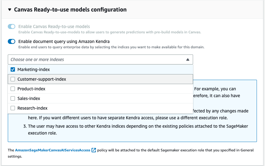
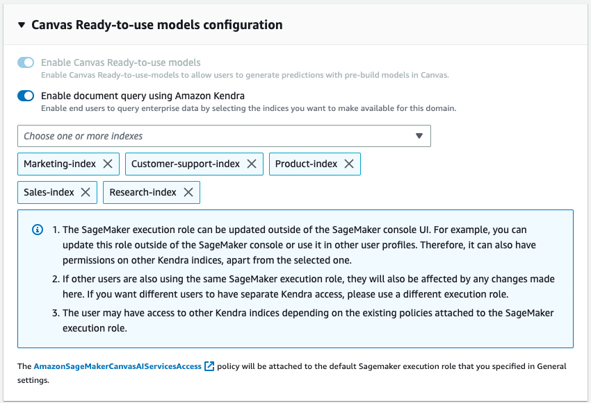
As part of the domain configuration, a cloud administrator can choose one or more Kendra indices that the business analyst can query when interacting with the FM through SageMaker Canvas.
After the Kendra indices are hydrated and configured, business analysts use them with SageMaker Canvas by starting a new chat and selecting “Query Documents” toggle. SageMaker Canvas will then manage the underlying communication between Amazon Kendra and the FM of choice to perform the following operations:
- Query the Kendra indices with the question coming from the user.
- Retrieve the snippets (and the sources) from Kendra indices.
- Engineer the prompt with the snippets with the original query so that the foundation model can generate an answer from the retrieved documents.
- Provide the generated answer to the user, along with references to the pages/documents that were used to formulate the response.
Setting up Canvas to query documents
In this section, we will walk you through the steps to set up Canvas to query documents served through Kendra indexes. You should have the following prerequisites:
- SageMaker Domain setup – Onboard to Amazon SageMaker Domain
- Create a Kendra index (or more than one)
- Setup the Kendra Amazon S3 connector – follow the Amazon S3 Connector – and upload PDF files and other documents to the Amazon S3 bucket associated with the Kendra index
- Setup IAM so that Canvas has the appropriate permissions, including those required for calling Amazon Bedrock and/or SageMaker endpoints – follow the Set-up Canvas Chat documentation
Now you can update the Domain so that it can access the desired indices. On the SageMaker console, for the given Domain, select Edit under the Domain Settings tab. Enable the toggle “Enable query documents with Amazon Kendra” which can be found at the Canvas Settings step. Once activated, choose one or more Kendra indices that you want to use with Canvas. Once activated, choose one or more Kendra indices that you want to use with Canvas.
That’s all that’s needed to configure Canvas query documents feature. Users can now jump into a chat within Canvas and start using the knowledge bases that have been attached to the Domain through the Kendra indexes. The maintainers of the knowledge-base can continue to update the source-of-truth and with the syncing capability in Kendra, the chat users will automatically be able to use the up-to-date information in a seamless manner.
Using the Query Documents feature for chat
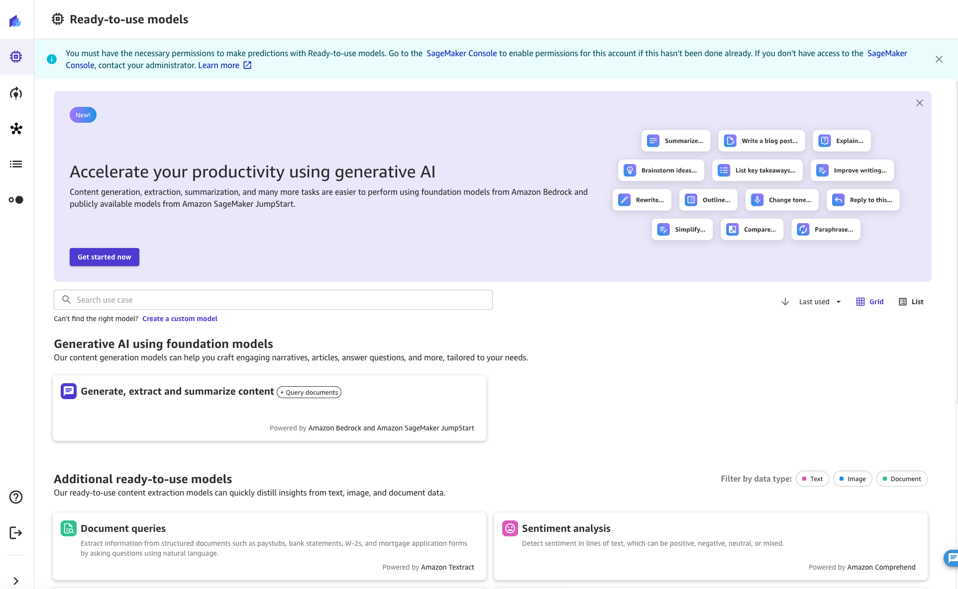
As a SageMaker Canvas user, the Query Documents feature can be accessed from within a chat. To start the chat session, click or search for the “Generate, extract and summarize content” button from the Ready-to-use models tab in SageMaker Canvas.
Once there, you can turn on and off Query Documents with the toggle at the top of the screen. Check out the information prompt to learn more about the feature.

When Query Documents is enabled, you can choose among a list of Kendra indices enabled by the cloud administrator.

You can select an index when starting a new chat. You can then ask a question in the UX with knowledge being automatically sourced from the selected index. Note that after a conversation has started against a specific index, it is not possible to switch to another index.

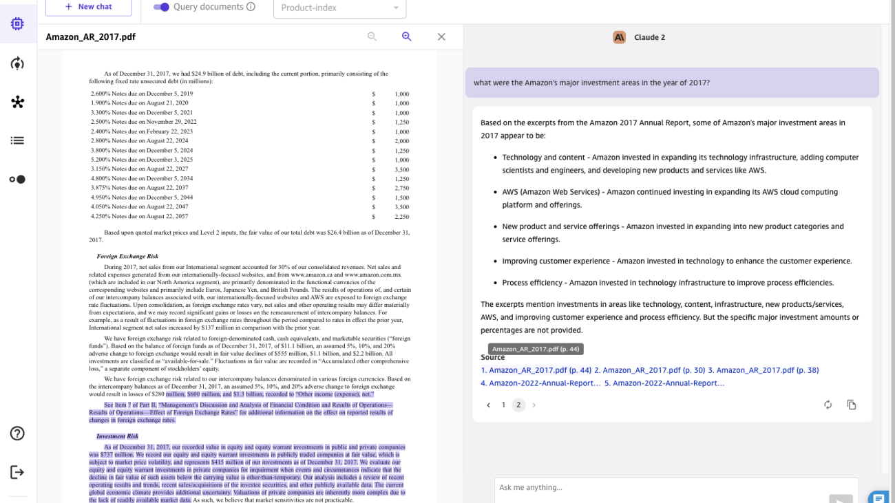
For the questions asked, the chat will show the answer generated by the FM along with the source documents that contributed to generating the answer. When clicking any of the source documents, Canvas opens a preview of the document, highlighting the excerpt used by the FM.

Conclusion
Conversational AI has immense potential to transform customer and employee experience by providing a human-like assistant with natural and intuitive interactions such as:
- Performing research on a topic or search and browse the organization’s knowledge base
- Summarizing volumes of content to rapidly gather insights
- Searching for Entities, Sentiments, PII and other useful data, and increasing the business value of unstructured content
- Generating drafts for documents and business correspondence
- Creating knowledge articles from disparate internal sources (incidents, chat logs, wikis)
The innovative integration of chat interfaces, knowledge retrieval, and FMs enables enterprises to provide accurate, relevant responses to user questions by using their domain knowledge and sources-of-truth.
By connecting SageMaker Canvas to knowledge bases in Amazon Kendra, organizations can keep their proprietary data within their own environment while still benefiting from state-of-the-art natural language capabilities of FMs. With the launch of SageMaker Canvas’s Query Documents feature, we are making it easy for any enterprise to use LLMs and their enterprise knowledge as source-of-truth to power a secure chat experience. All this functionality is available in a no-code format, allowing businesses to avoid handling the repetitive and non-specialized tasks.
To learn more about SageMaker Canvas and how it helps make it easier for everyone to start with Machine Learning, check out the SageMaker Canvas announcement. Learn more about how SageMaker Canvas helps foster collaboration between data scientists and business analysts by reading the Build, Share & Deploy post. Finally, to learn how to create your own Retrieval Augmented Generation workflow, refer to SageMaker JumpStart RAG.
References
Lewis, P., Perez, E., Piktus, A., Petroni, F., Karpukhin, V., Goyal, N., Küttler, H., Lewis, M., Yih, W., Rocktäschel, T., Riedel, S., Kiela, D. (2020). Retrieval-Augmented Generation for Knowledge-Intensive NLP Tasks. Advances in Neural Information Processing Systems, 33, 9459-9474.
About the Authors
 Davide Gallitelli is a Senior Specialist Solutions Architect for AI/ML. He is based in Brussels and works closely with customers all around the globe that are looking to adopt Low-Code/No-Code Machine Learning technologies, and Generative AI. He has been a developer since he was very young, starting to code at the age of 7. He started learning AI/ML at university, and has fallen in love with it since then.
 Bilal Alam is an Enterprise Solutions Architect at AWS with a focus on the Financial Services industry. On most days Bilal is helping customers with building, uplifting and securing their AWS environment to deploy their most critical workloads. He has extensive experience in Telco, networking, and software development. More recently, he has been looking into using AI/ML to solve business problems.
 Pashmeen Mistry is a Senior Product Manager at AWS. Outside of work, Pashmeen enjoys adventurous hikes, photography, and spending time with his family.
 Dan Sinnreich is a Senior Product Manager at AWS, helping to democratize low-code/no-code machine learning. Previous to AWS, Dan built and commercialized enterprise SaaS platforms and time-series models used by institutional investors to manage risk and construct optimal portfolios. Outside of work, he can be found playing hockey, scuba diving, and reading science fiction.

Turning the Tide on Coral Reef Decline: CUREE Robot Dives Deep With Deep Learning
Researchers are taking deep learning for a deep dive, literally.
The Woods Hole Oceanographic Institution (WHOI) Autonomous Robotics and Perception Laboratory (WARPLab) and MIT are developing a robot for studying coral reefs and their ecosystems.
The WARPLab autonomous underwater vehicle (AUV), enabled by an NVIDIA Jetson Orin NX module, is an effort from the world’s largest private ocean research institution to turn the tide on reef declines.
Some 25% of coral reefs worldwide have vanished in the past three decades, and most of the remaining reefs are heading for extinction, according to the WHOI Reef Solutions Initiative.
The AUV, dubbed CUREE (Curious Underwater Robot for Ecosystem Exploration), gathers visual, audio, and other environmental data alongside divers to help understand the human impact on reefs and the sea life around them. The robot runs an expanding collection of NVIDIA Jetson-enabled edge AI to build 3D models of reefs and to track creatures and plant life. It also runs models to navigate and collect data autonomously.
WHOI, whose submarine first explored the Titanic in 1986, is developing its CUREE robot for data gathering to scale the effort and aid in mitigation strategies. The oceanic research organization is also exploring the use of simulation and digital twins to better replicate reef conditions and investigate solutions like NVIDIA Omniverse, a development platform for building and connecting 3D tools and applications.
Creating a digital twin of Earth in Omniverse, NVIDIA is developing the world’s most powerful AI supercomputer for predicting climate change, called Earth-2.
Underwater AI: DeepSeeColor Model
Anyone who’s gone snorkeling knows that seeing underwater isn’t as clear as seeing on land. Over distance, water attenuates the visible spectrum of light from the sun underwater, muting some colors more than others. At the same time, particles in the water create a hazy view, known as backscatter.
A team from WARPLab recently published a research paper on undersea vision correction that helps mitigate these problems and supports the work of CUREE. The paper describes a model, called DeepSeeColor, that uses a sequence of two convolutional neural networks to reduce backscatter and correct colors in real time on the NVIDIA Jetson Orin NX while undersea.
“NVIDIA GPUs are involved in a large portion of our pipeline because, basically, when the images come in, we use DeepSeeColor to color correct them, and then we can do the fish detection and transmit that to a scientist up at the surface on a boat,” said Stewart Jamieson, a robotics Ph.D. candidate at MIT and AI developer at WARPLab.
Eyes and Ears: Fish and Reef Detection
CUREE packs four forward-facing cameras, four hydrophones for underwater audio capture, depth sensors and inertial measurement unit sensors. GPS doesn’t work underwater, so it is only used to initialize the robot’s starting position while on the surface.
Using a combination of cameras and hydrophones along with AI models running on the Jetson Orin NX enables CUREE to collect data for producing 3D models of reefs and undersea terrains.
To use the hydrophones for audio data collection, CUREE needs to drift with its motor off so that there’s no interference with the audio.
“It can build a spatial soundscape map of the reef, using sounds produced by different animals,” said Yogesh Girdhar, an associate scientist at WHOI, who leads WARPLab. “We currently (in post-processing) detect where all the chatter associated with bioactivity hotspots is,” he added, referring to all the noises of sea life.
The team has been training detection models for both audio and video input to track creatures. But a big noise interference with detecting clear audio samples has come from one creature in particular.
“The problem is that, underwater, the snapping shrimps are loud,” said Girdhar. On land, this classic dilemma of how to separate sounds from background noises is known as the cocktail party problem. “If only we could figure out an algorithm to remove the effects of sounds of snapping shrimps from audio, but at the moment we don’t have a good solution,” said Girdhar.
Despite few underwater datasets in existence, pioneering fish detection and tracking is going well, said Levi Cai, a Ph.D. candidate in the MIT-WHOI joint program. He said they’re taking a semi-supervised approach to the marine animal tracking problem. The tracking is initialized using targets detected by a fish detection neural network trained on open-source datasets for fish detection, which is fine-tuned with transfer learning from images gathered by CUREE.
“We manually drive the vehicle until we see an animal that we want to track, and then we click on it and have the semi-supervised tracker take over from there,” said Cai.
Jetson Orin Energy Efficiency Drives CUREE
Energy efficiency is critical for small AUVs like CUREE. The compute requirements for data collection consume roughly 25% of the available energy resources, with driving the robots taking the remainder.
CUREE typically operates for as long as two hours on a charge, depending on the reef mission and the observation requirements, said Girdhar, who goes on the dive missions in St. John in the U.S. Virgin Islands.
To enhance energy efficiency, the team is looking into AI for managing the sensors so that computing resources automatically stay awake while making observations and sleep when not in use.
“Our robot is small, so the amount of energy spent on GPU computing actually matters — with Jetson Orin NX our power issues are gone, and it’s made our system much more robust,” said Girdhar.
Exploring Isaac Sim to Make Improvements
The WARPLab team is experimenting with NVIDIA Isaac Sim, a scalable robotics simulation application and synthetic data generation tool powered by Omniverse, to accelerate development of autonomy and observation for CUREE.
The goal is to do simple simulations in Isaac Sim to get the core essence of the problem to be simulated and then finish the training in the real world undersea, said Yogesh.
“In a coral reef environment, we cannot depend on sonars — we need to get up really close,” he said. “Our goal is to observe different ecosystems and processes happening.”
Understanding Ecosystems and Creating Mitigation Strategies
The WARPLab team intends to make the CUREE platform available for others to understand the impact humans are having on undersea environments and to help create mitigation strategies.
The researchers plan to learn from patterns that emerge from the data. CUREE provides an almost fully autonomous data collection scientist that can communicate findings to human researchers, said Jamieson. “A scientist gets way more out of this than if the task had to be done manually, driving it around staring at a screen all day,” he said.
Girdhar said that ecosystems like coral reefs can be modeled with a network, with different nodes corresponding to different types of species and habitat types. Within that, he said, there are all these different interactions happening, and the researchers seek to understand this network to learn about the relationship between various animals and their habitats.
The hope is that there’s enough data collected using CUREE AUVs to gain a comprehensive understanding of ecosystems and how they might progress over time and be affected by harbors, pesticide runoff, carbon emissions and dive tourism, he said.
“We can then better design and deploy interventions and determine, for example, if we planted new corals how they would change the reef over time,” said Girdar.
Learn more about NVIDIA Jetson Orin NX, Omniverse and Earth-2.
Project Silica: Sustainable cloud archival storage in glass
This research paper was presented at the 29th ACM Symposium on Operating Systems Principles (opens in new tab) (SOSP 2023), the premier forum for the theory and practice of computer systems software.
Data growth demands a sustainable archival solution
For millennia, data has woven itself into every facet of our lives, from business and academia to personal spheres. Our production of data is staggering, encompassing personal photos, medical records, financial data, scientific insights, and more. By 2025, it’s estimated that we will generate a massive 175 zettabytes of data annually. Amidst this deluge, a substantial portion is vital for preserving our collective heritage and personal histories.
Presently, magnetic technologies like tape and hard disk drives provide the most economical storage, but they come with limitations. Magnetic media lacks the longevity and durability essential for enduring archival storage, requiring data to be periodically migrated to new media—for hard disk drives, this is every five years, for magnetic tape, it’s around ten. Moreover, ensuring data longevity on magnetic media requires regular “scrubbing,” a process involving reading data to identify corruption and fixing any errors. This leads to substantial energy consumption. We need a sustainable solution, one that ensures the preservation of our digital heritage without imposing an ongoing environmental and financial burden.
Project Silica: Sustainable and durable cloud archival storage
Our paper, “Project Silica: Towards Sustainable Cloud Archival Storage in Glass, (opens in new tab)” presented at SOSP 2023 (opens in new tab), describes Project Silica, a cloud-based storage system underpinned by quartz glass. This type of glass is a durable, chemically inert, and resilient low-cost media, impervious to electromagnetic interference. With data’s lifespan lasting thousands of years, quartz glass is ideal for archival storage, offering a sustainable solution and eliminating the need for periodic data refreshes.
Writing, reading, and decoding data
Ultrafast femtosecond lasers enable the writing process. Data is written inside a square glass platter similar in size to a DVD through voxels, permanent modifications to the physical structure of the glass made using femtosecond-scale laser pulses. Voxels encode multiple bits of data and are written in 2D layers across the XY plane. Hundreds of these layers are then stacked in the Z axis. To achieve high write throughput, we rapidly scan the laser pulses across the length of the media using a scanner similar to that used in barcode readers.
To read data, we employ polarization microscopy to image the platter. The read drive scans sectors in a single swift Z-pattern, and the resulting images are processed for decoding. Different read drive options offer varying throughput, balancing cost and performance.
Data decoding relies on ML models that analyze images captured by the read drive, accurately converting signals from analog to digital. The glass library design includes independent read, write, and storage racks. Platters are stored in power-free storage racks and moved by free-roaming shuttles, ensuring minimal resource consumption for passive storage, as shown in Video 1. A one-way system between write racks and the rest of the library ensures that a written platter cannot be over-written under any circumstances, enforcing data integrity.
Azure workload analysis informs Silica’s design
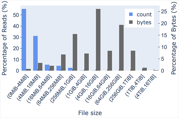
To build an optimal storage system around the core Silica technology, we extensively studied cloud archival data workloads from Azure Storage. Surprisingly, we discovered that small read requests dominate the read workload, yet a small percentage of requests constitute the majority of read bytes, creating a skewed distribution, as illustrated in Figure 1.
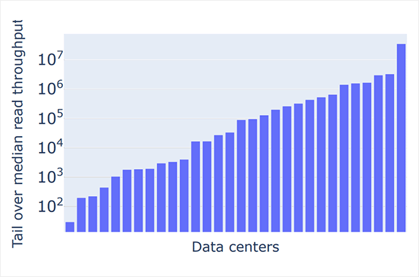
This implies that minimizing the latency of mechanical movement in the library is crucial for optimal performance. Silica glass, a random-seeking storage medium, can suitably meet these requirements as it eliminates the necessity for spooling, unlike magnetic tape. Figure 2 illustrates substantial differences in read demand across various datacenters. These results suggest that we need a flexible library design that can scale resources for each datacenter’s workload. Studying these archival workloads has been instrumental in helping us establish the core design principles for the Silica storage system.
Microsoft Research Podcast

Collaborators: Renewable energy storage with Bichlien Nguyen and David Kwabi
Dr. Bichlien Nguyen and Dr. David Kwabi explore their work in flow batteries and how machine learning can help more effectively search the vast organic chemistry space to identify compounds with properties just right for storing waterpower and other renewables.
Project Silica’s versatile storage system
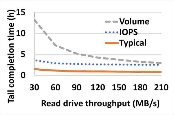
We designed and evaluated a comprehensive storage system that manages error correction, data layout, request scheduling, and shuttle traffic management. Our design effectively manages IOPS-intensive tasks, meeting the expected service level objective (SLO) of an archival storage tier, approximately 15 hours. Interestingly, even in volume-intensive scenarios where a large number of bytes are read, our system efficiently handles requests using read drives with low throughput. In both cases, throughput demands are significantly below those of traditional tape drives. This is shown in Figure 3. The paper provides an extensive description of this system, and the video above shows our prototype library’s capabilities.
Diverse applications for sustainably archiving humanity’s data
Project Silica holds promise in numerous sectors, such as healthcare, scientific research, and finance, where secure and durable archival storage of sensitive data is crucial. Research institutions could benefit from Silica’s ability to store vast datasets generated from experiments and simulations, ensuring the integrity and accessibility of research findings over time. Similarly, healthcare organizations could securely archive patient records, medical imaging data, and research outcomes for long-term reference and analysis.
As the volume of globally generated data grows, traditional storage solutions will continue to face challenges in terms of scalability, energy-efficiency, and long-term durability. Moreover, as technologies like AI and advanced analytics progress, the need for reliable and accessible archival data will continue to intensify. Project Silica is well-positioned to play a pivotal role in supporting these technologies by providing a stable, secure, and sustainable repository for the vast amounts of data we create and rely on.
The post Project Silica: Sustainable cloud archival storage in glass appeared first on Microsoft Research.

Spoken question answering and speech continuation using a spectrogram-powered LLM
The goal of natural language processing (NLP) is to develop computational models that can understand and generate natural language. By capturing the statistical patterns and structures of text-based natural language, language models can predict and generate coherent and meaningful sequences of words. Enabled by the increasing use of the highly successful Transformer model architecture and with training on large amounts of text (with proportionate compute and model size), large language models (LLMs) have demonstrated remarkable success in NLP tasks.
However, modeling spoken human language remains a challenging frontier. Spoken dialog systems have conventionally been built as a cascade of automatic speech recognition (ASR), natural language understanding (NLU), response generation, and text-to-speech (TTS) systems. However, to date there have been few capable end-to-end systems for the modeling of spoken language: i.e., single models that can take speech inputs and generate its continuation as speech outputs.
Today we present a new approach for spoken language modeling, called Spectron, published in “Spoken Question Answering and Speech Continuation Using Spectrogram-Powered LLM.” Spectron is the first spoken language model that is trained end-to-end to directly process spectrograms as both input and output, instead of learning discrete speech representations. Using only a pre-trained text language model, it can be fine-tuned to generate high-quality, semantically accurate spoken language. Furthermore, the proposed model improves upon direct initialization in retaining the knowledge of the original LLM as demonstrated through spoken question answering datasets.
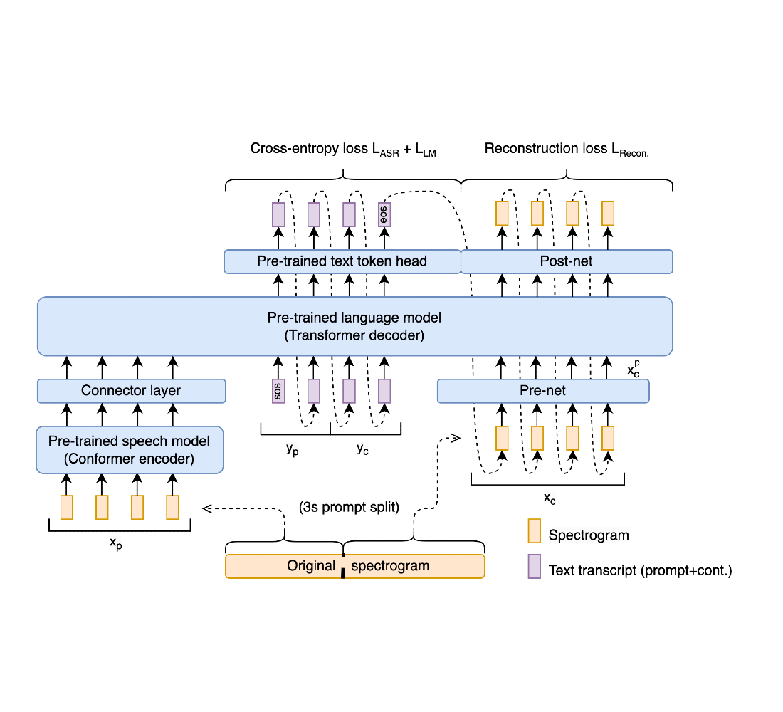
We show that a pre-trained speech encoder and a language model decoder enable end-to-end training and state-of-the-art performance without sacrificing representational fidelity. Key to this is a novel end-to-end training objective that implicitly supervises speech recognition, text continuation, and conditional speech synthesis in a joint manner. A new spectrogram regression loss also supervises the model to match the higher-order derivatives of the spectrogram in the time and frequency domain. These derivatives express information aggregated from multiple frames at once. Thus, they express rich, longer-range information about the shape of the signal. Our overall scheme is summarized in the following figure:
 |
| The Spectron model connects the encoder of a speech recognition model with a pre-trained Transformer-based decoder language model. At training, speech utterances split into a prompt and its continuation. Then the full transcript (prompt and continuation) is reconstructed along with the continuation’s speech features. At inference, only a prompt is provided; the prompt’s transcription, text continuation, and speech continuations are all generated by the model. |
Spectron architecture
The architecture is initialized with a pre-trained speech encoder and a pre-trained decoder language model. The encoder is prompted with a speech utterance as input, which it encodes into continuous linguistic features. These features feed into the decoder as a prefix, and the whole encoder-decoder is optimized to jointly minimize a cross-entropy loss (for speech recognition and transcript continuation) and a novel reconstruction loss (for speech continuation). During inference, one provides a spoken speech prompt, which is encoded and then decoded to give both text and speech continuations.
Speech encoder
The speech encoder is a 600M-parameter conformer encoder pre-trained on large-scale data (12M hours). It takes the spectrogram of the source speech as input, generating a hidden representation that incorporates both linguistic and acoustic information. The input spectrogram is first subsampled using a convolutional layer and then processed by a series of conformer blocks. Each conformer block consists of a feed-forward layer, a self-attention layer, a convolution layer, and a second feed-forward layer. The outputs are passed through a projection layer to match the hidden representations to the embedding dimension of the language model.
Language model
We use a 350M or 1B parameter decoder language model (for the continuation and question-answering tasks, respectively) trained in the manner of PaLM 2. The model receives the encoded features of the prompt as a prefix. Note that this is the only connection between the speech encoder and the LM decoder; i.e., there is no cross-attention between the encoder and the decoder. Unlike most spoken language models, during training, the decoder is teacher-forced to predict the text transcription, text continuation, and speech embeddings. To convert the speech embeddings to and from spectrograms, we introduce lightweight modules pre- and post-network.
By having the same architecture decode the intermediate text and the spectrograms, we gain two benefits. First, the pre-training of the LM in the text domain allows continuation of the prompt in the text domain before synthesizing the speech. Secondly, the predicted text serves as intermediate reasoning, enhancing the quality of the synthesized speech, analogous to improvements in text-based language models when using intermediate scratchpads or chain-of-thought (CoT) reasoning.
Acoustic projection layers
To enable the language model decoder to model spectrogram frames, we employ a multi-layer perceptron “pre-net” to project the ground truth spectrogram speech continuations to the language model dimension. This pre-net compresses the spectrogram input into a lower dimension, creating a bottleneck that aids the decoding process. This bottleneck mechanism prevents the model from repetitively generating the same prediction in the decoding process. To project the LM output from the language model dimension to the spectrogram dimension, the model employs a “post-net”, which is also a multi-layer perceptron. Both pre- and post-networks are two-layer multi-layer perceptrons.
Training objective
The training methodology of Spectron uses two distinct loss functions: (i) cross-entropy loss, employed for both speech recognition and transcript continuation, and (ii) regression loss, employed for speech continuation. During training, all parameters are updated (speech encoder, projection layer, LM, pre-net, and post-net).
Audio samples
Following are examples of speech continuation and question answering from Spectron:
Speech Continuation |
|
| Prompt: | |
| Continuation: | |
| Prompt: | |
| Continuation: | |
| Prompt: | |
| Continuation: | |
| Prompt: | |
| Continuation: | |
Question Answering |
|
| Question: | |
| Answer: | |
| Question: | |
| Answer: | |
Performance
To empirically evaluate the performance of the proposed approach, we conducted experiments on the Libri-Light dataset. Libri-Light is a 60k hour English dataset consisting of unlabelled speech readings from LibriVox audiobooks. We utilized a frozen neural vocoder called WaveFit to convert the predicted spectrograms into raw audio. We experiment with two tasks, speech continuation and spoken question answering (QA). Speech continuation quality is tested on the LibriSpeech test set. Spoken QA is tested on the Spoken WebQuestions datasets and a new test set named LLama questions, which we created. For all experiments, we use a 3 second audio prompt as input. We compare our method against existing spoken language models: AudioLM, GSLM, TWIST and SpeechGPT. For the speech continuation task, we use the 350M parameter version of LM and the 1B version for the spoken QA task.
For the speech continuation task, we evaluate our method using three metrics. The first is log-perplexity, which uses an LM to evaluate the cohesion and semantic quality of the generated speech. The second is mean opinion score (MOS), which measures how natural the speech sounds to human evaluators. The third, speaker similarity, uses a speaker encoder to measure how similar the speaker in the output is to the speaker in the input. Performance in all 3 metrics can be seen in the following graphs.
 |
| Log-perplexity for completions of LibriSpeech utterances given a 3-second prompt. Lower is better. |
 |
| Speaker similarity between the prompt speech and the generated speech using the speaker encoder. Higher is better. |
 |
| MOS given by human users on speech naturalness. Raters rate 5-scale subjective mean opinion score (MOS) ranging between 0 – 5 in naturalness given a speech utterance. Higher is better. |
As can be seen in the first graph, our method significantly outperforms GSLM and TWIST on the log-perplexity metric, and does slightly better than state-of-the-art methods AudioLM and SpeechGPT. In terms of MOS, Spectron exceeds the performance of all the other methods except for AudioLM. In terms of speaker similarity, our method outperforms all other methods.
To evaluate the ability of the models to perform question answering, we use two spoken question answering datasets. The first is the LLama Questions dataset, which uses general knowledge questions in different domains generated using the LLama2 70B LLM. The second dataset is the WebQuestions dataset which is a general question answering dataset. For evaluation we use only questions that fit into the 3 second prompt length. To compute accuracy, answers are transcribed and compared to the ground truth answers in text form.
 |
| Accuracy for Question Answering on the LLama Questions and Spoken WebQuestions datasets. Accuracy is computed using the ASR transcripts of spoken answers. |
First, we observe that all methods have more difficulty answering questions from the Spoken WebQuestions dataset than from the LLama questions dataset. Second, we observe that methods centered around spoken language modeling such as GSLM, AudioLM and TWIST have a completion-centric behavior rather than direct question answering which hindered their ability to perform QA. On the LLama questions dataset our method outperforms all other methods, while SpeechGPT is very close in performance. On the Spoken WebQuestions dataset, our method outperforms all other methods except for SpeechGPT, which does marginally better.
Acknowledgements
The direct contributors to this work include Eliya Nachmani, Alon Levkovitch, Julian Salazar, Chulayutsh Asawaroengchai, Soroosh Mariooryad, RJ Skerry-Ryan and Michelle Tadmor Ramanovich. We also thank Heiga Zhen, Yifan Ding, Yu Zhang, Yuma Koizumi, Neil Zeghidour, Christian Frank, Marco Tagliasacchi, Nadav Bar, Benny Schlesinger and Blaise Aguera-Arcas.