Monthly Archives: November 2023

Creating high-performance machine learning (ML) solutions relies on exploring and optimizing training parameters, also known as hyperparameters. Hyperparameters are the knobs and levers that we use to adjust the training process, such as learning rate, batch size, regularization strength, and others, depending on the specific model and task at hand. Exploring hyperparameters involves systematically varying the values of each parameter and observing the impact on model performance. Although this process requires additional efforts, the benefits are significant. Hyperparameter optimization (HPO) can lead to faster training times, improved model accuracy, and better generalization to new data.

We continue our journey from the post Optimize hyperparameters with Amazon SageMaker Automatic Model Tuning. We previously explored a single job optimization, visualized the outcomes for SageMaker built-in algorithm, and learned about the impact of particular hyperparameter values. On top of using HPO as a one-time optimization at the end of the model creation cycle, we can also use it across multiple steps in a conversational manner. Each tuning job helps us get closer to a good performance, but additionally, we also learn how sensitive the model is to certain hyperparameters and can use this understanding to inform the next tuning job. We can revise the hyperparameters and their value ranges based on what we learned and therefore turn this optimization effort into a conversation. And in the same way that we as ML practitioners accumulate knowledge over these runs, Amazon SageMaker Automatic Model Tuning (AMT) with warm starts can maintain this knowledge acquired in previous tuning jobs for the next tuning job as well.

In this post, we run multiple HPO jobs with a custom training algorithm and different HPO strategies such as Bayesian optimization and random search. We also put warm starts into action and visually compare our trials to refine hyperparameter space exploration.

Advanced concepts of SageMaker AMT

In the next sections, we take a closer look at each of the following topics and show how SageMaker AMT can help you implement them in your ML projects:

• Use custom training code and the popular ML framework Scikit-learn in SageMaker Training
• Define custom evaluation metrics based on the logs for evaluation and optimization
• Perform HPO using an appropriate strategy
• Use warm starts to turn a single hyperparameter search into a dialog with our model
• Use advanced visualization techniques using our solution library to compare two HPO strategies and tuning jobs results

Whether you’re using the built-in algorithms used in our first post or your own training code, SageMaker AMT offers a seamless user experience for optimizing ML models. It provides key functionality that allows you to focus on the ML problem at hand while automatically keeping track of the trials and results. At the same time, it automatically manages the underlying infrastructure for you.

In this post, we move away from a SageMaker built-in algorithm and use custom code. We use a Random Forest from SkLearn. But we stick to the same ML task and dataset as in our first post, which is detecting handwritten digits. We cover the content of the Jupyter notebook 2_advanced_tuning_with_custom_training_and_visualizing.ipynb and invite you to invoke the code side by side to read further.

Let’s dive deeper and discover how we can use custom training code, deploy it, and run it, while exploring the hyperparameter search space to optimize our results.

How to build an ML model and perform hyperparameter optimization

What does a typical process for building an ML solution look like? Although there are many possible use cases and a large variety of ML tasks out there, we suggest the following mental model for a stepwise approach:

1. Understand your ML scenario at hand and select an algorithm based on the requirements. For example, you might want to solve an image recognition task using a supervised learning algorithm. In this post, we continue to use the handwritten image recognition scenario and the same dataset as in our first post.
2. Decide which implementation of the algorithm in SageMaker Training you want to use. There are various options, inside SageMaker or external ones. Additionally, you need to define which underlying metric fits best for your task and you want to optimize for (such as accuracy, F1 score, or ROC). SageMaker supports four options depending on your needs and resources:
   • Use a pre-trained model via Amazon SageMaker JumpStart, which you can use out of the box or just fine-tune it.
   • Use one of the built-in algorithms for training and tuning, like XGBoost, as we did in our previous post.
   • Train and tune a custom model based on one of the major frameworks like Scikit-learn, TensorFlow, or PyTorch. AWS provides a selection of pre-made Docker images for this purpose. For this post, we use this option, which allows you to experiment quickly by running your own code on top of a pre-made container image.
   • Bring your own custom Docker image in case you want to use a framework or software that is not otherwise supported. This option requires the most effort, but also provides the highest degree of flexibility and control.
3. Train the model with your data. Depending on the algorithm implementation from the previous step, this can be as simple as referencing your training data and running the training job or by additionally providing custom code for training. In our case, we use some custom training code in Python based on Scikit-learn.
4. Apply hyperparameter optimization (as a “conversation” with your ML model). After the training, you typically want to optimize the performance of your model by finding the most promising combination of values for your algorithm’s hyperparameters.

Depending on your ML algorithm and model size, the last step of hyperparameter optimization may turn out to be a bigger challenge than expected. The following questions are typical for ML practitioners at this stage and might sound familiar to you:

• What kind of hyperparameters are impactful for my ML problem?
• How can I effectively search a huge hyperparameter space to find those best-performing values?
• How does the combination of certain hyperparameter values influence my performance metric?
• Costs matter; how can I use my resources in an efficient manner?
• What kind of tuning experiments are worthwhile, and how can I compare them?

It’s not easy to answer these questions, but there is good news. SageMaker AMT takes the heavy lifting from you, and lets you concentrate on choosing the right HPO strategy and value ranges you want to explore. Additionally, our visualization solution facilitates the iterative analysis and experimentation process to efficiently find well-performing hyperparameter values.

In the next sections, we build a digit recognition model from scratch using Scikit-learn and show all these concepts in action.

Solution overview

SageMaker offers some very handy features to train, evaluate, and tune our model. It covers all functionality of an end-to-end ML lifecycle, so we don’t even need to leave our Jupyter notebook.

In our first post, we used the SageMaker built-in algorithm XGBoost. For demonstration purposes, this time we switch to a Random Forest classifier because we can then show how to provide your own training code. We opted for providing our own Python script and using Scikit-learn as our framework. Now, how do we express that we want to use a specific ML framework? As we will see, SageMaker uses another AWS service in the background to retrieve a pre-built Docker container image for training—Amazon Elastic Container Registry (Amazon ECR).

We cover the following steps in detail, including code snippets and diagrams to connect the dots. As mentioned before, if you have the chance, open the notebook and run the code cells step by step to create the artifacts in your AWS environment. There is no better way of active learning.

1. First, load and prepare the data. We use Amazon Simple Storage Service (Amazon S3) to upload a file containing our handwritten digits data.
2. Next, prepare the training script and framework dependencies. We provide the custom training code in Python, reference some dependent libraries, and make a test run.
3. To define the custom objective metrics, SageMaker lets us define a regular expression to extract the metrics we need from the container log files.
4. Train the model using the scikit-learn framework. By referencing a pre-built container image, we create a corresponding Estimator object and pass our custom training script.
5. AMT enables us to try out various HPO strategies. We concentrate on two of them for this post: random search and Bayesian search.
6. Choose between SageMaker HPO strategies.
7. Visualize, analyze, and compare tuning results. Our visualization package allows us to discover which strategy performs better and which hyperparameter values deliver the best performance based on our metrics.
8. Continue the exploration of the hyperparameter space and warm start HPO jobs.

AMT takes care of scaling and managing the underlying compute infrastructure to run the various tuning jobs on Amazon Elastic Compute Cloud (Amazon EC2) instances. This way, you don’t need to burden yourself to provision instances, handle any operating system and hardware issues, or aggregate log files on your own. The ML framework image is retrieved from Amazon ECR and the model artifacts including tuning results are stored in Amazon S3. All logs and metrics are collected in Amazon CloudWatch for convenient access and further analysis if needed.

Prerequisites

Because this is a continuation of a series, it is recommended, but not necessarily required, to read our first post about SageMaker AMT and HPO. Apart from that, basic familiarity with ML concepts and Python programming is helpful. We also recommend following along with each step in the accompanying notebook from our GitHub repository while reading this post. The notebook can be run independently from the first one, but needs some code from subfolders. Make sure to clone the full repository in your environment as described in the README file.

Experimenting with the code and using the interactive visualization options greatly enhances your learning experience. So, please check it out.

Load and prepare the data

As a first step, we make sure the downloaded digits data we need for training is accessible to SageMaker. Amazon S3 allows us to do this in a safe and scalable way. Refer to the notebook for the complete source code and feel free to adapt it with your own data.

sm_sess = sagemaker.session.Session(boto_session=boto_sess, sagemaker_client=sm)
BUCKET = sm_sess.default_bucket()
PREFIX = 'amt-visualize-demo'
s3_data_url = f's3://{BUCKET}/{PREFIX}/data'
digits         = datasets.load_digits()
digits_df      = pd.DataFrame(digits.data)
digits_df['y'] = digits.target
digits_df.to_csv('data/digits.csv', index=False)
!aws s3 sync data/ {s3_data_url} —exclude '*' —include 'digits.csv'

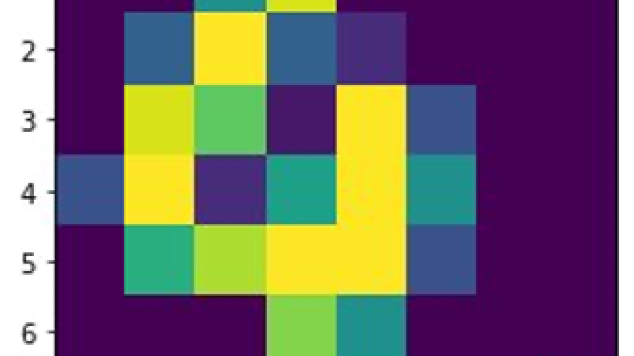
The digits.csv file contains feature data and labels. Each digit is represented by pixel values in an 8×8 image, as depicted by the following image for the digit 4.

Prepare the training script and framework dependencies

Now that the data is stored in our S3 bucket, we can define our custom training script based on Scikit-learn in Python. SageMaker gives us the option to simply reference the Python file later for training. Any dependencies like the Scikit-learn or pandas libraries can be provided in two ways:

• They can be specified explicitly in a requirements.txt file
• They are pre-installed in the underlying ML container image, which is either provided by SageMaker or custom-built

Both options are generally considered standard ways for dependency management, so you might already be familiar with it. SageMaker supports a variety of ML frameworks in a ready-to-use managed environment. This includes many of the most popular data science and ML frameworks like PyTorch, TensorFlow, or Scikit-learn, as in our case. We don’t use an additional requirements.txt file, but feel free to add some libraries to try it out.

The code of our implementation contains a method called fit(), which creates a new classifier for the digit recognition task and trains it. In contrast to our first post where we used the SageMaker built-in XGBoost algorithm, we now use a RandomForestClassifier provided by the ML library sklearn. The call of the fit() method on the classifier object starts the training process using a subset (80%) of our CSV data:

def fit(train_dir, n_estimators, max_depth, min_samples_leaf, max_features, min_weight_fraction_leaf):
    
    digits = pd.read_csv(Path(train_dir)/'digits.csv')
    
    Xtrain, Xtest, ytrain, ytest = train_test_split(digits.iloc[:, :-1], digits.iloc[:, -1], test_size=.2)
    
    m = RandomForestClassifier(n_estimators=n_estimators, 
                               max_depth=max_depth, 
                               min_samples_leaf=min_samples_leaf,
                               max_features=max_features,
                               min_weight_fraction_leaf=min_weight_fraction_leaf)
    m.fit(Xtrain, ytrain)
    predicted = m.predict(Xtest)
    pre, rec, f1, _ = precision_recall_fscore_support(ytest, predicted, pos_label=1, average='weighted')
    
    print(f'pre: {pre:5.3f} rec: {rec:5.3f} f1: {f1:5.3}')
    
    return m

See the full script in our Jupyter notebook on GitHub.

Before you spin up container resources for the full training process, did you try to run the script directly? This is a good practice to quickly ensure the code has no syntax errors, check for matching dimensions of your data structures, and some other errors early on.

There are two ways to run your code locally. First, you can run it right away in the notebook, which also allows you to use the Python Debugger pdb:

# Running the code from within the notebook. It would then be possible to use the Python Debugger, pdb.
from train import fit
fit('data', 100, 10, 1, 'auto', 0.01)

Alternatively, run the train script from the command line in the same way you may want to use it in a container. This also supports setting various parameters and overwriting the default values as needed, for example:

!cd src && python train.py --train ../data/ --model-dir /tmp/ --n-estimators 100

As output, you can see the first results for the model’s performance based on the objective metrics precision, recall, and F1-score. For example, pre: 0.970 rec: 0.969 f1: 0.969.

Not bad for such a quick training. But where did these numbers come from and what do we do with them?

Define custom objective metrics

Remember, our goal is to fully train and tune our model based on the objective metrics we consider relevant for our task. Because we use a custom training script, we need to define those metrics for SageMaker explicitly.

Our script emits the metrics precision, recall, and F1-score during training simply by using the print function:

print(f'pre: {pre:5.3f} rec: {rec:5.3f} f1: {f1:5.3}')

The standard output is captured by SageMaker and sent to CloudWatch as a log stream. To retrieve the metric values and work with them later in SageMaker AMT, we need to provide some information on how to parse that output. We can achieve this by defining regular expression statements (for more information, refer to Monitor and Analyze Training Jobs Using Amazon CloudWatch Metrics):

metric_definitions = [
    {'Name': 'valid-precision',  'Regex': r'pre:s+(-?[0-9.]+)'},
    {'Name': 'valid-recall',     'Regex': r'rec:s+(-?[0-9.]+)'},
    {'Name': 'valid-f1',         'Regex': r'f1:s+(-?[0-9.]+)'}]   

Let’s walk through the first metric definition in the preceding code together. SageMaker will look for output in the log that starts with pre: and is followed by one or more whitespace and then a number that we want to extract, which is why we use the round parenthesis. Every time SageMaker finds a value like that, it turns it into a CloudWatch metric with the name valid-precision.

Train the model using the Scikit-learn framework

After we create our training script train.py and instruct SageMaker on how to monitor the metrics within CloudWatch, we define a SageMaker Estimator object. It initiates the training job and uses the instance type we specify. But how can this instance type be different from the one you run an Amazon SageMaker Studio notebook on, and why? SageMaker Studio runs your training (and inference) jobs on separate compute instances than your notebook. This allows you to continue working in your notebook while the jobs run in the background.

The parameter framework_version refers to the Scikit-learn version we use for our training job. Alternatively, we can pass image_uri to the estimator. You can check whether your favorite framework or ML library is available as a pre-built SageMaker Docker image and use it as is or with extensions.

Moreover, we can run SageMaker training jobs on EC2 Spot Instances by setting use_spot_instances to True. They are spare capacity instances that can save up to 90% of costs.  These instances provide flexibility on when the training jobs are run.

estimator = SKLearn(
    'train.py',
    source_dir='src',
    role=get_execution_role(),
    instance_type= 'ml.m5.large',
    instance_count=1,
    framework_version='0.23-1',
    metric_definitions=metric_definitions,

    # Uncomment the following three lines to use Managed Spot Training
    # use_spot_instances= True,
    # max_run=  60 * 60 * 24,
    # max_wait= 60 * 60 * 24,

    hyperparameters = {'n-estimators': 100,
                       'max-depth': 10,
                       'min-samples-leaf': 1,
                       'max-features': 'auto',
                       'min-weight-fraction-leaf': 0.1}
)

After the Estimator object is set up, we start the training by calling the fit() function, supplying the path to the training dataset on Amazon S3. We can use this same method to provide validation and test data. We set the wait parameter to True so we can use the trained model in the subsequent code cells.

estimator.fit({'train': s3_data_url}, wait=True)

Define hyperparameters and run tuning jobs

So far, we have trained the model with one set of hyperparameter values. But were those values good? Or could we look for better ones? Let’s use the HyperparameterTuner class to run a systematic search over the hyperparameter space. How do we search this space with the tuner? The necessary parameters are the objective metric name and objective type that will guide the optimization. The optimization strategy is another key argument for the tuner because it further defines the search space. The following are four different strategies to choose from:

• Grid search
• Random search
• Bayesian optimization (default)
• Hyperband

We further describe these strategies and equip you with some guidance to choose one later in this post.

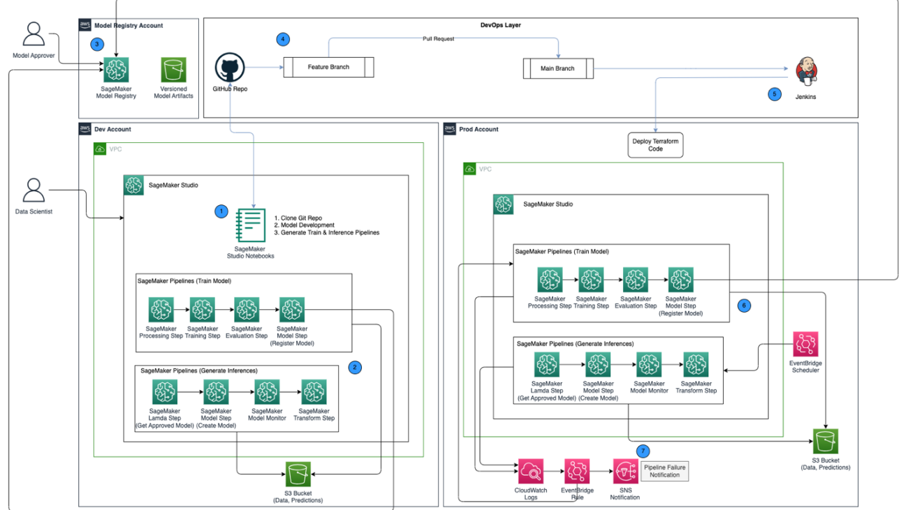
Before we define and run our tuner object, let’s recap our understanding from an architecture perspective. We covered the architectural overview of SageMaker AMT in our last post and reproduce an excerpt of it here for convenience.

We can choose what hyperparameters we want to tune or leave static. For dynamic hyperparameters, we provide hyperparameter_ranges that can be used to optimize for tunable hyperparameters. Because we use a Random Forest classifier, we have utilized the hyperparameters from the Scikit-learn Random Forest documentation.

We also limit resources with the maximum number of training jobs and parallel training jobs the tuner can use. We will see how these limits help us compare the results of various strategies with each other.

tuner_parameters = {
    'estimator': estimator,
    'base_tuning_job_name': 'random',
    'metric_definitions': metric_definitions,
    'objective_metric_name': 'valid-f1',
    'objective_type': 'Maximize',
    'hyperparameter_ranges': hpt_ranges,
    'strategy': 'Random',
    'max_jobs': n, # 50
    'max_parallel_jobs': k # 2
    } 

Similar to the Estimator’s fit function, we start a tuning job calling the tuner’s fit:

random_tuner = HyperparameterTuner(**tuner_parameters)
random_tuner.fit({'train': s3_data_url}, wait=False)

This is all we have to do to let SageMaker run the training jobs (n=50) in the background, each using a different set of hyperparameters. We explore the results later in this post. But before that, let’s start another tuning job, this time applying the Bayesian optimization strategy. We will compare both strategies visually after their completion.

tuner_parameters['strategy']             = 'Bayesian'
tuner_parameters['base_tuning_job_name'] = 'bayesian'
bayesian_tuner = HyperparameterTuner(**tuner_parameters)
bayesian_tuner.fit({'train': s3_data_url}, wait=False)

Note that both tuner jobs can run in parallel because SageMaker orchestrates the required compute instances independently of each other. That’s quite helpful for practitioners who experiment with different approaches at the same time, like we do here.

Choose between SageMaker HPO strategies

When it comes to tuning strategies, you have a few options with SageMaker AMT: grid search, random search, Bayesian optimization, and Hyperband. These strategies determine how the automatic tuning algorithms explore the specified ranges of hyperparameters.

Random search is pretty straightforward. It randomly selects combinations of values from the specified ranges and can be run in a sequential or parallel manner. It’s like throwing darts blindfolded, hoping to hit the target. We have started with this strategy, but will the results improve with another one?

Bayesian optimization takes a different approach than random search. It considers the history of previous selections and chooses values that are likely to yield the best results. If you want to learn from previous explorations, you can achieve this only with running a new tuning job after the previous ones. Makes sense, right? In this way, Bayesian optimization is dependent on the previous runs. But do you see what HPO strategy allows for higher parallelization?

Hyperband is an interesting one! It uses a multi-fidelity strategy, which means it dynamically allocates resources to the most promising training jobs and stops those that are underperforming. Therefore, Hyperband is computationally efficient with resources, learning from previous training jobs. After stopping the underperforming configurations, a new configuration starts, and its values are chosen randomly.

Depending on your needs and the nature of your model, you can choose between random search, Bayesian optimization, or Hyperband as your tuning strategy. Each has its own approach and advantages, so it’s important to consider which one works best for your ML exploration. The good news for ML practitioners is that you can select the best HPO strategy by visually comparing the impact of each trial on the objective metric. In the next section, we see how to visually identify the impact of different strategies.

Visualize, analyze, and compare tuning results

When our tuning jobs are complete, it gets exciting. What results do they deliver? What kind of boost can you expect on our metric compared to your base model? What are the best-performing hyperparameters for our use case?

A quick and straightforward way to view the HPO results is by visiting the SageMaker console. Under Hyperparameter tuning jobs, we can see (per tuning job) the combination of hyperparameter values that have been tested and delivered the best performance as measured by our objective metric (valid-f1).

Is that all you need? As an ML practitioner, you may be not only interested in those values, but certainly want to learn more about the inner workings of your model to explore its full potential and strengthen your intuition with empirical feedback.

A good visualization tool can greatly help you understand the improvement by HPO over time and get empirical feedback on design decisions of your ML model. It shows the impact of each individual hyperparameter on your objective metric and provides guidance to further optimize your tuning results.

We use the amtviz custom visualization package to visualize and analyze tuning jobs. It’s straightforward to use and provides helpful features. We demonstrate its benefit by interpreting some individual charts, and finally comparing random search side by side with Bayesian optimization.

First, let’s create a visualization for random search. We can do this by calling visualize_tuning_job() from amtviz and passing our first tuner object as an argument:

from amtviz import visualize_tuning_job
visualize_tuning_job(random_tuner, advanced=True, trials_only=True)

You will see a couple of charts, but let’s take it step by step. The first scatter plot from the output looks like the following and already gives us some visual clues we wouldn’t recognize in any table.

Each dot represents the performance of an individual training job (our objective valid-f1 on the y-axis) based on its start time (x-axis), produced by a specific set of hyperparameters. Therefore, we look at the performance of our model as it progresses over the duration of the tuning job.

The dotted line highlights the best result found so far and indicates improvement over time. The best two training jobs achieved an F1 score of around 0.91.

Besides the dotted line showing the cumulative progress, do you see a trend in the chart?

Probably not. And this is expected, because we’re viewing the results of the random HPO strategy. Each training job was run using a different but randomly selected set of hyperparameters. If we continued our tuning job (or ran another one with the same setting), we would probably see some better results over time, but we can’t be sure. Randomness is a tricky thing.

The next charts help you gauge the influence of hyperparameters on the overall performance. All hyperparameters are visualized, but for the sake of brevity, we focus on two of them: n-estimators and max-depth.

Our top two training jobs were using n-estimators of around 20 and 80, and max-depth of around 10 and 18, respectively. The exact hyperparameter values are displayed via tooltip for each dot (training job). They are even dynamically highlighted across all charts and give you a multi-dimensional view! Did you see that? Each hyperparameter is plotted against the objective metric, as a separate chart.

Now, what kind of insights do we get about n-estimators?

Based on the left chart, it seems that very low value ranges (below 10) more often deliver poor results compared to higher values. Therefore, higher values may help your model to perform better—interesting.

In contrast, the correlation of the max-depth hyperparameter to our objective metric is rather low. We can’t clearly tell which value ranges are performing better from a general perspective.

In summary, random search can help you find a well-performing set of hyperparameters even in a relatively short amount of time. Also, it isn’t biased towards a good solution but gives a balanced view of the search space. Your resource utilization, however, might not be very efficient. It continues to run training jobs with hyperparameters in value ranges that are known to deliver poor results.

Let’s examine the results of our second tuning job using Bayesian optimization. We can use amtviz to visualize the results in the same way as we did so far for the random search tuner. Or, even better, we can use the capability of the function to compare both tuning jobs in a single set of charts. Quite handy!

visualize_tuning_job([random_tuner, bayesian_tuner], advanced=True, trials_only=True)

There are more dots now because we visualize the results of all training jobs for both, the random search (orange dots) and the Bayesian optimization (blue dots). On the right side, you can see a density chart visualizing the distribution of all F1-scores. A majority of the training jobs achieved results in the upper part of the F1 scale (over 0.6)—that’s good!

What is the key takeaway here? The scatter plot clearly shows the benefit of Bayesian optimization. It delivers better results over time because it can learn from previous runs. That’s why we achieved significantly better results using Bayesian compared to random (0.967 vs. 0.919) with the same number of training jobs.

There is even more you can do with amtviz. Let’s drill in.

If you give SageMaker AMT the instruction to run a larger number of jobs for tuning, seeing many trials at once can get messy. That’s one of the reasons why we made these charts interactive. You can click and drag on every hyperparameter scatter plot to zoom in to certain value ranges and refine your visual interpretation of the results. All other charts are automatically updated. That’s pretty helpful, isn’t it? See the next charts as an example and try it for yourself in your notebook!

As a tuning maximalist, you may also decide that running another hyperparameter tuning job could further improve your model performance. But this time, a more specific range of hyperparameter values can be explored because you already know (roughly) where to expect better results. For example, you may choose to focus on values between 100–200 for n-estimators, as shown in the chart. This lets AMT focus on the most promising training jobs and increases your tuning efficiency.

To sum it up, amtviz provides you with a rich set of visualization capabilities that allow you to better understand the impact of your model’s hyperparameters on performance and enable smarter decisions in your tuning activities.

Continue the exploration of the hyperparameter space and warm start HPO jobs

We have seen that AMT helps us explore the hyperparameter search space efficiently. But what if we need multiple rounds of tuning to iteratively improve our results? As mentioned in the beginning, we want to establish an optimization feedback cycle—our “conversation” with the model. Do we need to start from scratch every time?

Let’s look into the concept of running a warm start hyperparameter tuning job. It doesn’t initiate new tuning jobs from scratch, it reuses what has been learned in the previous HPO runs. This helps us be more efficient with our tuning time and compute resources. We can further iterate on top of our previous results. To use warm starts, we create a WarmStartConfig and specify warm_start_type as IDENTICAL_DATA_AND_ALGORITHM. This means that we change the hyperparameter values but we don’t change the data or algorithm. We tell AMT to transfer the previous knowledge to our new tuning job.

By referring to our previous Bayesian optimization and random search tuning jobs as parents, we can use them both for the warm start:

warm_start_config = WarmStartConfig(warm_start_type=WarmStartTypes.IDENTICAL_DATA_AND_ALGORITHM,
                                    parents=[bayesian_tuner_name, random_tuner_name])
tuner_parameters['warm_start_config'] =  warm_start_config

To see the benefit of using warm starts, refer to the following charts. These are generated by amtviz in a similar way as we did earlier, but this time we have added another tuning job based on a warm start.

In the left chart, we can observe that new tuning jobs mostly lie in the upper-right corner of the performance metric graph (see dots marked in orange). The warm start has indeed reused the previous results, which is why those data points are in the top results for F1 score. This improvement is also reflected in the density chart on the right.

In other words, AMT automatically selects promising sets of hyperparameter values based on its knowledge from previous trials. This is shown in the next chart. For example, the algorithm would test a low value for n-estimators less often because these are known to produce poor F1 scores. We don’t waste any resources on that, thanks to warm starts.

Clean up

To avoid incurring unwanted costs when you’re done experimenting with HPO, you must remove all files in your S3 bucket with the prefix amt-visualize-demo and also shut down SageMaker Studio resources.

Run the following code in your notebook to remove all S3 files from this post:

!aws s3 rm s3://{BUCKET}/amt-visualize-demo --recursive

If you wish to keep the datasets or the model artifacts, you may modify the prefix in the code to amt-visualize-demo/data to only delete the data or amt-visualize-demo/output to only delete the model artifacts.

Conclusion

We have learned how the art of building ML solutions involves exploring and optimizing hyperparameters. Adjusting those knobs and levers is a demanding yet rewarding process that leads to faster training times, improved model accuracy, and overall better ML solutions. The SageMaker AMT functionality helps us run multiple tuning jobs and warm start them, and provides data points for further review, visual comparison, and analysis.

In this post, we looked into HPO strategies that we use with SageMaker AMT. We started with random search, a straightforward but performant strategy where hyperparameters are randomly sampled from a search space. Next, we compared the results to Bayesian optimization, which uses probabilistic models to guide the search for optimal hyperparameters. After we identified a suitable HPO strategy and good hyperparameter value ranges through initial trials, we showed how to use warm starts to streamline future HPO jobs.

You can explore the hyperparameter search space by comparing quantitative results. We have suggested the side-by-side visual comparison and provided the necessary package for interactive exploration. Let us know in the comments how helpful it was for you on your hyperparameter tuning journey!

About the authors

Ümit Yoldas is a Senior Solutions Architect with Amazon Web Services. He works with enterprise customers across industries in Germany. He’s driven to translate AI concepts into real-world solutions. Outside of work, he enjoys time with family, savoring good food, and pursuing fitness.

Elina Lesyk is a Solutions Architect located in Munich. She is focusing on enterprise customers from the financial services industry. In her free time, you can find Elina building applications with generative AI at some IT meetups, driving a new idea on fixing climate change fast, or running in the forest to prepare for a half-marathon with a typical deviation from the planned schedule.

Mariano Kamp is a Principal Solutions Architect with Amazon Web Services. He works with banks and insurance companies in Germany on machine learning. In his spare time, Mariano enjoys hiking with his wife.

Read More

Building out a machine learning operations (MLOps) platform in the rapidly evolving landscape of artificial intelligence (AI) and machine learning (ML) for organizations is essential for seamlessly bridging the gap between data science experimentation and deployment while meeting the requirements around model performance, security, and compliance.

In order to fulfill regulatory and compliance requirements, the key requirements when designing such a platform are:

• Address data drift
• Monitor model performance
• Facilitate automatic model retraining
• Provide a process for model approval
• Keep models in a secure environment

In this post, we show how to create an MLOps framework to address these needs while using a combination of AWS services and third-party toolsets. The solution entails a multi-environment setup with automated model retraining, batch inference, and monitoring with Amazon SageMaker Model Monitor, model versioning with SageMaker Model Registry, and a CI/CD pipeline to facilitate promotion of ML code and pipelines across environments by using Amazon SageMaker, Amazon EventBridge, Amazon Simple Notification Service (Amazon S3), HashiCorp Terraform, GitHub, and Jenkins CI/CD. We build a model to predict the severity (benign or malignant) of a mammographic mass lesion trained with the XGBoost algorithm using the publicly available UCI Mammography Mass dataset and deploy it using the MLOps framework. The full instructions with code are available in the GitHub repository.

Solution overview

The following architecture diagram shows an overview of the MLOps framework with the following key components:

• Multi account strategy – Two different environments (dev and prod) are set up in two different AWS accounts following the AWS Well-Architected best practices, and a third account is set up in the central model registry:
  • Dev environment – Where an Amazon SageMaker Studio domain is set up to allow model development, model training, and testing of ML pipelines (train and inference), before a model is ready to be promoted to higher environments.
  • Prod environment – Where the ML pipelines from dev are promoted to as a first step, and scheduled and monitored over time.
  • Central model registry – Amazon SageMaker Model Registry is set up in a separate AWS account to track model versions generated across the dev and prod environments.
• CI/CD and source control – The deployment of ML pipelines across environments is handled through CI/CD set up with Jenkins, along with version control handled through GitHub. Code changes merged to the corresponding environment git branch triggers a CI/CD workflow to make appropriate changes to the given target environment.
• Batch predictions with model monitoring – The inference pipeline built with Amazon SageMaker Pipelines runs on a scheduled basis to generate predictions along with model monitoring using SageMaker Model Monitor to detect data drift.
• Automated retraining mechanism – The training pipeline built with SageMaker Pipelines is triggered whenever a data drift is detected in the inference pipeline. After it’s trained, the model is registered into the central model registry to be approved by a model approver. When it’s approved, the updated model version is used to generate predictions through the inference pipeline.
• Infrastructure as code – The infrastructure as code (IaC), created using HashiCorp Terraform, supports the scheduling of the inference pipeline with EventBridge, triggering of the train pipeline based on an EventBridge rule and sending notifications using Amazon Simple Notification Service (Amazon SNS) topics.

The MLOps workflow includes the following steps:

1. Access the SageMaker Studio domain in the development account, clone the GitHub repository, go through the process of model development using the sample model provided, and generate the train and inference pipelines.
2. Run the train pipeline in the development account, which generates the model artifacts for the trained model version and registers the model into SageMaker Model Registry in the central model registry account.
3. Approve the model in SageMaker Model Registry in the central model registry account.
4. Push the code (train and inference pipelines, and the Terraform IaC code to create the EventBridge schedule, EventBridge rule, and SNS topic) into a feature branch of the GitHub repository. Create a pull request to merge the code into the main branch of the GitHub repository.
5. Trigger the Jenkins CI/CD pipeline, which is set up with the GitHub repository. The CI/CD pipeline deploys the code into the prod account to create the train and inference pipelines along with Terraform code to provision the EventBridge schedule, EventBridge rule, and SNS topic.
6. The inference pipeline is scheduled to run on a daily basis, whereas the train pipeline is set up to run whenever data drift is detected from the inference pipeline.
7. Notifications are sent through the SNS topic whenever there is a failure with either the train or inference pipeline.

Prerequisites

For this solution, you should have the following prerequisites:

• Three AWS accounts (dev, prod, and central model registry accounts)
• A SageMaker Studio domain set up in each of the three AWS accounts (see Onboard to Amazon SageMaker Studio or watch the video Onboard Quickly to Amazon SageMaker Studio for setup instructions)
• Jenkins (we use Jenkins 2.401.1) with administrative privileges installed on AWS
• Terraform version 1.5.5 or later installed on Jenkins server

For this post, we work in the us-east-1 Region to deploy the solution.

Provision KMS keys in dev and prod accounts

Our first step is to create AWS Key Management Service (AWS KMS) keys in the dev and prod accounts.

Create a KMS key in the dev account and give access to the prod account

Complete the following steps to create a KMS key in the dev account:

• On the AWS KMS console, choose Customer managed keys in the navigation pane.
• Choose Create key.
• For Key type, select Symmetric.
• For Key usage, select Encrypt and decrypt.
• Choose Next.
  
• Enter the production account number to give the production account access to the KMS key provisioned in the dev account. This is a required step because the first time the model is trained in the dev account, the model artifacts are encrypted with the KMS key before being written to the S3 bucket in the central model registry account. The production account needs access to the KMS key in order to decrypt the model artifacts and run the inference pipeline.
• Choose Next and finish creating your key.
  

After the key is provisioned, it should be visible on the AWS KMS console.

Create a KMS key in the prod account

Go through the same steps in the previous section to create a customer managed KMS key in the prod account. You can skip the step to share the KMS key to another account.

Set up a model artifacts S3 bucket in the central model registry account

Create an S3 bucket of your choice with the string sagemaker in the naming convention as part of the bucket’s name in the central model registry account, and update the bucket policy on the S3 bucket to give permissions from both the dev and prod accounts to read and write model artifacts into the S3 bucket.

The following code is the bucket policy to be updated on the S3 bucket:

{
    "Version": "2012-10-17",
    "Statement": [
        {
            "Sid": "AddPerm",
            "Effect": "Allow",
            "Principal": {
                "AWS": "arn:aws:iam::<dev-account-id>:root"
            },
            "Action": [
                "s3:PutObject",
                "s3:PutObjectAcl",
                "s3:GetObject",
                "s3:GetObjectVersion"
            ],
            "Resource": "arn:aws:s3:::<s3-bucket-in-central-model-registry-account>/*"
        },
        {
            "Sid": "AddPerm1",
            "Effect": "Allow",
            "Principal": {
                "AWS": "arn:aws:iam::<dev-account-id>:root"
            },
            "Action": "s3:ListBucket",
            "Resource": [
                "arn:aws:s3:::<s3-bucket-in-central-model-registry-account>",
                "arn:aws:s3:::<s3-bucket-in-central-model-registry-account>/*"
            ]
        },
        {
            "Sid": "AddPerm2",
            "Effect": "Allow",
            "Principal": {
                "AWS": "arn:aws:iam::<prod-account-id>:root"
            },
            "Action": [
                "s3:PutObject",
                "s3:PutObjectAcl",
                "s3:GetObject",
                "s3:GetObjectVersion"
            ],
            "Resource": "arn:aws:s3:::<s3-bucket-in-central-model-registry-account>/*"
        },
        {
            "Sid": "AddPerm3",
            "Effect": "Allow",
            "Principal": {
                "AWS": "arn:aws:iam::<prod-account-id>:root"
            },
            "Action": "s3:ListBucket",
            "Resource": [
                "arn:aws:s3:::<s3-bucket-in-central-model-registry-account>",
                "arn:aws:s3:::<s3-bucket-in-central-model-registry-account>/*"
            ]
        }
    ]
}

Set up IAM roles in your AWS accounts

The next step is to set up AWS Identity and Access Management (IAM) roles in your AWS accounts with permissions for AWS Lambda, SageMaker, and Jenkins.

Lambda execution role

Set up Lambda execution roles in the dev and prod accounts, which will be used by the Lambda function run as part of the SageMaker Pipelines Lambda step. This step will run from the inference pipeline to fetch the latest approved model, using which inferences are generated. Create IAM roles in the dev and prod accounts with the naming convention arn:aws:iam::<account-id>:role/lambda-sagemaker-role and attach the following IAM policies:

• Policy 1 – Create an inline policy named cross-account-model-registry-access, which gives access to the model package set up in the model registry in the central account:

  {
      "Version": "2012-10-17",
      "Statement": [
          {
              "Sid": "VisualEditor0",
              "Effect": "Allow",
              "Action": "sagemaker:ListModelPackages",
              "Resource": "arn:aws:sagemaker:us-east-1:<central-model-registry-account-id>:model-package/mammo-severity-model-package/*"
          },
          {
              "Sid": "VisualEditor1",
              "Effect": "Allow",
              "Action": "sagemaker:DescribeModelPackageGroup",
              "Resource": "arn:aws:sagemaker:us-east-1:<central-model-registry-account-id>:model-package-group/mammo-severity-model-package"
          }
      ]
  }

• Policy 2 – Attach AmazonSageMakerFullAccess, which is an AWS managed policy that grants full access to SageMaker. It also provides select access to related services, such as AWS Application Auto Scaling, Amazon S3, Amazon Elastic Container Registry (Amazon ECR), and Amazon CloudWatch Logs.
• Policy 3 – Attach AWSLambda_FullAccess, which is an AWS managed policy that grants full access to Lambda, Lambda console features, and other related AWS services.
• Policy 4 – Use the following IAM trust policy for the IAM role:

  {
      "Version": "2012-10-17",
      "Statement": [
          {
              "Effect": "Allow",
              "Principal": {
                  "Service": [
                      "lambda.amazonaws.com",
                      "sagemaker.amazonaws.com"
                  ]
              },
              "Action": "sts:AssumeRole"
          }
      ]
  } 
  

SageMaker execution role

The SageMaker Studio domains set up in the dev and prod accounts should each have an execution role associated, which can be found on the Domain settings tab on the domain details page, as shown in the following screenshot. This role is used to run training jobs, processing jobs, and more within the SageMaker Studio domain.

Add the following policies to the SageMaker execution role in both accounts:

• Policy 1 – Create an inline policy named cross-account-model-artifacts-s3-bucket-access, which gives access to the S3 bucket in the central model registry account, which stores the model artifacts:

  {
      "Version": "2012-10-17",
      "Statement": [
          {
              "Sid": "VisualEditor0",
              "Effect": "Allow",
              "Action": [
                  "s3:PutObject",
                  "s3:GetObject",
                  "s3:GetObjectVersion"
              ],
              "Resource": "arn:aws:s3:::<s3-bucket-in-central-model-registry-account>/*"
          },
          {
              "Sid": "VisualEditor1",
              "Effect": "Allow",
              "Action": [
                  "s3:ListBucket"
              ],
              "Resource": [
                  "arn:aws:s3:::<s3-bucket-in-central-model-registry-account>",
                  "arn:aws:s3:::<s3-bucket-in-central-model-registry-account>/*"
              ]
          }
      ]
  }
  

• Policy 2 – Create an inline policy named cross-account-model-registry-access, which gives access to the model package in the model registry in the central model registry account:

  {
      "Version": "2012-10-17",
      "Statement": [
          {
              "Sid": "VisualEditor0",
              "Effect": "Allow",
              "Action": "sagemaker:CreateModelPackageGroup",
              "Resource": "arn:aws:sagemaker:us-east-1:<central-model-registry-account-id>:model-package-group/mammo-severity-model-package"
          }
      ]
  }
  

• Policy 3 – Create an inline policy named kms-key-access-policy, which gives access to the KMS key created in the previous step. Provide the account ID in which the policy is being created and the KMS key ID created in that account.

  {
      "Version": "2012-10-17",
      "Statement": [
          {
              "Sid": "AllowUseOfKeyInThisAccount",
              "Effect": "Allow",
              "Action": [
                  "kms:Encrypt",
                  "kms:Decrypt",
                  "kms:ReEncrypt*",
                  "kms:GenerateDataKey*",
                  "kms:DescribeKey"
              ],
              "Resource": "arn:aws:kms:us-east-1:<account-id>:key/<kms-key-id>"
          }
      ]
  }
  

• Policy 4 – Attach AmazonSageMakerFullAccess, which is an AWS managed policy that grants full access to SageMaker and select access to related services.
• Policy 5 – Attach AWSLambda_FullAccess, which is an AWS managed policy that grants full access to Lambda, Lambda console features, and other related AWS services.
• Policy 6 – Attach CloudWatchEventsFullAccess, which is an AWS managed policy that grants full access to CloudWatch Events.
• Policy 7 – Add the following IAM trust policy for the SageMaker execution IAM role:

  {
      "Version": "2012-10-17",
      "Statement": [
          {
              "Effect": "Allow",
              "Principal": {
                  "Service": [
                      "events.amazonaws.com",
                      "sagemaker.amazonaws.com"
                  ]
              },
              "Action": "sts:AssumeRole"
          }
      ]
  }
  

• Policy 8 (specific to the SageMaker execution role in the prod account) – Create an inline policy named cross-account-kms-key-access-policy, which gives access to the KMS key created in the dev account. This is required for the inference pipeline to read model artifacts stored in the central model registry account where the model artifacts are encrypted using the KMS key from the dev account when the first version of the model is created from the dev account.

  {
      "Version": "2012-10-17",
      "Statement": [
          {
              "Sid": "AllowUseOfKeyInDevAccount",
              "Effect": "Allow",
              "Action": [
                  "kms:Encrypt",
                  "kms:Decrypt",
                  "kms:ReEncrypt*",
                  "kms:GenerateDataKey*",
                  "kms:DescribeKey"
              ],
              "Resource": "arn:aws:kms:us-east-1:<dev-account-id>:key/<dev-kms-key-id>"
          }
      ]
  }
  

Cross-account Jenkins role

Set up an IAM role called cross-account-jenkins-role in the prod account, which Jenkins will assume to deploy ML pipelines and corresponding infrastructure into the prod account.

Add the following managed IAM policies to the role:

• CloudWatchFullAccess
• AmazonS3FullAccess
• AmazonSNSFullAccess
• AmazonSageMakerFullAccess
• AmazonEventBridgeFullAccess
• AWSLambda_FullAccess

Update the trust relationship on the role to give permissions to the AWS account hosting the Jenkins server:

{
    "Version": "2012-10-17",
    "Statement": [
        {
            "Effect": "Allow",
            "Principal": {
                "Service": "events.amazonaws.com",
                "AWS": "arn:aws:iam::<jenkins-account-id>:root"
            },
            "Action": "sts:AssumeRole",
            "Condition": {}
        }
    ]
}

Update permissions on the IAM role associated with the Jenkins server

Assuming that Jenkins has been set up on AWS, update the IAM role associated with Jenkins to add the following policies, which will give Jenkins access to deploy the resources into the prod account:

• Policy 1 – Create the following inline policy named assume-production-role-policy:

  {
      "Version": "2012-10-17",
      "Statement": [
          {
              "Sid": "VisualEditor0",
              "Effect": "Allow",
              "Action": "sts:AssumeRole",
              "Resource": "arn:aws:iam::<prod-account-id>:role/cross-account-jenkins-role"
          }
      ]
  }
  

• Policy 2 – Attach the CloudWatchFullAccess managed IAM policy.

Set up the model package group in the central model registry account

From the SageMaker Studio domain in the central model registry account, create a model package group called mammo-severity-model-package using the following code snippet (which you can run using a Jupyter notebook):

import boto3 

model_package_group_name = "mammo-severity-model-package"
sm_client = boto3.Session().client("sagemaker")

create_model_package_group_response = sm_client.create_model_package_group(
    ModelPackageGroupName=model_package_group_name,
    ModelPackageGroupDescription="Cross account model package group for mammo severity model",

)

print('ModelPackageGroup Arn : {}'.format(create_model_package_group_response['ModelPackageGroupArn']))

Set up access to the model package for IAM roles in the dev and prod accounts

Provision access to the SageMaker execution roles created in the dev and prod accounts so you can register model versions within the model package mammo-severity-model-package in the central model registry from both accounts. From the SageMaker Studio domain in the central model registry account, run the following code in a Jupyter notebook:

import json 
import boto3 

model_package_group_name = "mammo-severity-model-package"
# Convert the policy from JSON dict to string
model_package_group_policy = dict(
{
  "Version": "2012-10-17",
  "Statement": [
    {
      "Sid": "AddPermModelPackageGroupCrossAccount",
      "Effect": "Allow",
      "Principal": {
        "AWS": ["arn:aws:iam::<dev-account-id>:root", "arn:aws:iam::<prod-account-id>:root"]
      },
      "Action": [
        "sagemaker:DescribeModelPackageGroup"      
        ],
      "Resource": "arn:aws:sagemaker:us-east-1:<central-model-registry-account>:model-package-group/mammo-severity-model-package"    
    },
    {
      "Sid": "AddPermModelPackageVersionCrossAccount",
      "Effect": "Allow",
      "Principal": {
        "AWS": ["arn:aws:iam::<dev-account-id>:root", "arn:aws:iam::<prod-account-id>:root"] 
      },
      "Action": [
        "sagemaker:DescribeModelPackage",
        "sagemaker:ListModelPackages",
        "sagemaker:UpdateModelPackage",
        "sagemaker:CreateModelPackage",
        "sagemaker:CreateModel"      
      ],
      "Resource": "arn:aws:sagemaker:us-east-1:<central-model-registry-account>:model-package/mammo-severity-model-package/*"
    }
  ]
})
model_package_group_policy = json.dumps(model_package_group_policy)
# Add Policy to the model package group
sm_client = boto3.Session().client("sagemaker")
response = sm_client.put_model_package_group_policy(
    ModelPackageGroupName = model_package_group_name,
    ResourcePolicy = model_package_group_policy)

Set up Jenkins

In this section, we configure Jenkins to create the ML pipelines and the corresponding Terraform infrastructure in the prod account through the Jenkins CI/CD pipeline.

• On the CloudWatch console, create a log group named jenkins-log within the prod account to which Jenkins will push logs from the CI/CD pipeline. The log group should be created in the same Region as where the Jenkins server is set up.
  
• Install the following plugins on your Jenkins server:
  1. Job DSL
  2. Git
  3. Pipeline
  4. Pipeline: AWS Steps
  5. Pipeline Utility Steps
• Set up AWS credentials in Jenkins using the cross-account IAM role (cross-account-jenkins-role) provisioned in the prod account.
  
• For System Configuration, choose AWS.
  
• Provide the credentials and CloudWatch log group you created earlier.
  
• Set up GitHub credentials within Jenkins.
  
• Create a new project in Jenkins.
• Enter a project name and choose Pipeline.
  
• On the General tab, select GitHub project and enter the forked GitHub repository URL.
• Select This project is parameterized.
• On the Add Parameter menu, choose String Parameter.
  
• For Name, enter prodAccount.
• For Default Value, enter the prod account ID.
  
• Under Advanced Project Options, for Definition, select Pipeline script from SCM.
• For SCM, choose Git.
  
• For Repository URL, enter the forked GitHub repository URL.
• For Credentials, enter the GitHub credentials saved in Jenkins.
• Enter main in the Branches to build section, based on which the CI/CD pipeline will be triggered.
  
• For Script Path, enter Jenkinsfile.
• Choose Save.
  

The Jenkins pipeline should be created and visible on your dashboard.

Provision S3 buckets, collect and prepare data

Complete the following steps to set up your S3 buckets and data:

• Create an S3 bucket of your choice with the string sagemaker in the naming convention as part of the bucket’s name in both dev and prod accounts to store datasets and model artifacts.
• Set up an S3 bucket to maintain the Terraform state in the prod account.
• Download and save the publicly available UCI Mammography Mass dataset to the S3 bucket you created earlier in the dev account.
• Fork and clone the GitHub repository within the SageMaker Studio domain in the dev account. The repo has the following folder structure:
  • /environments – Configuration script for prod environment
  • /mlops-infra – Code for deploying AWS services using Terraform code
  • /pipelines – Code for SageMaker pipeline components
  • Jenkinsfile – Script to deploy through Jenkins CI/CD pipeline
  • setup.py – Needed to install the required Python modules and create the run-pipeline command
  • mammography-severity-modeling.ipynb – Allows you to create and run the ML workflow
• Create a folder called data within the cloned GitHub repository folder and save a copy of the publicly available UCI Mammography Mass dataset.
• Follow the Jupyter notebook mammography-severity-modeling.ipynb.
• Run the following code in the notebook to preprocess the dataset and upload it to the S3 bucket in the dev account:

  import boto3
  import sagemaker
  import numpy as np
  import pandas as pd
  from sklearn.compose import ColumnTransformer
  from sklearn.impute import SimpleImputer
  from sklearn.pipeline import Pipeline
  from sklearn.preprocessing import StandardScaler, OneHotEncoder
  
  #Replace the values based on the resoures created
  default_bucket = "<s3-bucket-in-dev-account>"
  model_artifacts_bucket = "<s3-bucket-in-central-model-registry-account>"
  region = "us-east-1"
  model_name = "mammography-severity-model"
  role = sagemaker.get_execution_role()
  lambda_role = "arn:aws:iam::<dev-account-id>:role/lambda-sagemaker-role"
  kms_key = "arn:aws:kms:us-east-1:<dev-account-id>:key/<kms-key-id-in-dev-account>"
  model_package_group_name="arn:aws:sagemaker:us-east-1:<central-model-registry-account-id>:model-package-group/mammo-severity-model-package"
  
  feature_columns_names = [
      'BIRADS',
      'Age',
      'Shape',
      'Margin',
      'Density',
  ]
  feature_columns_dtype = {
      'BIRADS': np.float64,
      'Age': np.float64,
      'Shape': np.float64,
      'Margin': np.float64,
      'Density': np.float64,
  }
  
  # read raw dataset
  mammographic_data = pd.read_csv("data/mammographic_masses.data",header=None)
  
  # split data into batch and raw datasets
  batch_df =mammographic_data.sample(frac=0.05,random_state=200)
  raw_df =mammographic_data.drop(batch_df.index)
  
  # Split the raw datasets to two parts, one of which will be used to train
  #the model initially and then other dataset will be leveraged when 
  #retraining the model
  train_dataset_part2 =raw_df.sample(frac=0.1,random_state=200)
  train_dataset_part1 =raw_df.drop(train_dataset_part2.index)
  
  # save the train datasets 
  train_dataset_part1.to_csv("data/mammo-train-dataset-part1.csv",index=False)
  train_dataset_part2.to_csv("data/mammo-train-dataset-part2.csv",index=False)
  
  # remove label column from the batch dataset which will be used to generate inferences
  batch_df.drop(5,axis=1,inplace=True)
  
  # create a copy of the batch dataset 
  batch_modified_df = batch_df
  
  def preprocess_batch_data(feature_columns_names,feature_columns_dtype,batch_df):
      batch_df.replace("?", "NaN", inplace = True)
      batch_df.columns = feature_columns_names
      batch_df = batch_df.astype(feature_columns_dtype)
      numeric_transformer = Pipeline( 
          steps=[("imputer", SimpleImputer(strategy="median"))]
          )
      numeric_features = list(feature_columns_names)
      preprocess = ColumnTransformer(
          transformers=[
              ("num", numeric_transformer, numeric_features)
          ]
      ) 
      batch_df = preprocess.fit_transform(batch_df)
      return batch_df
  
  # save the batch dataset file
  batch_df = preprocess_batch_data(feature_columns_names,feature_columns_dtype,batch_df)
  pd.DataFrame(batch_df).to_csv("data/mammo-batch-dataset.csv", header=False, index=False)
  
  # modify batch dataset to introduce missing values
  batch_modified_df.replace("?", "NaN", inplace = True)
  batch_modified_df.columns = feature_columns_names
  batch_modified_df = batch_modified_df.astype(feature_columns_dtype)
  
  # save the batch dataset with outliers file
  batch_modified_df.to_csv("data/mammo-batch-dataset-outliers.csv",index=False)
  

The code will generate the following datasets:

• • data/ mammo-train-dataset-part1.csv – Will be used to train the first version of model.
  • data/ mammo-train-dataset-part2.csv  – Will be used to train the second version of model along with the mammo-train-dataset-part1.csv dataset.
  • data/mammo-batch-dataset.csv – Will be used to generate inferences.
  • data/mammo-batch-dataset-outliers.csv – Will introduce outliers into the dataset to fail the inference pipeline. This will enable us to test the pattern to trigger automated retraining of the model.
• Upload the dataset mammo-train-dataset-part1.csv under the prefix mammography-severity-model/train-dataset, and upload the datasets mammo-batch-dataset.csv and mammo-batch-dataset-outliers.csv to the prefix mammography-severity-model/batch-dataset of the S3 bucket created in the dev account:

  import boto3
  s3_client = boto3.resource('s3')
  s3_client.Bucket(default_bucket).upload_file("data/mammo-train-dataset-part1.csv","mammography-severity-model/data/train-dataset/mammo-train-dataset-part1.csv")
  s3_client.Bucket(default_bucket).upload_file("data/mammo-batch-dataset.csv","mammography-severity-model/data/batch-dataset/mammo-batch-dataset.csv")
  s3_client.Bucket(default_bucket).upload_file("data/mammo-batch-dataset-outliers.csv","mammography-severity-model/data/batch-dataset/mammo-batch-dataset-outliers.csv") 
  

• Upload the datasets mammo-train-dataset-part1.csv and mammo-train-dataset-part2.csv under the prefix mammography-severity-model/train-dataset into the S3 bucket created in the prod account through the Amazon S3 console.
  
• Upload the datasets mammo-batch-dataset.csv and mammo-batch-dataset-outliers.csv to the prefix mammography-severity-model/batch-dataset of the S3 bucket in the prod account.
  

Run the train pipeline

Under <project-name>/pipelines/train, you can see the following Python scripts:

• scripts/raw_preprocess.py – Integrates with SageMaker Processing for feature engineering
• scripts/evaluate_model.py – Allows model metrics calculation, in this case auc_score
• train_pipeline.py – Contains the code for the model training pipeline

Complete the following steps:

• Upload the scripts into Amazon S3:

  import boto3
  s3_client = boto3.resource('s3')
  s3_client.Bucket(default_bucket).upload_file("pipelines/train/scripts/raw_preprocess.py","mammography-severity-model/scripts/raw_preprocess.py")
  s3_client.Bucket(default_bucket).upload_file("pipelines/train/scripts/evaluate_model.py","mammography-severity-model/scripts/evaluate_model.py")

• Get the train pipeline instance:

  from pipelines.train.train_pipeline import get_pipeline
  
  train_pipeline = get_pipeline(
                          region=region,
                          role=role,
                          default_bucket=default_bucket,
                          model_artifacts_bucket=model_artifacts_bucket,
                          model_name = model_name,
                          kms_key = kms_key,
                          model_package_group_name= model_package_group_name,
                          pipeline_name="mammo-severity-train-pipeline",
                          base_job_prefix="mammo-severity",
                      )
  
  train_pipeline.definition()
  

• Submit the train pipeline and run it:

  train_pipeline.upsert(role_arn=role)
  train_execution = train_pipeline.start()
  

The following figure shows a successful run of the training pipeline. The final step in the pipeline registers the model in the central model registry account.

Approve the model in the central model registry

Log in to the central model registry account and access the SageMaker model registry within the SageMaker Studio domain. Change the model version status to Approved.

Once approved, the status should be changed on the model version.

Run the inference pipeline (Optional)

This step is not required but you can still run the inference pipeline to generate predictions in the dev account.

Under <project-name>/pipelines/inference, you can see the following Python scripts:

• scripts/lambda_helper.py – Pulls the latest approved model version from the central model registry account using a SageMaker Pipelines Lambda step
• inference_pipeline.py – Contains the code for the model inference pipeline

Complete the following steps:

• Upload the script to the S3 bucket:

  import boto3
  s3_client = boto3.resource('s3')
  s3_client.Bucket(default_bucket).upload_file("pipelines/inference/scripts/lambda_helper.py","mammography-severity-model/scripts/lambda_helper.py")
  

• Get the inference pipeline instance using the normal batch dataset:

  from pipelines.inference.inference_pipeline import get_pipeline
  
  inference_pipeline = get_pipeline(
                          region=region,
                          role=role,
                          lambda_role = lambda_role,
                          default_bucket=default_bucket,
                          kms_key=kms_key,
                          model_name = model_name,
                          model_package_group_name= model_package_group_name,
                          pipeline_name="mammo-severity-inference-pipeline",
                          batch_dataset_filename = "mammo-batch-dataset"
                      )
  

• Submit the inference pipeline and run it:

  inference_pipeline.upsert(role_arn=role)
  inference_execution = inference_pipeline.start()
  

The following figure shows a successful run of the inference pipeline. The final step in the pipeline generates the predictions and stores them in the S3 bucket. We use MonitorBatchTransformStep to monitor the inputs into the batch transform job. If there are any outliers, the inference pipeline goes into a failed state.

Run the Jenkins pipeline

The environment/ folder within the GitHub repository contains the configuration script for the prod account. Complete the following steps to trigger the Jenkins pipeline:

• Update the config script prod.tfvars.json based on the resources created in the previous steps:

  {
      "env_group": "prod",
      "aws_region": "us-east-1",
      "event_bus_name": "default",
      "pipelines_alert_topic_name": "mammography-model-notification",
      "email":"admin@org.com",
      "lambda_role":"arn:aws:iam::<prod-account-id>:role/lambda-sagemaker-role",
      "default_bucket":"<s3-bucket-in-prod-account>",
      "model_artifacts_bucket": "<s3-bucket-in-central-model-registry-account>",
      "kms_key": "arn:aws:kms:us-east-1:<prod-account-id>:key/<kms-key-id-in-prod-account>",
      "model_name": "mammography-severity-model",
      "model_package_group_name":"arn:aws:sagemaker:us-east-1:<central-model-registry-account-id>:model-package-group/mammo-severity-model-package",
      "train_pipeline_name":"mammo-severity-train-pipeline",
      "inference_pipeline_name":"mammo-severity-inference-pipeline",
      "batch_dataset_filename":"mammo-batch-dataset",
      "terraform_state_bucket":"<s3-bucket-terraform-state-in-prod-account>",
      "train_pipeline": {
              "name": "mammo-severity-train-pipeline",
              "arn": "arn:aws:sagemaker:us-east-1:<prod-account-id>:pipeline/mammo-severity-train-pipeline",
              "role_arn": "arn:aws:iam::<prod-account-id>:role/service-role/<sagemaker-execution-role-in-prod-account>"
          },
      "inference_pipeline": {
              "name": "mammo-severity-inference-pipeline",
              "arn": "arn:aws:sagemaker:us-east-1:<prod-account-id>:pipeline/mammo-severity-inference-pipeline",
              "cron_schedule": "cron(0 23 * * ? *)",
              "role_arn": "arn:aws:iam::<prod-account-id>:role/service-role/<sagemaker-execution-role-in-prod-account>"
          }
  
  }
  

• Once updated, push the code into the forked GitHub repository and merge the code into main branch.
• Go to the Jenkins UI, choose Build with Parameters, and trigger the CI/CD pipeline created in the previous steps.
  

When the build is complete and successful, you can log in to the prod account and see the train and inference pipelines within the SageMaker Studio domain.

Additionally, you will see three EventBridge rules on the EventBridge console in the prod account:

• Schedule the inference pipeline
• Send a failure notification on the train pipeline
• When the inference pipeline fails to trigger the train pipeline, send a notification

Finally, you will see an SNS notification topic on the Amazon SNS console that sends notifications through email. You’ll get an email asking you to confirm the acceptance of these notification emails.

Test the inference pipeline using a batch dataset without outliers

To test if the inference pipeline is working as expected in the prod account, we can log in to the prod account and trigger the inference pipeline using the batch dataset without outliers.

Run the pipeline via the SageMaker Pipelines console in the SageMaker Studio domain of the prod account, where the transform_input will be the S3 URI of the dataset without outliers (s3://<s3-bucket-in-prod-account>/mammography-severity-model/data/mammo-batch-dataset.csv).

The inference pipeline succeeds and writes the predictions back to the S3 bucket.

Test the inference pipeline using a batch dataset with outliers

You can run the inference pipeline using the batch dataset with outliers to check if the automated retraining mechanism works as expected.

Run the pipeline via the SageMaker Pipelines console in the SageMaker Studio domain of the prod account, where the transform_input will be the S3 URI of the dataset with outliers (s3://<s3-bucket-in-prod-account>/mammography-severity-model/data/mammo-batch-dataset-outliers.csv).

The inference pipeline fails as expected, which triggers the EventBridge rule, which in turn triggers the train pipeline.

After a few moments, you should see a new run of the train pipeline on the SageMaker Pipelines console, which picks up the two different train datasets (mammo-train-dataset-part1.csv and mammo-train-dataset-part2.csv) uploaded to the S3 bucket to retrain the model.

You will also see a notification sent to the email subscribed to the SNS topic.

To use the updated model version, log in to the central model registry account and approve the model version, which will be picked up during the next run of the inference pipeline triggered through the scheduled EventBridge rule.

Although the train and inference pipelines use a static dataset URL, you can have the dataset URL passed to the train and inference pipelines as dynamic variables in order to use updated datasets to retrain the model and generate predictions in a real-world scenario.

Clean up

To avoid incurring future charges, complete the following steps:

• Remove the SageMaker Studio domain across all the AWS accounts.
• Delete all the resources created outside SageMaker, including the S3 buckets, IAM roles, EventBridge rules, and SNS topic set up through Terraform in the prod account.
• Delete the SageMaker pipelines created across accounts using the AWS Command Line Interface (AWS CLI).

Conclusion

Organizations often need to align with enterprise-wide toolsets to enable collaboration across different functional areas and teams. This collaboration ensures that your MLOps platform can adapt to evolving business needs and accelerates the adoption of ML across teams. This post explained how to create an MLOps framework in a multi-environment setup to enable automated model retraining, batch inference, and monitoring with Amazon SageMaker Model Monitor, model versioning with SageMaker Model Registry, and promotion of ML code and pipelines across environments with a CI/CD pipeline. We showcased this solution using a combination of AWS services and third-party toolsets. For instructions on implementing this solution, see the GitHub repository. You can also extend this solution by bringing in your own data sources and modeling frameworks.

About the Authors

Gayatri Ghanakota is a Sr. Machine Learning Engineer with AWS Professional Services. She is passionate about developing, deploying, and explaining AI/ ML solutions across various domains. Prior to this role, she led multiple initiatives as a data scientist and ML engineer with top global firms in the financial and retail space. She holds a master’s degree in Computer Science specialized in Data Science from the University of Colorado, Boulder.

Sunita Koppar is a Sr. Data Lake Architect with AWS Professional Services. She is passionate about solving customer pain points processing big data and providing long-term scalable solutions. Prior to this role, she developed products in internet, telecom, and automotive domains, and has been an AWS customer. She holds a master’s degree in Data Science from the University of California, Riverside.

Saswata Dash is a DevOps Consultant with AWS Professional Services. She has worked with customers across healthcare and life sciences, aviation, and manufacturing. She is passionate about all things automation and has comprehensive experience in designing and building enterprise-scale customer solutions in AWS. Outside of work, she pursues her passion for photography and catching sunrises.

Read More

Generative AI models for coding companions are mostly trained on publicly available source code and natural language text. While the large size of the training corpus enables the models to generate code for commonly used functionality, these models are unaware of code in private repositories and the associated coding styles that are enforced when developing with them. Consequently, the generated suggestions may require rewriting before they are appropriate for incorporation into an internal repository.

We can address this gap and minimize additional manual editing by embedding code knowledge from private repositories on top of a language model trained on public code. This is why we developed a customization capability for Amazon CodeWhisperer. In this post, we show you two possible ways of customizing coding companions using retrieval augmented generation and fine-tuning.

Our goal with CodeWhisperer customization capability is to enable organizations to tailor the CodeWhisperer model using their private repositories and libraries to generate organization-specific code recommendations that save time, follow organizational style and conventions, and avoid bugs or security vulnerabilities. This benefits enterprise software development and helps overcome the following challenges:

1. Sparse documentation or information for internal libraries and APIs that forces developers to spend time examining previously written code to replicate usage.
2. Lack of awareness and consistency in implementing enterprise-specific coding practices, styles and patterns.
3. Inadvertent use of deprecated code and APIs by developers.

By using internal code repositories for additional training that have already undergone code reviews, the language model can surface the use of internal APIs and code blocks that overcome the preceding list of problems. Because the reference code is already reviewed and meets the customer’s high bar, the likelihood of introducing bugs or security vulnerabilities is also minimized. And, by carefully selecting of the source files used for customization, organizations can reduce the use of deprecated code.

Design challenges

Customizing code suggestions based on an organization’s private repositories has many interesting design challenges. Deploying large language models (LLMs) to surface code suggestions has fixed costs for availability and variable costs due to inference based on the number of tokens generated. Therefore, having separate customizations for each customer and hosting them individually, thereby incurring additional fixed costs, can be prohibitively expensive. On the other hand, having multiple customizations simultaneously on the same system necessitates multi-tenant infrastructure to isolate proprietary code for each customer. Furthermore, the customization capability should surface knobs to enable the selection of the appropriate training subset from the internal repository using different metrics (for example, files with a history of fewer bugs or code that is recently committed into the repository). By selecting the code based on these metrics, the customization can be trained using higher-quality code which can improve the quality of code suggestions. Finally, even with continuously evolving code repositories, the cost associated with customization should be minimal to help enterprises realize cost savings from increased developer productivity.

A baseline approach to building customization could be to pretrain the model on a single training corpus composed of of the existing (public) pretraining dataset along with the (private) enterprise code. While this approach works in practice, it requires (redundant) individual pretraining using the public dataset for each enterprise. It also requires redundant deployment costs associated with hosting a customized model for each customer that only serves client requests originating from that customer. By decoupling the training of public and private code and deploying the customization on a multi-tenant system, these redundant costs can be avoided.

How to customize

At a high level, there are two types of possible customization techniques: retrieval-augmented generation (RAG) and fine-tuning (FT).

• Retrieval-augmented generation: RAG finds matching pieces of code within a repository that is similar to a given code fragment (for example, code that immediately precedes the cursor in the IDE) and augments the prompt used to query the LLM with these matched code snippets. This enriches the prompt to help nudge the model into generating more relevant code. There are a few techniques explored in the literature along these lines. See Retrieval-Augmented Generation for Knowledge-Intensive NLP Tasks, REALM, kNN-LM and RETRO.

• Fine-tuning: FT takes a pre-trained LLM and trains it further on a specific, smaller codebase (compared to the pretraining dataset) to adapt it for the appropriate repository. Fine-tuning adjusts the LLM’s weights based on this training, making it more tailored to the organization’s unique needs.

Both RAG and fine-tuning are powerful tools for enhancing the performance of LLM-based customization. RAG can quickly adapt to private libraries or APIs with lower training complexity and cost. However, searching and augmenting retrieved code snippets to the prompt increases latency at runtime. Instead, fine-tuning does not require any augmentation of the context because the model is already trained on private libraries and APIs. However, it leads to higher training costs and complexities in serving the model, when multiple custom models have to be supported across multiple enterprise customers. As we discuss later, these concerns can be remedied by optimizing the approach further.

Retrieval augmented generation

There are a few steps involved in RAG:

Indexing

Given a private repository as input by the admin, an index is created by splitting the source code files into chunks. Put simply, chunking turns the code snippets into digestible pieces that are likely to be most informative for the model and are easy to retrieve given the context. The size of a chunk and how it is extracted from a file are design choices that affect the final result. For example, chunks can be split based on lines of code or based on syntactic blocks, and so on.

Administrator Workflow

Contextual search

Search a set of indexed code snippets based on a few lines of code above the cursor and retrieve relevant code snippets. This retrieval can happen using different algorithms. These choices might include:

• Bag of words (BM25) – A bag-of-words retrieval function that ranks a set of code snippets based on the query term frequencies and code snippet lengths.

BM25-based retrieval

The following figure illustrates how BM25 works. In order to use BM25, an inverted index is built first. This is a data structure that maps different terms to the code snippets that those terms occur in. At search time, we look up code snippets based on the terms present in the query and score them based on the frequency.

• Semantic retrieval [Contriever, UniXcoder] – Converts query and indexed code snippets into high-dimensional vectors and ranks code snippets based on semantic similarity. Formally, often k-nearest neighbors (KNN) or approximate nearest neighbor (ANN) search is often used to find other snippets with similar semantics.

Semantic retrieval

BM25 focuses on lexical matching. Therefore, replacing “add” with “delete” may not change the BM25 score based on the terms in the query, but the retrieved functionality may be the opposite of what is required. In contrast, semantic retrieval focuses on the functionality of the code snippet even though variable and API names may be different. Typically, a combination of BM25 and semantic retrievals can work well together to deliver better results.

Augmented inference

When developers write code, their existing program is used to formulate a query that is sent to the retrieval index. After retrieving multiple code snippets using one of the techniques discussed above, we prepend them to the original prompt. There are many design choices here, including the number of snippets to be retrieved, the relative placement of the snippets in the prompt, and the size of the snippet. The final design choice is primarily driven by empirical observation by exploring various approaches with the underlying language model and plays a key role in determining the accuracy of the approach. The contents from the returned chunks and the original code are combined and sent to the model to get customized code suggestions.

Developer workflow

Fine tuning:

Fine-tuning a language model is done for transfer learning in which the weights of a pre-trained model are trained on new data. The goal is to retain the appropriate knowledge from a model already trained on a large corpus and refine, replace, or add new knowledge from the new corpus — in our case, a new codebase. Simply training on a new codebase leads to catastrophic forgetting. For example, the language model may “forget” its knowledge of safety or the APIs that are sparsely used in the enterprise codebase to date. There are a variety of techniques like experience replay, GEM, and PP-TF that are employed to address this challenge.

Fine tuning

There are two ways of fine-tuning. One approach is to use the additional data without augmenting the prompt to fine-tune the model. Another approach is to augment the prompt during fine-tuning by retrieving relevant code suggestions. This helps improve the model’s ability to provide better suggestions in the presence of retrieved code snippets. The model is then evaluated on a held-out set of examples after it is trained. Subsequently, the customized model is deployed and used for generating the code suggestions.

Despite the advantages of using dedicated LLMs for generating code on private repositories, the costs can be prohibitive for small and medium-sized organizations. This is because dedicated compute resources are necessary even though they may be underutilized given the size of the teams. One way to achieve cost efficiency is serving multiple models on the same compute (for example, SageMaker multi-tenancy). However, language models require one or more dedicated GPUs across multiple zones to handle latency and throughput constraints. Hence, multi-tenancy of full model hosting on each GPU is infeasible.

We can overcome this problem by serving multiple customers on the same compute by using small adapters to the LLM. Parameter-efficient fine-tuning (PEFT) techniques like prompt tuning, prefix tuning, and Low-Rank Adaptation (LoRA) are used to lower training costs without any loss of accuracy. LoRA, especially, has seen great success at achieving similar (or better) accuracy than full-model fine-tuning. The basic idea is to design a low-rank matrix that is then added to the matrices with the original matrix weight of targeted layers of the model. Typically, these adapters are then merged with the original model weights for serving. This leads to the same size and architecture as the original neural network. Keeping the adapters separate, we can serve the same base model with many model adapters. This brings the economies of scale back to our small and medium-sized customers.

Low-Rank Adaptation (LoRA)

Measuring effectiveness of customization

We need evaluation metrics to assess the efficacy of the customized solution. Offline evaluation metrics act as guardrails against shipping customizations that are subpar compared to the default model. By building datasets out of a held-out dataset from within the provided repository, the customization approach can be applied to this dataset to measure effectiveness. Comparing the existing source code with the customized code suggestion quantifies the usefulness of the customization. Common measures used for this quantification include metrics like edit similarity, exact match, and CodeBLEU.

It is also possible to measure usefulness by quantifying how often internal APIs are invoked by the customization and comparing it with the invocations in the pre-existing source. Of course, getting both aspects right is important for a successful completion. For our customization approach, we have designed a tailor-made metric known as Customization Quality Index (CQI), a single user-friendly measure ranging between 1 and 10. The CQI metric shows the usefulness of the suggestions from the customized model compared to code suggestions with a generic public model.

Summary

We built Amazon CodeWhisperer customization capability based on a mixture of the leading technical techniques discussed in this blog post and evaluated it with user studies on developer productivity, conducted by Persistent Systems. In these two studies, commissioned by AWS, developers were asked to create a medical software application in Java that required use of their internal libraries. In the first study, developers without access to CodeWhisperer took (on average) ~8.2 hours to complete the task, while those who used CodeWhisperer (without customization) completed the task 62 percent faster in (on average) ~3.1 hours.

In the second study with a different set of developer cohorts, developers using CodeWhisperer that had been customized using their private codebase completed the task in 2.5 hours on average, 28 percent faster than those who were using CodeWhisperer without customization and completed the task in ~3.5 hours on average. We strongly believe tools like CodeWhisperer that are customized to your codebase have a key role to play in further boosting developer productivity and recommend giving it a run. For more information and to get started, visit the Amazon CodeWhisperer page.

About the authors

Qing Sun is a Senior Applied Scientist in AWS AI Labs and work on AWS CodeWhisperer, a generative AI-powered coding assistant. Her research interests lie in Natural Language Processing, AI4Code and generative AI. In the past, she had worked on several NLP-based services such as Comprehend Medical, a medical diagnosis system at Amazon Health AI and Machine Translation system at Meta AI. She received her PhD from Virginia Tech in 2017.

Arash Farahani is an Applied Scientist with Amazon CodeWhisperer. His current interests are in generative AI, search, and personalization. Arash is passionate about building solutions that resolve developer pain points. He has worked on multiple features within CodeWhisperer, and introduced NLP solutions into various internal workstreams that touch all Amazon developers. He received his PhD from University of Illinois at Urbana-Champaign in 2017.

Xiaofei Ma is an Applied Science Manager in AWS AI Labs. He joined Amazon in 2016 as an Applied Scientist within SCOT organization and then later AWS AI Labs in 2018 working on Amazon Kendra. Xiaofei has been serving as the science manager for several services including Kendra, Contact Lens, and most recently CodeWhisperer and CodeGuru Security. His research interests lie in the area of AI4Code and Natural Language Processing. He received his PhD from University of Maryland, College Park in 2010.

Murali Krishna Ramanathan is a Principal Applied Scientist in AWS AI Labs and co-leads AWS CodeWhisperer, a generative AI-powered coding companion. He is passionate about building software tools and workflows that help improve developer productivity. In the past, he built Piranha, an automated refactoring tool to delete code due to stale feature flags and led code quality initiatives at Uber engineering. He is a recipient of the Google faculty award (2015), ACM SIGSOFT Distinguished paper award (ISSTA 2016) and Maurice Halstead award (Purdue 2006). He received his PhD in Computer Science from Purdue University in 2008.

Ramesh Nallapati is a Senior Principal Applied Scientist in AWS AI Labs and co-leads CodeWhisperer, a generative AI-powered coding companion, and Titan Large Language Models at AWS. His interests are mainly in the areas of Natural Language Processing and Generative AI. In the past, Ramesh has provided science leadership in delivering many NLP-based AWS products such as Kendra, Quicksight Q and Contact Lens. He held research positions at Stanford, CMU and IBM Research, and received his Ph.D. in Computer Science from University of Massachusetts Amherst in 2006.

Read More

This post is cowritten with Ming (Melvin) Qin, David Bericat and Brad Genereaux from NVIDIA.

Medical imaging AI researchers and developers need a scalable, enterprise framework to build, deploy, and integrate their AI applications. AWS and NVIDIA have come together to make this vision a reality. AWS, NVIDIA, and other partners build applications and solutions to make healthcare more accessible, affordable, and efficient by accelerating cloud connectivity of enterprise imaging. MONAI Deploy is one of the key modules within MONAI (Medical Open Network for Artificial Intelligence) developed by a consortium of academic and industry leaders, including NVIDIA. AWS HealthImaging (AHI) is a HIPAA-eligible, highly scalable, performant, and cost-effective medical imagery store. We have developed a MONAI Deploy connector to AHI to integrate medical imaging AI applications with subsecond image retrieval latencies at scale powered by cloud-native APIs. The MONAI AI models and applications can be hosted on Amazon SageMaker, which is a fully managed service to deploy machine learning (ML) models at scale. SageMaker takes care of setting up and managing instances for inference and provides built-in metrics and logs for endpoints that you can use to monitor and receive alerts. It also offers a variety of NVIDIA GPU instances for ML inference, as well as multiple model deployment options with automatic scaling, including real-time inference, serverless inference, asynchronous inference, and batch transform.

In this post, we demonstrate how to deploy a MONAI Application Package (MAP) with the connector to AWS HealthImaging, using a SageMaker multi-model endpoint for real-time inference and asynchronous inference. These two options cover a majority of near-real-time medical imaging inference pipeline use cases.

Solution overview

The following diagram illustrates the solution architecture.

Prerequisites

Complete the following prerequisite steps:

1. Use an AWS account with one of the following Regions, where AWS HealthImaging is available: North Virginia (us-east-1), Oregon (us-west-2), Ireland (eu-west-1), and Sydney (ap-southeast-2).
2. Create an Amazon SageMaker Studio domain and user profile with AWS Identity and Access Management (IAM) permission to access AWS HealthImaging.
3. Enable the JupyterLab v3 extension and install Imjoy-jupyter-extension if you want to visualize medical images on SageMaker notebook interactively using itkwidgets.

MAP connector to AWS HealthImaging

AWS HealthImaging imports DICOM P10 files and converts them into ImageSets, which are a optimized representation of a DICOM series. AHI provides API access to ImageSet metadata and ImageFrames. Metadata contains all DICOM attributes in a JSON document. ImageFrames are returned encoded in the High-Throughput JPEG2000 (HTJ2K) lossless format, which can be decoded extremely fast. ImageSets can be retrieved by using the AWS Command Line Interface (AWS CLI) or the AWS SDKs.

MONAI is a medical imaging AI framework that takes research breakthroughs and AI applications into clinical impact. MONAI Deploy is the processing pipeline that enables the end-to-end workflow, including packaging, testing, deploying, and running medical imaging AI applications in clinical production. It comprises the MONAI Deploy App SDK, MONAI Deploy Express, Workflow Manager, and Informatics Gateway. The MONAI Deploy App SDK provides ready-to-use algorithms and a framework to accelerate building medical imaging AI applications, as well as utility tools to package the application into a MAP container. The built-in standards-based functionalities in the app SDK allow the MAP to smoothly integrate into health IT networks, which requires the use of standards such as DICOM, HL7, and FHIR, and across data center and cloud environments. MAPs can use both predefined and customized operators for DICOM image loading, series selection, model inference, and postprocessing

We have developed a Python module using the AWS HealthImaging Python SDK Boto3. You can pip install it and use the helper function to retrieve DICOM Service-Object Pair (SOP) instances as follows:

!pip install -q AHItoDICOMInterface
from AHItoDICOMInterface.AHItoDICOM import AHItoDICOM
helper = AHItoDICOM()
instances = helper.DICOMizeImageSet(datastore_id=datastoreId , image_set_id=next(iter(imageSetIds)))

The output SOP instances can be visualized using the interactive 3D medical image viewer itkwidgets in the following notebook. The AHItoDICOM class takes advantage of multiple processes to retrieve pixel frames from AWS HealthImaging in parallel, and decode the HTJ2K binary blobs using the Python OpenJPEG library. The ImageSetIds come from the output files of a given AWS HealthImaging import job. Given the DatastoreId and import JobId, you can retrieve the ImageSetId, which is equivalent to the DICOM series instance UID, as follows:

imageSetIds = {}
try:
    response = s3.head_object(Bucket=OutputBucketName, Key=f"output/{res_createstore['datastoreId']}-DicomImport-{res_startimportjob['jobId']}/job-output-manifest.json")
    if response['ResponseMetadata']['HTTPStatusCode'] == 200:
        data = s3.get_object(Bucket=OutputBucketName, Key=f"output/{res_createstore['datastoreId']}-DicomImport-{res_startimportjob['jobId']}/SUCCESS/success.ndjson")
        contents = data['Body'].read().decode("utf-8")
        for l in contents.splitlines():
            isid = json.loads(l)['importResponse']['imageSetId']
            if isid in imageSetIds:
                imageSetIds[isid]+=1
            else:
                imageSetIds[isid]=1
except ClientError:
    pass

With ImageSetId, you can retrieve the DICOM header metadata and image pixels separately using native AWS HealthImaging API functions. The DICOM exporter aggregates the DICOM headers and image pixels into the Pydicom dataset, which can be processed by the MAP DICOM data loader operator. Using the DICOMizeImageSet()function, we have created a connector to load image data from AWS HealthImaging, based on the MAP DICOM data loader operator:

class AHIDataLoaderOperator(Operator):
    def __init__(self, ahi_client, must_load: bool = True, *args, **kwargs):
        self.ahi_client = ahi_client
        …
        def _load_data(self, input_obj: string):
            study_dict = {}
            series_dict = {}
            sop_instances = self.ahi_client.DICOMizeImageSet(input_obj['datastoreId'], input_obj['imageSetId'])

In the preceding code, ahi_client is an instance of the AHItoDICOM DICOM exporter class, with data retrieval functions illustrated. We have included this new data loader operator into a 3D spleen segmentation AI application created by the MONAI Deploy App SDK. You can first explore how to create and run this application on a local notebook instance, and then deploy this MAP application into SageMaker managed inference endpoints.

SageMaker asynchronous inference

A SageMaker asynchronous inference endpoint is used for requests with large payload sizes (up to 1 GB), long processing times (up to 15 minutes), and near-real-time latency requirements. When there are no requests to process, this deployment option can downscale the instance count to zero for cost savings, which is ideal for medical imaging ML inference workloads. Follow the steps in the sample notebook to create and invoke the SageMaker asynchronous inference endpoint. To create an asynchronous inference endpoint, you will need to create a SageMaker model and endpoint configuration first. To create a SageMaker model, you will need to load a model.tar.gz package with a defined directory structure into a Docker container. The model.tar.gz package includes a pre-trained spleen segmentation model.ts file and a customized inference.py file. We have used a prebuilt container with Python 3.8 and PyTorch 1.12.1 framework versions to load the model and run predictions.

In the customized inference.py file, we instantiate an AHItoDICOM helper class from AHItoDICOMInterface and use it to create a MAP instance in the model_fn() function, and we run the MAP application on every inference request in the predict_fn() function:

from app import AISpleenSegApp
from AHItoDICOMInterface.AHItoDICOM import AHItoDICOM
helper = AHItoDICOM()
def model_fn(model_dir, context):
    …
    monai_app_instance = AISpleenSegApp(helper, do_run=False,path="/home/model-server")

def predict_fn(input_data, model):
    with open('/home/model-server/inputImageSets.json', 'w') as f:
        f.write(json.dumps(input_data))
        output_folder = "/home/model-server/output"
        if not os.path.exists(output_folder):
            os.makedirs(output_folder)
            model.run(input='/home/model-server/inputImageSets.json', output=output_folder, workdir='/home/model-server', model='/opt/ml/model/model.ts')

To invoke the asynchronous endpoint, you will need to upload the request input payload to Amazon Simple Storage Service (Amazon S3), which is a JSON file specifying the AWS HealthImaging datastore ID and ImageSet ID to run inference on:

sess = sagemaker.Session()
InputLocation = sess.upload_data('inputImageSets.json', bucket=sess.default_bucket(), key_prefix=prefix, extra_args={"ContentType": "application/json"})
response = runtime_sm_client.invoke_endpoint_async(EndpointName=endpoint_name, InputLocation=InputLocation, ContentType="application/json", Accept="application/json")
output_location = response["OutputLocation"]

The output can be found in Amazon S3 as well.

SageMaker multi-model real-time inference

SageMaker real-time inference endpoints meet interactive, low-latency requirements. This option can host multiple models in one container behind one endpoint, which is a scalable and cost-effective solution to deploying several ML models. A SageMaker multi-model endpoint uses NVIDIA Triton Inference Server with GPU to run multiple deep learning model inferences.

In this section, we walk through how to create and invoke a multi-model endpoint adapting your own inference container in the following sample notebook. Different models can be served in a shared container on the same fleet of resources. Multi-model endpoints reduce deployment overhead and scale model inferences based on the traffic patterns to the endpoint. We used AWS developer tools including Amazon CodeCommit, Amazon CodeBuild, and Amazon CodePipeline to build the customized container for SageMaker model inference. We prepared a model_handler.py to bring your own container instead of the inference.py file in the previous example, and implemented the initialize(), preprocess(), and inference() functions:

from app import AISpleenSegApp
from AHItoDICOMInterface.AHItoDICOM import AHItoDICOM
class ModelHandler(object):
    def __init__(self):
        self.initialized = False
        self.shapes = None
    def initialize(self, context):
        self.initialized = True
        properties = context.system_properties
        model_dir = properties.get("model_dir")
        gpu_id = properties.get("gpu_id")
        helper = AHItoDICOM()
        self.monai_app_instance = AISpleenSegApp(helper, do_run=False, path="/home/model-server/")
    def preprocess(self, request):
        inputStr = request[0].get("body").decode('UTF8')
        datastoreId = json.loads(inputStr)['inputs'][0]['datastoreId']
        imageSetId = json.loads(inputStr)['inputs'][0]['imageSetId']
        with open('/tmp/inputImageSets.json', 'w') as f:
            f.write(json.dumps({"datastoreId": datastoreId, "imageSetId": imageSetId}))
        return '/tmp/inputImageSets.json'
    def inference(self, model_input):
        self.monai_app_instance.run(input=model_input, output="/home/model-server/output/", workdir="/home/model-server/", model=os.environ["model_dir"]+"/model.ts")

After the container is built and pushed to Amazon Elastic Container Registry (Amazon ECR), you can create SageMaker model with it, plus different model packages (tar.gz files) in a given Amazon S3 path:

model_name = "DEMO-MONAIDeployModel" + strftime("%Y-%m-%d-%H-%M-%S", gmtime())
model_url = "s3://{}/{}/".format(bucket, prefix)
container = "{}.dkr.ecr.{}.amazonaws.com/{}:dev".format( account_id, region, prefix )
container = {"Image": container, "ModelDataUrl": model_url, "Mode": "MultiModel"}
create_model_response = sm_client.create_model(ModelName=model_name, ExecutionRoleArn=role, PrimaryContainer=container)

It’s noteworthy that the model_url here only specifies the path to a folder of tar.gz files, and you specify which model package to use for inference when you invoke the endpoint, as shown in the following code:

Payload = {"inputs": [ {"datastoreId": datastoreId, "imageSetId": next(iter(imageSetIds))} ]}
response = runtime_sm_client.invoke_endpoint(EndpointName=endpoint_name, ContentType="application/json", Accept="application/json", TargetModel="model.tar.gz", Body=json.dumps(Payload))

We can add more models to the existing multi-model inference endpoint without having to update the endpoint or create a new one.

Clean up

Don’t forget to complete the Delete the hosting resources step in the lab-3 and lab-4 notebooks to delete the SageMaker inference endpoints. You should turn down the SageMaker notebook instance to save costs as well. Finally, you can either call the AWS HealthImaging API function or use the AWS HealthImaging console to delete the image sets and data store created earlier:

for s in imageSetIds.keys():
    medicalimaging.deleteImageSet(datastoreId, s)
medicalimaging.deleteDatastore(datastoreId)

Conclusion

In this post, we showed you how to create a MAP connector to AWS HealthImaging, which is reusable in applications built with the MONAI Deploy App SDK, to integrate with and accelerate image data retrieval from a cloud-native DICOM store to medical imaging AI workloads. The MONAI Deploy SDK can be used to support hospital operations. We also demonstrated two hosting options to deploy MAP AI applications on SageMaker at scale.

Go through the example notebooks in the GitHub repository to learn more about how to deploy MONAI applications on SageMaker with medical images stored in AWS HealthImaging. To know what AWS can do for you, contact an AWS representative.

For additional resources, refer to the following:

• Medical Imaging on AWS
• Introducing AWS HealthImaging — purpose-built for medical imaging at scale
• AWS HealthImaging Developer Guide
• Integration of on-premises medical imaging data with AWS HealthImaging
• AWS and NVIDIA

About the Authors

Ming (Melvin) Qin is an independent contributor on the Healthcare team at NVIDIA, focused on developing an AI inference application framework and platform to bring AI to medical imaging workflows. Before joining NVIDIA in 2018 as a founding member of Clara, Ming spent 15 years developing Radiology PACS and Workflow SaaS as lead engineer/architect at Stentor Inc., later acquired by Philips Healthcare to form its Enterprise Imaging.

David Bericat is a product manager for Healthcare at NVIDIA, where he leads the Project MONAI Deploy working group to bring AI from research to clinical deployments. His passion is to accelerate health innovation globally translating it to true clinical impact. Previously, David worked at Red Hat, implementing open source principles at the intersection of AI, cloud, edge computing, and IoT. His proudest moments include hiking to the Everest base camp and playing soccer for over 20 years.

Brad Genereaux is Global Lead, Healthcare Alliances at NVIDIA, where he is responsible for developer relations with a focus in medical imaging to accelerate artificial intelligence and deep learning, visualization, virtualization, and analytics solutions. Brad evangelizes the ubiquitous adoption and integration of seamless healthcare and medical imaging workflows into everyday clinical practice, with more than 20 years of experience in healthcare IT.

Gang Fu is a Healthcare Solutions Architect at AWS. He holds a PhD in Pharmaceutical Science from the University of Mississippi and has over 10 years of technology and biomedical research experience. He is passionate about technology and the impact it can make on healthcare.

JP Leger is a Senior Solutions Architect supporting academic medical centers and medical imaging workflows at AWS. He has over 20 years of expertise in software engineering, healthcare IT, and medical imaging, with extensive experience architecting systems for performance, scalability, and security in distributed deployments of large data volumes on premises, in the cloud, and hybrid with analytics and AI.

Chris Hafey is a Principal Solutions Architect at Amazon Web Services. He has over 25 years’ experience in the medical imaging industry and specializes in building scalable high-performance systems. He is the creator of the popular CornerstoneJS open source project, which powers the popular OHIF open source zero footprint viewer. He contributed to the DICOMweb specification and continues to work towards improving its performance for web-based viewing.

Read More