You can now create custom versions of ChatGPT that combine instructions, extra knowledge, and any combination of skills.OpenAI Blog
New models and developer products announced at DevDay
GPT-4 Turbo with 128K context and lower prices, the new Assistants API, GPT-4 Turbo with Vision, DALL·E 3 API, and more.OpenAI Blog

Best of both worlds: Achieving scalability and quality in text clustering
Clustering is a fundamental, ubiquitous problem in data mining and unsupervised machine learning, where the goal is to group together similar items. The standard forms of clustering are metric clustering and graph clustering. In metric clustering, a given metric space defines distances between data points, which are grouped together based on their separation. In graph clustering, a given graph connects similar data points through edges, and the clustering process groups data points together based on the connections between them. Both clustering forms are particularly useful for large corpora where class labels can’t be defined. Examples of such corpora are the ever-growing digital text collections of various internet platforms, with applications including organizing and searching documents, identifying patterns in text, and recommending relevant documents to users (see more examples in the following posts: clustering related queries based on user intent and practical differentially private clustering).
The choice of text clustering method often presents a dilemma. One approach is to use embedding models, such as BERT or RoBERTa, to define a metric clustering problem. Another is to utilize cross-attention (CA) models, such as PaLM or GPT, to define a graph clustering problem. CA models can provide highly accurate similarity scores, but constructing the input graph may require a prohibitive quadratic number of inference calls to the model. On the other hand, a metric space can efficiently be defined by distances of embeddings produced by embedding models. However, these similarity distances are typically of substantial lower-quality compared to the similarity signals of CA models, and hence the produced clustering can be of much lower-quality.
 |
 |
| An overview of the embedding-based and cross-attention–based similarity scoring functions and their scalability vs. quality dilemma. |
Motivated by this, in “KwikBucks: Correlation Clustering with Cheap-Weak and Expensive-Strong Signals”, presented at ICLR 2023, we describe a novel clustering algorithm that effectively combines the scalability benefits from embedding models and the quality from CA models. This graph clustering algorithm has query access to both the CA model and the embedding model, however, we apply a budget on the number of queries made to the CA model. This algorithm uses the CA model to answer edge queries, and benefits from unlimited access to similarity scores from the embedding model. We describe how this proposed setting bridges algorithm design and practical considerations, and can be applied to other clustering problems with similar available scoring functions, such as clustering problems on images and media. We demonstrate how this algorithm yields high-quality clusters with almost a linear number of query calls to the CA model. We have also open-sourced the data used in our experiments.
The clustering algorithm
The KwikBucks algorithm is an extension of the well-known KwikCluster algorithm (Pivot algorithm). The high-level idea is to first select a set of documents (i.e., centers) with no similarity edge between them, and then form clusters around these centers. To obtain the quality from CA models and the runtime efficiency from embedding models, we introduce the novel combo similarity oracle mechanism. In this approach, we utilize the embedding model to guide the selection of queries to be sent to the CA model. When given a set of center documents and a target document, the combo similarity oracle mechanism outputs a center from the set that is similar to the target document, if present. The combo similarity oracle enables us to save on budget by limiting the number of query calls to the CA model when selecting centers and forming clusters. It does this by first ranking centers based on their embedding similarity to the target document, and then querying the CA model for the pair (i.e., target document and ranked center), as shown below.
 |
| A combo similarity oracle that for a set of documents and a target document, returns a similar document from the set, if present. |
We then perform a post processing step to merge clusters if there is a strong connection between two of them, i.e., when the number of connecting edges is higher than the number of missing edges between two clusters. Additionally, we apply the following steps for further computational savings on queries made to the CA model, and to improve performance at runtime:
- We leverage query-efficient correlation clustering to form a set of centers from a set of randomly selected documents instead of selecting these centers from all the documents (in the illustration below, the center nodes are red).
- We apply the combo similarity oracle mechanism to perform the cluster assignment step in parallel for all non-center documents and leave documents with no similar center as singletons. In the illustration below, the assignments are depicted by blue arrows and initially two (non-center) nodes are left as singletons due to no assignment.
- In the post-processing step, to ensure scalability, we use the embedding similarity scores to filter down the potential mergers (in the illustration below, the green dashed boundaries show these merged clusters).
 |
| Illustration of progress of the clustering algorithm on a given graph instance. |
Results
We evaluate the novel clustering algorithm on various datasets with different properties using different embedding-based and cross-attention–based models. We compare the clustering algorithm’s performance with the two best performing baselines (see the paper for more details):
- The query-efficient correlation clustering algorithm for budgeted clustering with access to CA only.
- Spectral clustering on the k-nearest neighbor graph (kNN) formed by querying the CA model for the k-nearest neighbors of each vertex from embedding-based similarity.
To evaluate the quality of clustering, we use precision and recall. Precision is used to calculate the percentage of similar pairs out of all co-clustered pairs and recall is the percentage of co-clustered similar pairs out of all similar pairs. To measure the quality of the obtained solutions from our experiments, we use the F1-score, which is the harmonic mean of the precision and recall, where 1.0 is the highest possible value that indicates perfect precision and recall, and 0 is the lowest possible value that indicates if either precision or recall are zero. The table below reports the F1-score for Kwikbucks and various baselines in the case that we allow only a linear number of queries to the CA model. We show that Kwikbucks offers a substantial boost in performance with a 45% relative improvement compared to the best baseline when averaging across all datasets.
 |
| Comparing the clustering algorithm to two baseline algorithms using various public datasets: (1) The query-efficient correlation clustering algorithm for budgeted clustering with access to CA only, and (2) spectral clustering on the k-nearest neighbor (kNN) graph formed by querying the CA model for the k-nearest neighbors of each vertex from embedding-based similarity. Pre-processed datasets can be downloaded here. |
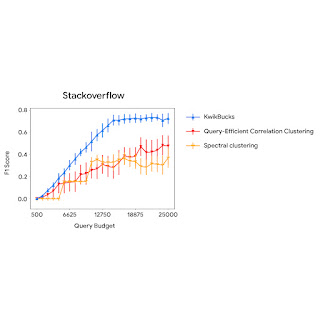
The figure below compares the clustering algorithm’s performance with baselines using different query budgets. We observe that KwikBucks consistently outperforms other baselines at various budgets.
 |
| A comparison of KwikBucks with top-2 baselines when allowed different budgets for querying the cross-attention model. |
Conclusion
Text clustering often presents a dilemma in the choice of similarity function: embedding models are scalable but lack quality, while cross-attention models offer quality but substantially hurt scalability. We present a clustering algorithm that offers the best of both worlds: the scalability of embedding models and the quality of cross-attention models. KwikBucks can also be applied to other clustering problems with multiple similarity oracles of varying accuracy levels. This is validated with an exhaustive set of experiments on various datasets with diverse properties. See the paper for more details.
Acknowledgements
This project was initiated during Sandeep Silwal’s summer internship at Google in 2022. We would like to express our gratitude to our co-authors, Andrew McCallum, Andrew Nystrom, Deepak Ramachandran, and Sandeep Silwal, for their valuable contributions to this work. We also thank Ravi Kumar and John Guilyard for assistance with this blog post.

‘Starship for the Mind’: University of Florida Opens Malachowsky Hall, an Epicenter for AI and Data Science
Embodying the convergence of AI and academia, the University of Florida Friday inaugurated the Malachowsky Hall for Data Science & Information Technology.
The sleek, seven-story building is poised to play a pivotal role in UF’s ongoing efforts to harness the transformative power of AI, reaffirming its stature as one of the nation’s leading public universities.
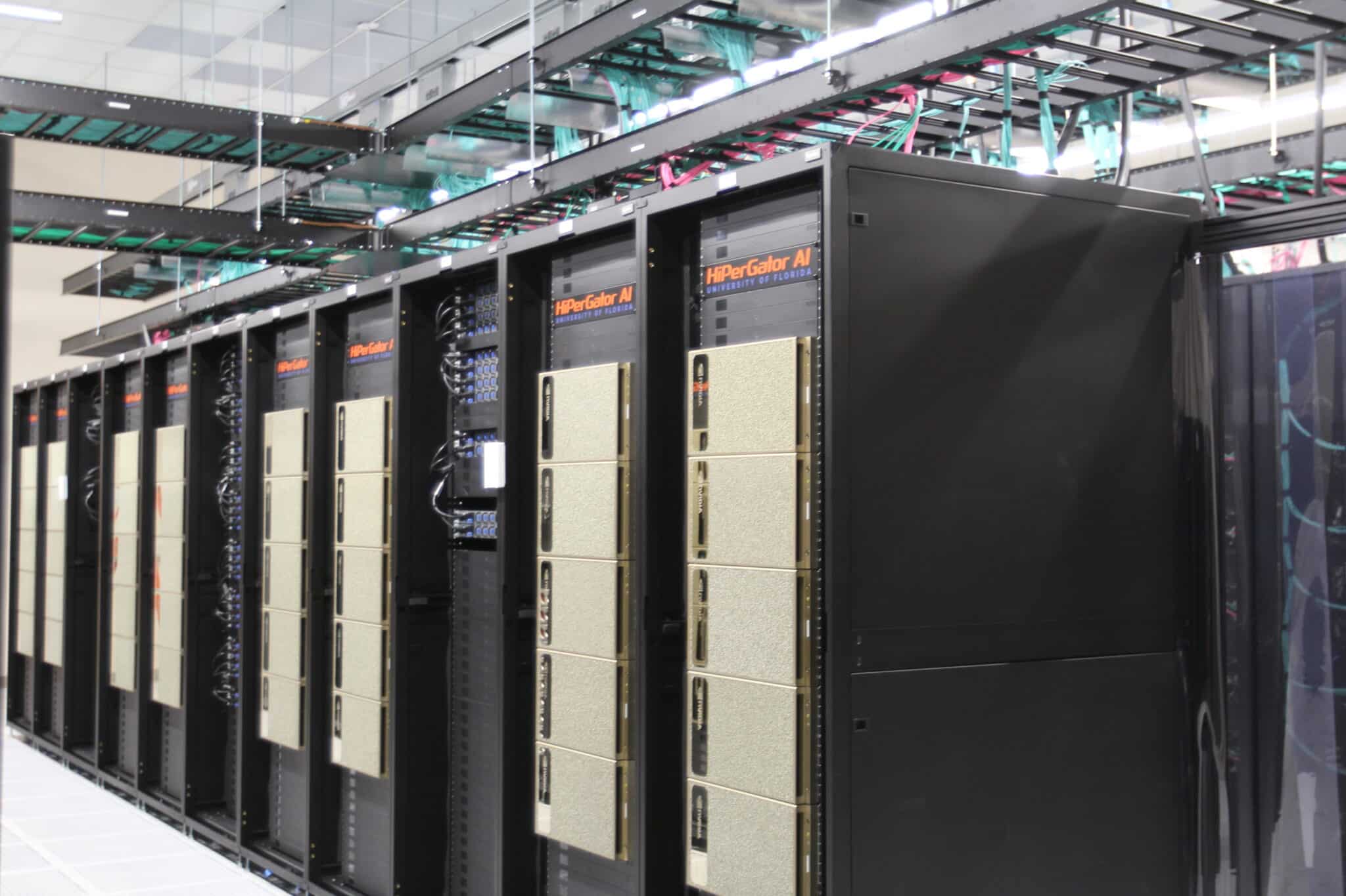
Evoking Apple co-founder Steve Jobs’ iconic description of a personal computer, NVIDIA’s founder and CEO Jensen Huang described Malachowsky Hall — named for NVIDIA co-founder Chris Malachowsky — and the HiPerGator AI supercomputer it hosts as a “starship for knowledge discovery.”
“Steve Jobs called (the PC) ‘the bicycle of the mind,’ a device that propels our thoughts further and faster,” Huang said.
“What Chris Malachowsky has gifted this institution is nothing short of the ‘starship of the mind’ — a vehicle that promises to take our intellect to uncharted territories,” Huang said.
The inauguration of the 260,000-square-foot structure marks a milestone in the partnership between UF alum Malachowsky, NVIDIA and the state of Florida — a collaboration that has propelled UF to the forefront of AI innovation.
Malachowsky and NVIDIA both made major contributions toward its construction, bolstered by a $110 million investment from the state of Florida.

Following the opening, Huang and UF’s new president, Ben Sasse, met to discuss the impact of AI and data science across UF and beyond for students just starting their careers.
Sasse underscored the importance of adaptability in a rapidly changing world, telling the audience: “work in lots and lots of different organizations … because lifelong work in any one, not just firm, but any one industry is going to end in our lives. You’re ultimately going to have to figure out how to reinvent yourselves at 30, 35, 40 and 45.”
Huang offered students very different advice, recalling how he met his wife, Lori, who was in the audience, as an undergraduate. “Have a good pickup line … do you want to know the pickup line?” Huang asked, pausing a beat. “You want to see my homework?”
The spirit of Sasse and Huang’s adaptable approach to career and personal development is embodied in Malachowsky Hall, designed to bring together people from academia and industry, research and government.
Packed with innovative collaboration spaces and labs, the hall features a spacious 400-seat auditorium, dedicated high-performance computing study spaces and a rooftop terrace that unveils panoramic campus vistas.
Sustainability is woven into its design, highlighted by energy-efficient systems and rainwater harvesting facilities.
Malachowsky Hall will serve as a conduit to bring the on-campus advances in AI to Florida’s thriving economy, which continues to outpace the nation in jobs and GDP growth.
UF’s efforts to bring AI and academia together, catalyzed by support from Malachowsky and NVIDIA, go far beyond Malachowsky Hall.
In 2020, UF announced that Malachowsky and NVIDIA together donated $50 million toward HiPerGator, one of the most powerful AI supercomputers in the country.
With additional state support, UF recently added more than 110 AI faculty members to the 300 already engaged in AI teaching and research.
As a result, UF extended AI-focused courses, workshops and projects across the university, enabling its 55,000 students to delve into AI and its interdisciplinary applications.
Friday’s ribbon-cutting will open exciting new opportunities for the university, its students and the state of Florida to realize the potential of AI innovations across sectors.
Huang likened pursuing knowledge through AI to embarking on a “starship.” “You’ve got to go as far as you can,” he urged students.
For a deeper exploration of Malachowsky Hall and UF’s groundbreaking AI initiatives, visit UF’s website.
Amazon and UIUC announce inaugural slate of funded research projects
Amazon-Illinois Center on Artificial Intelligence for Interactive Conversational Experiences also names first cohort of academic fellows.Read More

How AI-Based Cybersecurity Strengthens Business Resilience
The world’s 5 billion internet users and nearly 54 billion devices generate 3.4 petabytes of data per second, according to IDC. As digitalization accelerates, enterprise IT teams are under greater pressure to identify and block incoming cyber threats to ensure business operations and services are not interrupted — and AI-based cybersecurity provides a reliable way to do so.
Few industries appear immune to cyber threats. This year alone, international hotel chains, financial institutions, Fortune 100 retailers, air traffic-control systems and the U.S. government have all reported threats and intrusions.
Whether from insider error, cybercriminals, hacktivists or other threats, risks in the cyber landscape can damage an enterprise’s reputation and bottom line. A breach can paralyze operations, jeopardize proprietary and customer data, result in regulatory fines and destroy customer trust.
Using AI and accelerated computing, businesses can reduce the time and operational expenses required to detect and block cyber threats while freeing up resources to focus on core business value operations and revenue-generating activities.
Here’s a look at how industries are applying AI techniques to safeguard data, enable faster threat detection and mitigate attacks to ensure the consistent delivery of service to customers and partners.
Public Sector: Protecting Physical Security, Energy Security and Citizen Services
AI-powered analytics and automation tools are helping government agencies provide citizens with instant access to information and services, make data-driven decisions, model climate change, manage natural disasters, and more. But public entities managing digital tools and infrastructure face a complex cyber risk environment that includes regulatory compliance requirements, public scrutiny, large interconnected networks and the need to protect sensitive data and high-value targets.
Adversary nation-states may initiate cyberattacks to disrupt networks, steal intellectual property or swipe classified government documents. Internal misuse of digital tools and infrastructure combined with sophisticated external espionage places public organizations at high risk of data breach. Espionage actors have also been known to recruit inside help, with 16% of public administration breaches showing evidence of collusion. To protect critical infrastructure, citizen data, public records and other sensitive information, federal organizations are turning to AI.
The U.S. Department of Energy’s (DOE) Office of Cybersecurity, Energy Security and Emergency Response (CESER) is tasked with strengthening the resilience of the country’s energy sector by addressing emerging threats and improving energy infrastructure security. The DOE-CESER has invested more than $240 million in cybersecurity research, development and demonstration projects since 2010.
In one project, the department developed a tool that uses AI to automate and optimize security vulnerability and patch management in energy delivery systems. Another project for artificial diversity and defense security uses software-defined networks to enhance the situational awareness of energy delivery systems, helping ensure uninterrupted flows of energy.
The Defense Advanced Research Projects Agency (DARPA), which is charged with researching and investing in breakthrough technologies for national security, is using machine learning and AI in several areas. The DARPA CASTLE program trains AI to defend against advanced, persistent cyber threats. As part of the effort, researchers intend to accelerate cybersecurity assessments with approaches that are automated, repeatable and measurable. The DARPA GARD program builds platforms, libraries, datasets and training materials to help developers build AI models that are resistant to deception and adversarial attacks.
To keep up with an evolving threat landscape and ensure physical security, energy security and data security, public organizations must continue integrating AI to achieve a dynamic, proactive and far-reaching cyber defense posture.
Financial Services: Securing Digital Transactions, Payments and Portfolios
Banks, asset managers, insurers and other financial service organizations are using AI and machine learning to deliver superior performance in fraud detection, portfolio management, algorithmic trading and self-service banking.
With constant digital transactions, payments, loans and investment trades, financial service institutions manage some of the largest, most complex and most sensitive datasets of any industry. Behind only the healthcare industry, these organizations suffer the second highest cost of a data breach, at nearly $6 million per incident. This cost grows if regulators issue fines or if recovery includes legal fees and lawsuit settlements. Worse still, lost business may never be recovered if trust can’t be repaired.
Banks and financial institutions use AI to improve insider threat detection, detect phishing and ransomware, and keep sensitive information safe.
FinSec Innovation Lab, a joint venture by Mastercard and Enel X, is using AI to help its customers defend against ransomware. Prior to working with FinSec, one card-processing customer suffered a LockBit ransomware attack in which 200 company servers were infected in just 1.5 hours. The company was forced to shut down servers and suspend operations, resulting in an estimated $7 million in lost business.
FinSec replicated this attack in its lab but deployed the NVIDIA Morpheus cybersecurity framework, NVIDIA DOCA software framework for intrusion detection and NVIDIA BlueField DPU computing clusters. With this mix of AI and accelerated computing, FinSec was able to detect the ransomware attack in less than 12 seconds, quickly isolate virtual machines and recover 80% of the data on infected servers. This type of real-time response helps businesses avoid service downtime and lost business while maintaining customer trust.
With AI to help defend against cyberattacks, financial institutions can identify intrusions and anticipate future threats to keep financial records, accounts and transactions secure.
Retail: Keeping Sales Channels and Payment Credentials Safe
Retailers are using AI to power personalized product recommendations, dynamic pricing and customized marketing campaigns. Multichannel digital platforms have made in-store and online shopping more convenient: up to 48% of consumers save a card on file with a merchant, significantly boosting card-not-present transactions. While digitization has brought convenience, it has also made sensitive data more accessible to attackers.
Sitting on troves of digital payment credentials for millions of customers, retailers are a prime target for cybercriminals looking to take advantage of security gaps. According to a recent Data Breach Investigations Report from Verizon, 37% of confirmed data disclosures in the retail industry resulted in stolen payment card data.
Malware attacks, ransomware and distributed denial of service attacks are all on the rise, but phishing remains the favored vector for an initial attack. With a successful phishing intrusion, criminals can steal credentials, access systems and launch ransomware.
Best Buy manages a network of more than 1,000 stores across the U.S. and Canada. With multichannel digital sales across both countries, protecting consumer information and transactions is critical. To defend against phishing and other cyber threats, Best Buy began using customized machine learning and NVIDIA Morpheus to better secure their infrastructure and inform their security analysts.
After deploying this AI-based cyber defense, the retail giant improved the accuracy of phishing detection to 96% while reducing false-positive rates. With a proactive approach to cybersecurity, Best Buy is protecting its reputation as a tech expert focused on customer needs.
From complex supply chains to third-party vendors and multichannel point-of-sale networks, expect retailers to continue integrating AI to protect operations as well as critical proprietary and customer data.
Smart Cities and Spaces: Protecting Critical Infrastructure and Transit Networks
IoT devices and AI that analyze movement patterns, traffic and hazardous situations have great potential to improve the safety and efficiency of spaces and infrastructure. But as airports, shipping ports, transit networks and other smart spaces integrate IoT and use data, they also become more vulnerable to attack.
In the last couple of years, there have been distributed denial of service (DDoS) attacks on airports and air traffic control centers and ransomware attacks on seaports, city municipalities, police departments and more. Attacks can paralyze information systems, ground flights, disrupt the flow of cargo and traffic, and delay the delivery of goods to markets. Hostile attacks could have far more serious consequences, including physical harm or loss of life.
In connected spaces, AI-driven security can analyze vast amounts of data to predict threats, isolate attacks and provide rapid self-healing after an intrusion. AI algorithms trained on emails can halt threats in the inbox and block phishing attempts like those that delivered ransomware to seaports earlier this year. Machine learning can be trained to recognize DDoS attack patterns to prevent the type of incoming malicious traffic that brought down U.S. airport websites last year.
Organizations adopting smart space technology, such as the Port of Los Angeles, are making efforts to get ahead of the threat landscape. In 2014, the Port of LA established a cybersecurity operations center and hired a dedicated cybersecurity team. In 2021, the port followed up with a cyber resilience center to enhance early-warning detection for cyberattacks that have the potential to impact the flow of cargo.
The U.S. Federal Aviation Administration has developed an AI certification framework that assesses the trustworthiness of AI and ML applications. The FAA also implements a zero-trust cyber approach, enforces strict access control and runs continuous verification across its digital environment.
By bolstering cybersecurity and integrating AI, smart space and transport infrastructure administrators can offer secure access to physical spaces and digital networks to protect the uninterrupted movement of people and goods.
Telecommunications: Ensure Network Resilience and Block Incoming Threats
Telecommunications companies are leaning into AI to power predictive maintenance and maximum network uptime, network optimization, equipment troubleshooting, call-routing and self-service systems.
The industry is responsible for critical national infrastructure in every country, supports over 5 billion customer endpoints and is expected to constantly deliver above 99% reliability. As reliance on cloud, IoT and edge computing expands and 5G becomes the norm, immense digital surface areas must be protected from misuse and malicious attack.
Telcos can deploy AI to ensure the security and resilience of networks. AI can monitor IoT devices and edge networks to detect anomalies and intrusions, identify fake users, mitigate attacks and quarantine infected devices. AI can continuously assess the trustworthiness of devices, users and applications, thereby shortening the time needed to identify fraudsters.
Pretrained AI models can be deployed to protect 5G networks from threats such as malware, data exfiltration and DOS attacks.
Using deep learning and NVIDIA BlueField DPUs, Palo Alto Networks has built a next-generation firewall addressing 5G needs, maximizing cybersecurity performance while maintaining a small infrastructure footprint. The DPU powers accelerated intelligent network filtering to parse, classify and steer traffic to improve performance and isolate threats. With more efficient computing that deploys fewer servers, telcos can maximize return on investment for compute investments and minimize digital attack surface areas.
By putting AI to work, telcos can build secure, encrypted networks to ensure network availability and data security for both individual and enterprise customers.
Automotive: Insulate Vehicle Software From Outside Influence and Attack
Modern cars rely on complex AI and ML software stacks running on in-vehicle computers to process data from cameras and other sensors. These vehicles are essentially giant, moving IoT devices — they perceive the environment, make decisions, advise drivers and even control the vehicle with autonomous driving features.
Like other connected devices, autonomous vehicles are susceptible to various types of cyberattacks. Bad actors can infiltrate and compromise AV software both on board and from third-party providers. Denial of service attacks can disrupt over-the-air software updates that vehicles rely on to operate safely. Unauthorized access to communications systems like onboard WiFi, Bluetooth or RFID can expose vehicle systems to the risk of remote manipulation and data theft. This can jeopardize geolocation and sensor data, operational data, driver and passenger data, all of which are crucial to functional safety and the driving experience.
AI-based cybersecurity can help monitor in-car and network activities in real time, allowing for rapid response to threats. AI can be deployed to secure and authenticate over-the-air updates to prevent tampering and ensure the authenticity of software updates. AI-driven encryption can protect data transmitted over WiFi, Bluetooth and RFID connections. AI can also probe vehicle systems for vulnerabilities and take remedial steps.
Ranging from AI-powered access control to unlock and start vehicles to detecting deviations in sensor performance and patching security vulnerabilities, AI will play a crucial role in the safe development and deployment of autonomous vehicles on our roads.
Keeping Operations Secure and Customers Happy With AI Cybersecurity
By deploying AI to protect valuable data and digital operations, industries can focus their resources on innovating better products, improving customer experiences and creating new business value.
NVIDIA offers a number of tools and frameworks to help enterprises swiftly adjust to the evolving cyber risk environment. The NVIDIA Morpheus cybersecurity framework provides developers and software vendors with optimized, easy-to-use tools to build solutions that can proactively detect and mitigate threats while drastically reducing the cost of cyber defense operations. To help defend against phishing attempts, the NVIDIA spear phishing detection AI workflow uses NVIDIA Morpheus and synthetic training data created with the NVIDIA NeMo generative AI framework to flag and halt inbox threats.
The Morpheus SDK also enables digital fingerprinting to collect and analyze behavior characteristics for every user, service, account and machine across a network to identify atypical behavior and alert network operators. With the NVIDIA DOCA software framework, developers can create software-defined, DPU-accelerated services, while leveraging zero trust to build more secure applications.
AI-based cybersecurity empowers developers across industries to build solutions that can identify, capture and act on threats and anomalies to ensure business continuity and uninterrupted service, keeping operations safe and customers happy.
Learn how AI can help your organization achieve a proactive cybersecurity posture to protect customer and proprietary data to the highest standards.
Bundesliga Match Facts Shot Speed – Who fires the hardest shots in the Bundesliga?
There’s a kind of magic that surrounds a soccer shot so powerful, it leaves spectators, players, and even commentators in a momentary state of awe. Think back to a moment when the sheer force of a strike left an entire Bundesliga stadium buzzing with energy. What exactly captures our imagination with such intensity? While there are many factors that contribute to an iconic goal, there’s a particular magnetism to shots that blaze through the air, especially those taken from a distance.
Over the years, the Bundesliga has witnessed players who’ve become legends, not just for their skill but for their uncanny ability to unleash thunderbolts. Bernd Nickel, a standout figure from Frankfurt’s illustrious squad in the 1970s and 1980s, earned the title “Dr. Hammer” from ardent fans. Over his illustrious career, he netted 141 times in 426 matches.
Beyond his shooting prowess, another feat of Nickel’s that stands out is his ability to directly score from corner kicks. In fact, he holds the unique distinction of having scored from all four corner positions at Frankfurt’s Waldstadion. An example was witnessed by Frankfurt’s fans in May 1971, during a high-stakes game against Kickers Offenbach when he unveiled a masterclass.
Nickel scored a stunning goal in the 17th minute, which eventually led Frankfurt to a 2:0 victory. What made this goal even more memorable was the manner in which it was executed—a spectacular sideways scissors-kick from the penalty spot, fitting perfectly into the top corner. This goal would later be recognized as the “Goal of the Month” for May 1971. Nickl’s impact on the field was undeniable, and during the time he represented Eintracht Frankfurt, the club won the DFB-Pokal three times (in 1974, 1975, and 1981) and the UEFA Cup once in 1980.
Similarly, Thomas “the Hammer” Hitzlsberger has etched his name into Bundesliga folklore with his stunning left-footed rockets. His 2009 strike against Leverkusen at a speed of 125 km/h is one that is vividly remembered because the sheer velocity of Hitzlsperger’s free-kick was enough to leave Germany’s number one goalkeeper, René Adler, seemingly petrified.
Struck during the fifty-first minute of the game from a distance of 18 meters, the ball soared past Adler, leaving him motionless, and bulged the net, making the score 2:0. This remarkable goal not only showcased Hitzlsperger’s striking ability but also demonstrated the awe-inspiring power that such high-velocity goals can have on a match.
Historical data has shown us a few instances where the ball’s velocity exceeded the 130 km/h mark in Bundesliga, with the all-time record being a jaw-dropping shot at 137 km/h by Bayern’s Roy Makaay.
With all this in mind, it becomes even clearer why the speed and technique behind every shot matters immensely. Although high shooting speed excites soccer fans, it has not been measured regularly in the Bundesliga until now. Recognizing this, we are excited to introduce the new Bundesliga Match Facts: Shot Speed. This new metric aims to shed light on the velocity behind these incredible goals, enhancing our understanding and appreciation of the game even further.

How it works
Have you ever wondered just how fast a shot from your favorite Bundesliga player travels? The newly introduced Bundesliga Match Facts (BMF) Shot Speed now allows fans to satisfy their curiosity by providing insights into the incredible power and speed behind shots. Shot speed is more than just a number; it’s a window into the awe-inspiring athleticism and skill of the Bundesliga players.
Shot speed has a captivating effect on fans, igniting debates about which player possesses the most potent shot in the league and who consistently delivers lightning-fast strikes. Shot speed data is the key to resolving these questions.
Besides that, the new BMF helps to highlight memorable moments. The fastest shots often result in spectacular goals that live long in the memory of fans. Shot speed helps immortalize these moments, allowing fans to relive the magic of those lightning-fast strikes.
But how does this work? Let’s delve into the details.
Data collection process
A foundation of shot speed calculation lies in an organized data collection process. This process comprises two key components: event data and optical tracking data.
Event data collection entails gathering the fundamental building blocks of the game. Shots, goals, assists, fouls, and substitutions provide vital context for understanding what happens on the pitch. In our specific case, we focus on shots, their variations, and the players responsible for them.
On the flip side, optical tracking data is collected using advanced camera systems. These systems record player movements and ball positions, offering a high level of precision. This data serves as the bedrock for comprehensive analysis of player performance, tactical intricacies, and team strategies. When it comes to calculating shot speed, this data is essential for tracking the velocity of the ball.
These two streams of data originate from distinct sources, and their synchronization in time is not guaranteed. For the precision needed in shot speed calculations, we must ensure that the ball’s position aligns precisely with the moment of the event. This eliminates any discrepancies that might arise from the manual collection of event data. To achieve this, our process uses a synchronization algorithm that is trained on a labeled dataset. This algorithm robustly associates each shot with its corresponding tracking data.
Shot speed calculation
The heart of determining shot speed lies in a precise timestamp given by our synchronization algorithm. Imagine a player getting ready to take a shot. Our event gatherers are ready to record the moment, and cameras closely track the ball’s movement. The magic happens exactly when the player decides to pull the trigger.
An accurate timestamp measurement helps us figure out how fast the shot was right from the start. We measure shot speed for shots that end up as goals, those that hit the post, or get saved. To make sure we’re consistent, we don’t include headers or shots that get blocked. These can get a bit tricky due to deflections.
Let’s break down how we transform the collected data into the shot speed you see:
- Extracting shot trajectory – After recording the event and tracking the ball’s movement, we extract the trajectory of the shot. This means we map out the path the ball takes from the moment it leaves the player’s foot.
- Smoothing velocity curve – The data we get is detailed but can sometimes have tiny variations due to factors like camera sensitivity. To ensure accuracy, we smooth out the velocity curve. This means we remove any minor bumps or irregularities in the data to get a more reliable speed measurement.
- Calculating maximum speed – With a clean velocity curve in hand, we then calculate the maximum speed the ball reaches during its flight. This is the key number that represents the shot’s speed and power.
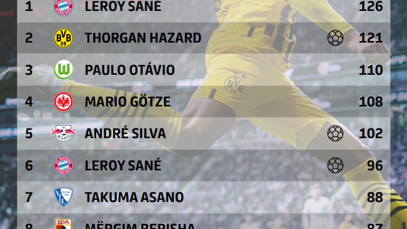
We analyzed around 215 matches from the Bundesliga 2022–2023 season. The following plot shows the number of fast shots (>100 km/h) by player. The 263 players with at least one fast shot (>100 km/h) have, on average, 3.47 fast shots. As the graph shows, some players have a frequency way above average, with around 20 fast shots.

Let’s look at some examples from the current season (2023–2024)
The following videos show examples of measured shots that achieved top-speed values.
Example 1
Measured with top shot speed 118.43 km/h with a distance to goal of 20.61 m
Example 2
Measured with top shot speed 123.32 km/h with a distance to goal of 21.19 m
Example 3
Measured with top shot speed 121.22 km/h with a distance to goal of 25.44 m
Example 4
Measured with top shot speed 113.14 km/h with a distance to goal of 24.46 m
How it’s implemented
In our quest to accurately determine shot speed during live matches, we’ve implemented a cutting-edge solution using Amazon Managed Streaming for Apache Kafka (Amazon MSK). This robust platform serves as the backbone for seamlessly streaming positional data at a rapid 25 Hz sampling rate, enabling real-time updates of shot speed. Through Amazon MSK, we’ve established a centralized hub for data streaming and messaging, facilitating seamless communication between containers for sharing a wealth of Bundesliga Match Facts.
The following diagram outlines the entire workflow for measuring shot speed from start to finish.
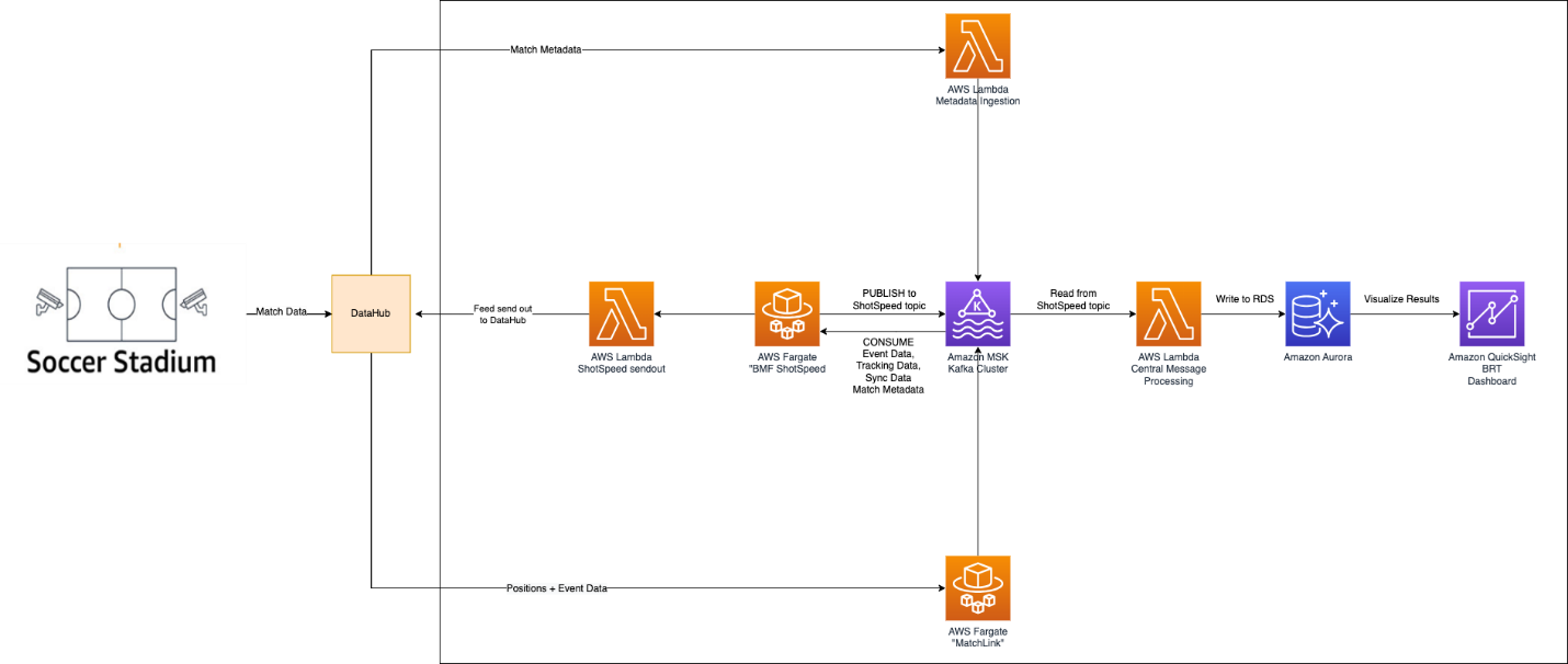
Match-related data is gathered and brought into the system via DFL’s DataHub. To process match metadata, we use an AWS Lambda function called MetaDataIngestion, while positional data is brought in using an AWS Fargate container known as MatchLink. These Lambda functions and Fargate containers then make this data available for further use in the appropriate MSK topics.
At the heart of the BMF Shot Speed lies a dedicated Fargate container named BMF ShotSpeed. This container is active throughout the duration of the match, continuously pulling in all the necessary data from Amazon MSK. Its algorithm responds instantly to every shot taken during the game, calculating the shot speed in real time. Moreover, we have the capability to recompute shot speed should any underlying data undergo updates.
Once the shot speeds have undergone their calculations, the next phase in our data journey is the distribution. The shot speed metrics are transmitted back to DataHub, where they are made available to various consumers of Bundesliga Match Facts.
Simultaneously, the shot speed data finds its way to a designated topic within our MSK cluster. This allows other components of Bundesliga Match Facts to access and take advantage of this metric. We’ve implemented an AWS Lambda function with the specific task of retrieving the calculated shot speed from the relevant Kafka topic. Once the Lambda function is triggered, it stores the data in an Amazon Aurora Serverless database. This database houses the shot speed data, which we then use to create interactive, near real-time visualizations using Amazon QuickSight.
Beyond this, we have a dedicated component specifically designed to calculate a seasonal ranking of shot speeds. This allows us to keep track of the fastest shots throughout the season, ensuring that we always have up-to-date information about the fastest shots and their respective rankings after each shot is taken.
Summary
In this blog post, we’re excited to introduce the all-new Bundesliga Match Facts: Shot Speed, a metric that allows us to quantify and objectively compare the velocity of shots taken by different Bundesliga players. This statistic will provide commentators and fans with valuable insights into the power and speed of shots on goal.
The development of the Bundesliga Match Facts is the result of extensive analysis conducted by a collaborative team of soccer experts and data scientists from the Bundesliga and AWS. Notable shot speeds will be displayed in real time on the live ticker during matches, accessible through the official Bundesliga app and website. Additionally, this data will be made readily available to commentators via the Data Story Finder and visually presented to fans at key moments during broadcasts.
We’re confident that the introduction of this brand-new Bundesliga Match Fact will enhance your understanding of the game and add a new dimension to your viewing experience. To delve deeper into the partnership between AWS and Bundesliga, please visit Bundesliga on AWS!
We’re eagerly looking forward to the insights you uncover with this new Shot Speed metric. Share your findings with us on X: @AWScloud, using the hashtag #BundesligaMatchFacts.

About the Authors
Tareq Haschemi is a consultant within AWS Professional Services. His skills and areas of expertise include application development, data science, and machine learning (ML). He supports customers in developing data-driven applications within the AWS Cloud. Prior to joining AWS, he was also a consultant in various industries, such as aviation and telecommunications. He is passionate about enabling customers on their data and artificial intelligence (AI) journey to the cloud.
Jean-Michel Lourier is a Senior Data Scientist within AWS Professional Services. He leads teams implementing data-driven applications side-by-side with AWS customers to generate business value out of their data. He’s passionate about diving into tech and learning about AI, ML, and their business applications. He is also an enthusiastic cyclist, taking long bike-packing trips.
Luc Eluère is a Data Scientist within Sportec Solutions AG. His mission is to develop and provide valuable KPIs to the soccer industry. At university, he learned the statistical theory with a goal: to apply its concepts to the beautiful game. Even though he was promised a nice career in table soccer, his passion for data science took over, and he chose computers as a career path.
Javier Poveda-Panter is a Senior Data and Machine Learning Engineer for EMEA sports customers within the AWS Professional Services team. He enables customers in the area of spectator sports to innovate and capitalize on their data, delivering high-quality user and fan experiences through ML, data science, and analytics. He follows his passion for a broad range of sports, music, and AI in his spare time.
Zero-shot adaptive prompting of large language models
Recent advances in large language models (LLMs) are very promising as reflected in their capability for general problem-solving in few-shot and zero-shot setups, even without explicit training on these tasks. This is impressive because in the few-shot setup, LLMs are presented with only a few question-answer demonstrations prior to being given a test question. Even more challenging is the zero-shot setup, where the LLM is directly prompted with the test question only.
Even though the few-shot setup has dramatically reduced the amount of data required to adapt a model for a specific use-case, there are still cases where generating sample prompts can be challenging. For example, handcrafting even a small number of demos for the broad range of tasks covered by general-purpose models can be difficult or, for unseen tasks, impossible. For example, for tasks like summarization of long articles or those that require domain knowledge (e.g., medical question answering), it can be challenging to generate sample answers. In such situations, models with high zero-shot performance are useful since no manual prompt generation is required. However, zero-shot performance is typically weaker as the LLM is not presented with guidance and thus is prone to spurious output.
In “Better Zero-shot Reasoning with Self-Adaptive Prompting”, published at ACL 2023, we propose Consistency-Based Self-Adaptive Prompting (COSP) to address this dilemma. COSP is a zero-shot automatic prompting method for reasoning problems that carefully selects and constructs pseudo-demonstrations for LLMs using only unlabeled samples (that are typically easy to obtain) and the models’ own predictions. With COSP, we largely close the performance gap between zero-shot and few-shot while retaining the desirable generality of zero-shot prompting. We follow this with “Universal Self-Adaptive Prompting“ (USP), accepted at EMNLP 2023, in which we extend the idea to a wide range of general natural language understanding (NLU) and natural language generation (NLG) tasks and demonstrate its effectiveness.
Prompting LLMs with their own outputs
Knowing that LLMs benefit from demonstrations and have at least some zero-shot abilities, we wondered whether the model’s zero-shot outputs could serve as demonstrations for the model to prompt itself. The challenge is that zero-shot solutions are imperfect, and we risk giving LLMs poor quality demonstrations, which could be worse than no demonstrations at all. Indeed, the figure below shows that adding a correct demonstration to a question can lead to a correct solution of the test question (Demo1 with question), whereas adding an incorrect demonstration (Demo 2 + questions, Demo 3 with questions) leads to incorrect answers. Therefore, we need to select reliable self-generated demonstrations.
 |
| Example inputs & outputs for reasoning tasks, which illustrates the need for carefully designed selection procedure for in-context demonstrations (MultiArith dataset & PaLM-62B model): (1) zero-shot chain-of-thought with no demo: correct logic but wrong answer; (2) correct demo (Demo1) and correct answer; (3) correct but repetitive demo (Demo2) leads to repetitive outputs; (4) erroneous demo (Demo3) leads to a wrong answer; but (5) combining Demo3 and Demo1 again leads to a correct answer. |
COSP leverages a key observation of LLMs: that confident and consistent predictions are more likely correct. This observation, of course, depends on how good the uncertainty estimate of the LLM is. Luckily, in large models, previous works suggest that the uncertainty estimates are robust. Since measuring confidence requires only model predictions, not labels, we propose to use this as a zero-shot proxy of correctness. The high-confidence outputs and their inputs are then used as pseudo-demonstrations.
With this as our starting premise, we estimate the model’s confidence in its output based on its self-consistency and use this measure to select robust self-generated demonstrations. We ask LLMs the same question multiple times with zero-shot chain-of-thought (CoT) prompting. To guide the model to generate a range of possible rationales and final answers, we include randomness controlled by a “temperature” hyperparameter. In an extreme case, if the model is 100% certain, it should output identical final answers each time. We then compute the entropy of the answers to gauge the uncertainty — the answers that have high self-consistency and for which the LLM is more certain, are likely to be correct and will be selected.
Assuming that we are presented with a collection of unlabeled questions, the COSP method is:
- Input each unlabeled question into an LLM, obtaining multiple rationales and answers by sampling the model multiple times. The most frequent answers are highlighted, followed by a score that measures consistency of answers across multiple sampled outputs (higher is better). In addition to favoring more consistent answers, we also penalize repetition within a response (i.e., with repeated words or phrases) and encourage diversity of selected demonstrations. We encode the preference towards consistent, un-repetitive and diverse outputs in the form of a scoring function that consists of a weighted sum of the three scores for selection of the self-generated pseudo-demonstrations.
- We concatenate the pseudo-demonstrations into test questions, feed them to the LLM, and obtain a final predicted answer.
 |
| Illustration of COSP: In Stage 1 (left), we run zero-shot CoT multiple times to generate a pool of demonstrations (each consisting of the question, generated rationale and prediction) and assign a score. In Stage 2 (right), we augment the current test question with pseudo-demos (blue boxes) and query the LLM again. A majority vote over outputs from both stages forms the final prediction. |
COSP focuses on question-answering tasks with CoT prompting for which it is easy to measure self-consistency since the questions have unique correct answers. But this can be difficult for other tasks, such as open-ended question-answering or generative tasks that don’t have unique answers (e.g., text summarization). To address this limitation, we introduce USP in which we generalize our approach to other general NLP tasks:
- Classification (CLS): Problems where we can compute the probability of each class using the neural network output logits of each class. In this way, we can measure the uncertainty without multiple sampling by computing the entropy of the logit distribution.
- Short-form generation (SFG): Problems like question answering where we can use the same procedure mentioned above for COSP, but, if necessary, without the rationale-generating step.
- Long-form generation (LFG): Problems like summarization and translation, where the questions are often open-ended and the outputs are unlikely to be identical, even if the LLM is certain. In this case, we use an overlap metric in which we compute the average of the pairwise ROUGE score between the different outputs to the same query.
 |
| Illustration of USP in exemplary tasks (classification, QA and text summarization). Similar to COSP, the LLM first generates predictions on an unlabeled dataset whose outputs are scored with logit entropy, consistency or alignment, depending on the task type, and pseudo-demonstrations are selected from these input-output pairs. In Stage 2, the test instances are augmented with pseudo-demos for prediction. |
We compute the relevant confidence scores depending on the type of task on the aforementioned set of unlabeled test samples. After scoring, similar to COSP, we pick the confident, diverse and less repetitive answers to form a model-generated pseudo-demonstration set. We finally query the LLM again in a few-shot format with these pseudo-demonstrations to obtain the final predictions on the entire test set.
Key Results
For COSP, we focus on a set of six arithmetic and commonsense reasoning problems, and we compare against 0-shot-CoT (i.e., “Let’s think step by step“ only). We use self-consistency in all baselines so that they use roughly the same amount of computational resources as COSP. Compared across three LLMs, we see that zero-shot COSP significantly outperforms the standard zero-shot baseline.
 |
| Key results of COSP in six arithmetic (MultiArith, GSM-8K, AddSub, SingleEq) and commonsense (CommonsenseQA, StrategyQA) reasoning tasks using PaLM-62B, PaLM-540B and GPT-3 (code-davinci-001) models. |
 |
| USP improves significantly on 0-shot performance. “CLS” is an average of 15 classification tasks; “SFG” is the average of five short-form generation tasks; “LFG” is the average of two summarization tasks. “SFG (BBH)” is an average of all BIG-Bench Hard tasks, where each question is in SFG format. |
For USP, we expand our analysis to a much wider range of tasks, including more than 25 classifications, short-form generation, and long-form generation tasks. Using the state-of-the-art PaLM 2 models, we also test against the BIG-Bench Hard suite of tasks where LLMs have previously underperformed compared to people. We show that in all cases, USP again outperforms the baselines and is competitive to prompting with golden examples.
 |
| Accuracy on BIG-Bench Hard tasks with PaLM 2-M (each line represents a task of the suite). The gain/loss of USP (green stars) over standard 0-shot (green triangles) is shown in percentages. “Human” refers to average human performance; “AutoCoT” and “Random demo” are baselines we compared against in the paper; and “3-shot” is the few-shot performance for three handcrafted demos in CoT format. |
We also analyze the working mechanism of USP by validating the key observation above on the relation between confidence and correctness, and we found that in an overwhelming majority of the cases, USP picks confident predictions that are more likely better in all task types considered, as shown in the figure below.
 |
| USP picks confident predictions that are more likely better. Ground-truth performance metrics against USP confidence scores in selected tasks in various task types (blue: CLS, orange: SFG, green: LFG) with PaLM-540B. |
Conclusion
Zero-shot inference is a highly sought-after capability of modern LLMs, yet the success in which poses unique challenges. We propose COSP and USP, a family of versatile, zero-shot automatic prompting techniques applicable to a wide range of tasks. We show large improvement over the state-of-the-art baselines over numerous task and model combinations.
Acknowledgements
This work was conducted by Xingchen Wan, Ruoxi Sun, Hootan Nakhost, Hanjun Dai, Julian Martin Eisenschlos, Sercan Ö. Arık, and Tomas Pfister. We would like to thank Jinsung Yoon Xuezhi Wang for providing helpful reviews, and other colleagues at Google Cloud AI Research for their discussion and feedback.
Using teacher knowledge at inference time to enhance student model
New method improves the state of the art in knowledge distillation by leveraging a knowledge base of teacher predictions.Read More
Deploy ML models built in Amazon SageMaker Canvas to Amazon SageMaker real-time endpoints
Amazon SageMaker Canvas now supports deploying machine learning (ML) models to real-time inferencing endpoints, allowing you take your ML models to production and drive action based on ML-powered insights. SageMaker Canvas is a no-code workspace that enables analysts and citizen data scientists to generate accurate ML predictions for their business needs.
Until now, SageMaker Canvas provided the ability to evaluate an ML model, generate bulk predictions, and run what-if analyses within its interactive workspace. But now you can also deploy the models to Amazon SageMaker endpoints for real-time inferencing, making it effortless to consume model predictions and drive actions outside the SageMaker Canvas workspace. Having the ability to directly deploy ML models from SageMaker Canvas eliminates the need to manually export, configure, test, and deploy ML models into production, thereby saving reducing complexity and saving time. It also makes operationalizing ML models more accessible to individuals, without the need to write code.
In this post, we walk you through the process to deploy a model in SageMaker Canvas to a real-time endpoint.
Overview of solution
For our use case, we are assuming the role of a business user in the marketing department of a mobile phone operator, and we have successfully created an ML model in SageMaker Canvas to identify customers with the potential risk of churn. Thanks to the predictions generated by our model, we now want to move this from our development environment to production. To streamline the process of deploying our model endpoint for inference, we directly deploy ML models from SageMaker Canvas, thereby eliminating the need to manually export, configure, test, and deploy ML models into production. This helps reduce complexity, saves time, and also makes operationalizing ML models more accessible to individuals, without the need to write code.
The workflow steps are as follows:
- Upload a new dataset with the current customer population into SageMaker Canvas. For the full list of supported data sources, refer to Import data into Canvas.
- Build ML models and analyze their performance metrics. For instructions, refer to Build a custom model and Evaluate Your Model’s Performance in Amazon SageMaker Canvas.
- Deploy the approved model version as an endpoint for real-time inferencing.
You can perform these steps in SageMaker Canvas without writing a single line of code.
Prerequisites
For this walkthrough, make sure that the following prerequisites are met:
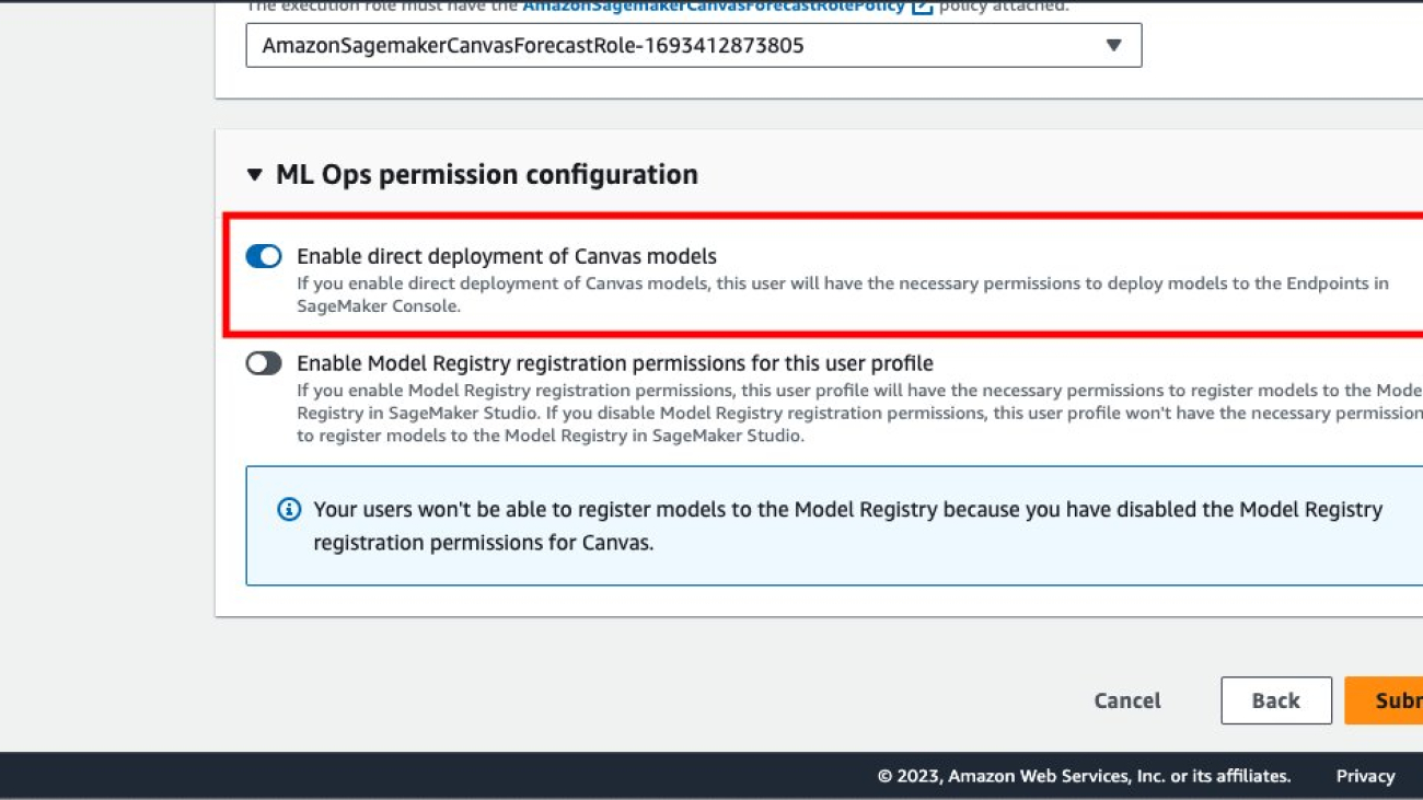
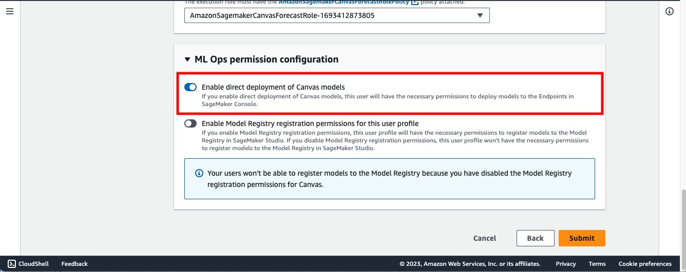
- To deploy model versions to SageMaker endpoints, the SageMaker Canvas admin must give the necessary permissions to the SageMaker Canvas user, which you can manage in the SageMaker domain that hosts your SageMaker Canvas application. For more information, refer to Permissions Management in Canvas.
- Implement the prerequisites mentioned in Predict customer churn with no-code machine learning using Amazon SageMaker Canvas.
You should now have three model versions trained on historical churn prediction data in Canvas:
- V1 trained with all 21 features and quick build configuration with a model score of 96.903%
- V2 trained with all 19 features (removed phone and state features) and quick build configuration and improved accuracy of 97.403%
- V3 trained with standard build configuration with 97.103% model score

Use the customer churn prediction model
Enable Show advanced metrics on the model details page and review the objective metrics associated with each model version so that you can select the best-performing model for deploying to SageMaker as an endpoint.

Based on the performance metrics, we select version 2 to be deployed.

Configure the model deployment settings—deployment name, instance type, and instance count.

As a starting point, Canvas will automatically recommend the best instance type and the number of instances for your model deployment. You can change it as per your workload needs.


You can test the deployed SageMaker inference endpoint directly from within SageMaker Canvas.

You can change input values using the SageMaker Canvas user interface to infer additional churn prediction.

Now let’s navigate to Amazon SageMaker Studio and check out the deployed endpoint.

Open a notebook in SageMaker Studio and run the following code to infer the deployed model endpoint. Replace the model endpoint name with your own model endpoint name.

Our original model endpoint is using an ml.m5.xlarge instance and 1 instance count. Now, let’s assume you expect the number of end-users inferencing your model endpoint will increase and you want to provision more compute capacity. You can accomplish this directly from within SageMaker Canvas by choosing Update configuration.


Clean up
To avoid incurring future charges, delete the resources you created while following this post. This includes logging out of SageMaker Canvas and deleting the deployed SageMaker endpoint. SageMaker Canvas bills you for the duration of the session, and we recommend logging out of SageMaker Canvas when you’re not using it. Refer to Logging out of Amazon SageMaker Canvas for more details.

Conclusion
In this post, we discussed how SageMaker Canvas can deploy ML models to real-time inferencing endpoints, allowing you take your ML models to production and drive action based on ML-powered insights. In our example, we showed how an analyst can quickly build a highly accurate predictive ML model without writing any code, deploy it on SageMaker as an endpoint, and test the model endpoint from SageMaker Canvas, as well as from a SageMaker Studio notebook.
To start your low-code/no-code ML journey, refer to Amazon SageMaker Canvas.
Special thanks to everyone who contributed to the launch: Prashanth Kurumaddali, Abishek Kumar, Allen Liu, Sean Lester, Richa Sundrani, and Alicia Qi.
About the Authors
 Janisha Anand is a Senior Product Manager in the Amazon SageMaker Low/No Code ML team, which includes SageMaker Canvas and SageMaker Autopilot. She enjoys coffee, staying active, and spending time with her family.
 Indy Sawhney is a Senior Customer Solutions Leader with Amazon Web Services. Always working backward from customer problems, Indy advises AWS enterprise customer executives through their unique cloud transformation journey. He has over 25 years of experience helping enterprise organizations adopt emerging technologies and business solutions. Indy is an area of depth specialist with AWS’s Technical Field Community for AI/ML, with specialization in generative AI and low-code/no-code Amazon SageMaker solutions.