 The Checks team shares three things that privacy professionals should consider when thinking about AI and privacy in 2024.Read More

The Checks team shares three things that privacy professionals should consider when thinking about AI and privacy in 2024.Read More

AI is reshaping industries, society and the “very fabric of innovation” — and Canada is poised to play a key role in this global transformation, said NVIDIA founder and CEO Jensen Huang during a fireside chat with leaders from across Canada’s thriving AI ecosystem.
“Canada, as you know, even though you’re so humble, you might not acknowledge it, is the epicenter of the invention of modern AI,” Huang told an audience of more than 400 from academia, industry and government gathered Thursday in Toronto.
In a pivotal development, Canada’s Industry Minister François-Philippe Champagne shared Friday on X, formerly known as Twitter, that Canada has signed a letter of intent with NVIDIA.
Nations including Canada, France, India and Japan are discussing the importance of investing in “sovereign AI capabilities,” Huang said in an interview with Bloomberg Television in Canada.
Such efforts promise to enhance domestic computing capabilities, turbocharging local economies and unlocking local talent.
“Their natural resource, data, should be refined and produced for their country. The recognition of sovereign AI capabilities is global,” Huang told Bloomberg.
Huang’s conversation with the group of Canadian AI leaders, or “four heroes of mine,” as he described them — Raquel Urtasun of Waabi, Brendan Frey of Deep Genomics, University of Toronto Professor Alan Aspuru-Guzik and Aiden Gomez of Cohere — highlighted both Canada’s enormous contributions and its growing capability as a leader in AI.
“Each one of you,” Huang remarked, addressing the panelists and noting that every one of them is affiliated with the University of Toronto, “are doing foundational work in some of the largest industries in the world.”
“Let’s seize the moment,” Champagne said as he kicked off the panel discussion. “We need to move from fear to opportunity to build trust so that people understand what AI can do for them.”
“It’s about inspiring young researchers to continue to do research here in Canada and about creating opportunities for them after they graduate to be able to start companies here,” Huang said.
The panelists echoed Huang’s optimism, providing insights into how AI is reshaping industries, society and technology.
Gomez, reflecting on the democratization of AI, shared his optimism for the future, stating that it’s “an exciting time to explore product space,” highlighting the vast opportunities for innovation and disruption within the AI landscape.
Cohere’s world-class large language models help enterprises build powerful, secure applications that search, understand meaning and converse in text.
Gomez said the future lies in communities of researchers and entrepreneurs able to leverage AI to bridge technological divides and foster inclusivity.
“I owe everything to this community, the people on the stage and in this room,” he said, acknowledging the collaborative spirit that fuels innovation in AI technologies.
Urtasun highlighted the imperative of safety in autonomous technology as a non-negotiable standard, emphasizing its role in saving lives and shaping the future of transportation.
“Safety should not be proprietary. This technology is a driver, and it’s going to save so many lives,” she said.
Frey underscored the transformative impact of AI in RNA biology. He said that, while “it’s taken quite a bit of time,” at Deep Genomics, he and his colleagues have built the world’s first foundation model for RNA biology, envisioning a future where drug discovery is accelerated, bringing life-saving therapies to market more efficiently.
“If we’re highly successful, best-case scenario, it means that we will be able to design molecules that are safe, and highly efficacious, without doing any cell model studies without doing any animal studies … and getting drugs that save our loved ones rapidly and safely,” Frey said.
Aspuru-Guzik pointed to the fusion of AI with quantum computing and materials science as a frontier for sustainable solutions, emphasizing the importance of creating a conducive environment for innovation in Canada.
“We want to build it here in Canada,” he said.
His work exemplifies the potential of AI to accelerate the development of new materials, driving forward a sustainable future.
Together, these visions articulate a future where AI enhances societal well-being, drives scientific advancement and fosters an inclusive, global community of innovation.
“AI is about the greatest opportunity to close the technology divide and be inclusive, for everybody to enjoy the technology revolution,” Huang said.
For more on the fast-growing impact of AI across the globe, visit NVIDIA’s AI nations hub.
Featured image credit: Christian Raul Hernandez, Creative Commons Attribution-Share Alike 4.0 International license.

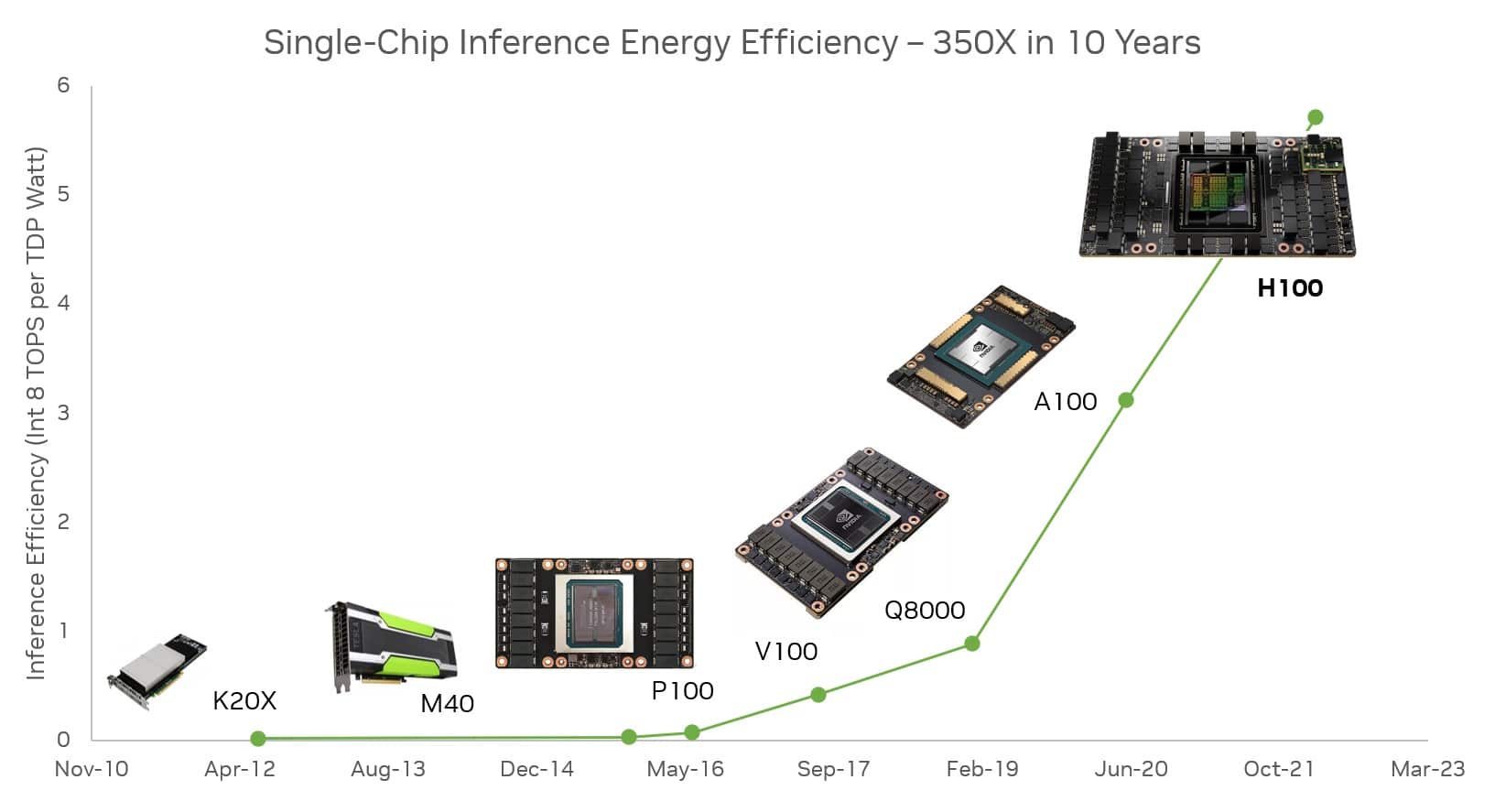
A new study underscores the potential of AI and accelerated computing to deliver energy efficiency and combat climate change, efforts in which NVIDIA has long been deeply engaged.
The study, called “Rethinking Concerns About AI’s Energy Use,” provides a well-researched examination into how AI can — and in many cases already does — play a large role in addressing these critical needs.
Citing dozens of sources, the study from the Information Technology and Innovation Foundation (ITIF), a Washington-based think tank focused on science and technology policy, calls for governments to accelerate adoption of AI as a significant new tool to drive energy efficiency across many industries.
AI can help “reduce carbon emissions, support clean energy technologies, and address climate change,” it said.
The report documents ways machine learning is already helping many sectors reduce their impact on the environment.
For example, it noted:
In these and many other ways, the study argues that AI advances energy efficiency. So, it calls on policymakers “to ensure AI is part of the solution, not part of the problem, when it comes to the environment.”
It also recommends adopting AI broadly across government agencies to “help the public sector reduce carbon emissions through more efficient digital services, smart cities and buildings, intelligent transportation systems, and other AI-enabled efficiencies.”
The study’s author, Daniel Castro, saw in current predictions about AI a repeat of exaggerated forecasts that emerged during the rise of the internet more than two decades ago.
“People extrapolate from early studies, but don’t consider all the important variables including improvements you see over time in digitalization like energy efficiency,” said Castro, who leads ITIF’s Center for Data Innovation.
“The danger is policymakers could miss the big picture and hold back beneficial uses of AI that are having positive impacts, especially in regulated areas like healthcare,” he said.
“For example, we’ve had electronic health records since the 1980s, but it took focused government investments to get them deployed,” he added. “Now AI brings big opportunities for decarbonization across the government and the economy.”
Data centers of every size have a part to play in maximizing their energy efficiency with AI and accelerated computing.
For instance, NVIDIA’s AI-based weather-prediction model, FourCastNet, is about 45,000x faster and consumes 12,000x less energy to produce a forecast than current techniques. That promises efficiency boosts for supercomputers around the world that run continuously to provide regional forecasts, Bjorn Stevens, director of the Max Planck Institute for Meteorology, said in a blog.
Overall, data centers could save a whopping 19 terawatt-hours of electricity a year if all AI, high performance computing and networking offloads were run on GPU and DPU accelerators instead of CPUs, according to NVIDIA’s calculations. That’s the equivalent of the energy consumption of 2.9 million passenger cars driven for a year.
Last year, the U.S. Department of Energy’s lead facility for open science documented its advances with accelerated computing.
Using NVIDIA A100 Tensor Core GPUs, energy efficiency improved 5x on average across four key scientific applications in tests at the National Energy Research Scientific Computing Center. An application for weather forecasting logged gains of nearly 10x.
The combination of accelerated computing and AI is creating new scientific instruments to help understand and combat climate change.
In 2021, NVIDIA announced Earth-2, an initiative to build a digital twin of Earth on a supercomputer capable of simulating climate on a global scale. It’s among a handful of similarly ambitious efforts around the world.
An example is Destination Earth, a pan-European project to create digital twins of the planet, that’s using accelerated computing, AI and “collaboration on an unprecedented scale,” said the project’s leader, Peter Bauer, a veteran with more than 20 years at Europe’s top weather-forecasting center.
Experts in the utility sector agree AI is key to advancing sustainability.
“AI will play a crucial role maintaining stability for an electric grid that’s becoming exponentially more complex with large numbers of low-capacity, variable generation sources like wind and solar coming online, and two-way power flowing into and out of houses,” said Jeremy Renshaw, a senior program manager at the Electric Power Research Institute, an independent nonprofit that collaborates with more than 450 companies in 45 countries, in a blog.
Learn more about sustainable computing as well as NVIDIA’s commitment to use 100% renewable energy starting in fiscal year 2025. And watch the video below for more on how AI is accelerating efforts to combat climate change.
A look at our collaboration with humanitarian organizations to use flood forecasting technology.Read More


Time-series forecasting is ubiquitous in various domains, such as retail, finance, manufacturing, healthcare and natural sciences. In retail use cases, for example, it has been observed that improving demand forecasting accuracy can meaningfully reduce inventory costs and increase revenue. Deep learning (DL) models have emerged as a popular approach for forecasting rich, multivariate, time-series data because they have proven to perform well in a variety of settings (e.g., DL models dominated the M5 competition leaderboard).
At the same time, there has been rapid progress in large foundation language models used for natural language processing (NLP) tasks, such as translation, retrieval-augmented generation, and code completion. These models are trained on massive amounts of textual data derived from a variety of sources like common crawl and open-source code that allows them to identify patterns in languages. This makes them very powerful zero-shot tools; for instance, when paired with retrieval, they can answer questions about and summarize current events.
Despite DL-based forecasters largely outperforming traditional methods and progress being made in reducing training and inference costs, they face challenges: most DL architectures require long and involved training and validation cycles before a customer can test the model on a new time-series. A foundation model for time-series forecasting, in contrast, can provide decent out-of-the-box forecasts on unseen time-series data with no additional training, enabling users to focus on refining forecasts for the actual downstream task like retail demand planning.
To that end, in “A decoder-only foundation model for time-series forecasting”, we introduce TimesFM, a single forecasting model pre-trained on a large time-series corpus of 100 billion real world time-points. Compared to the latest large language models (LLMs), TimesFM is much smaller (200M parameters), yet we show that even at such scales, its zero-shot performance on a variety of unseen datasets of different domains and temporal granularities come close to the state-of-the-art supervised approaches trained explicitly on these datasets. Later this year we plan to make this model available for external customers in Google Cloud Vertex AI.
LLMs are usually trained in a decoder-only fashion that involves three steps. First, text is broken down into subwords called tokens. Then, the tokens are fed into stacked causal transformer layers that produce an output corresponding to each input token (it cannot attend to future tokens). Finally, the output corresponding to the i-th token summarizes all the information from previous tokens and predicts the (i+1)-th token. During inference, the LLM generates the output one token at a time. For example, when prompted with “What is the capital of France?”, it might generate the token “The”, then condition on “What is the capital of France? The” to generate the next token “capital” and so on until it generates the complete answer: “The capital of France is Paris”.
A foundation model for time-series forecasting should adapt to variable context (what we observe) and horizon (what we query the model to forecast) lengths, while having enough capacity to encode all patterns from a large pretraining dataset. Similar to LLMs, we use stacked transformer layers (self-attention and feedforward layers) as the main building blocks for the TimesFM model. In the context of time-series forecasting, we treat a patch (a group of contiguous time-points) as a token that was popularized by a recent long-horizon forecasting work. The task then is to forecast the (i+1)-th patch of time-points given the i-th output at the end of the stacked transformer layers.
However, there are several key differences from language models. Firstly, we need a multilayer perceptron block with residual connections to convert a patch of time-series into a token that can be input to the transformer layers along with positional encodings (PE). For that, we use a residual block similar to our prior work in long-horizon forecasting. Secondly, at the other end, an output token from the stacked transformer can be used to predict a longer length of subsequent time-points than the input patch length, i.e., the output patch length can be larger than the input patch length.
Consider a time-series of length 512 time-points being used to train a TimesFM model with input patch length 32 and output patch length 128. During training, the model is simultaneously trained to use the first 32 time-points to forecast the next 128 time-points, the first 64 time-points to forecast time-points 65 to 192, the first 96 time-points to forecast time-points 97 to 224 and so on. During inference, suppose the model is given a new time-series of length 256 and tasked with forecasting the next 256 time-points into the future. The model will first generate the future predictions for time-points 257 to 384, then condition on the initial 256 length input plus the generated output to generate time-points 385 to 512. On the other hand, if in our model the output patch length was equal to the input patch length of 32 then for the same task we would have to go through eight generation steps instead of just the two above. This increases the chances of more errors accumulating and therefore, in practice, we see that a longer output patch length yields better performance for long-horizon forecasting
 |
| TimesFM architecture. |
Just like LLMs get better with more tokens, TimesFM requires a large volume of legitimate time series data to learn and improve. We have spent a great amount of time creating and assessing our training datasets, and the following is what we have found works best:
Synthetic data helps with the basics. Meaningful synthetic time-series data can be generated using statistical models or physical simulations. These basic temporal patterns can teach the model the grammar of time series forecasting.
Real-world data adds real-world flavor. We comb through available public time series datasets, and selectively put together a large corpus of 100 billion time-points. Among these datasets there are Google Trends and Wikipedia Pageviews, which track what people are interested in, and that nicely mirrors trends and patterns in many other real-world time series. This helps TimesFM understand the bigger picture and generalize better when provided with domain-specific contexts not seen during training.
We evaluate TimesFM zero-shot on data not seen during training using popular time-series benchmarks. We observe that TimesFM performs better than most statistical methods like ARIMA, ETS and can match or outperform powerful DL models like DeepAR, PatchTST that have been explicitly trained on the target time-series.
We used the Monash Forecasting Archive to evaluate TimesFM’s out-of-the-box performance. This archive contains tens of thousands of time-series from various domains like traffic, weather, and demand forecasting covering frequencies ranging from few minutes to yearly data. Following existing literature, we inspect the mean absolute error (MAE) appropriately scaled so that it can be averaged across the datasets. We see that zero-shot (ZS) TimesFM is better than most supervised approaches, including recent deep learning models. We also compare TimesFM to GPT-3.5 for forecasting using a specific prompting technique proposed by llmtime(ZS). We demonstrate that TimesFM performs better than llmtime(ZS) despite being orders of magnitude smaller.
 |
| Scaled MAE (the lower the better) of TimesFM(ZS) against other supervised and zero-shot approaches on Monash datasets. |
Most of the Monash datasets are short or medium horizon, i.e., the prediction length is not too long. We also test TimesFM on popular benchmarks for long horizon forecasting against a recent state-of-the-art baseline PatchTST (and other long-horizon forecasting baselines). In the next figure, we plot the MAE on ETT datasets for the task of predicting 96 and 192 time-points into the future. The metric has been calculated on the last test window of each dataset (as done by the llmtime paper). We see that TimesFM not only surpasses the performance of llmtime(ZS) but also matches that of the supervised PatchTST model explicitly trained on the respective datasets.
 |
| Last window MAE (the lower the better) of TimesFM(ZS) against llmtime(ZS) and long-horizon forecasting baselines on ETT datasets. |
We train a decoder-only foundation model for time-series forecasting using a large pretraining corpus of 100B real world time-points, the majority of which was search interest time-series data derived from Google Trends and pageviews from Wikipedia. We show that even a relatively small 200M parameter pretrained model that uses our TimesFM architecture displays impressive zero-shot performance on a variety of public benchmarks from different domains and granularities.
This work is the result of a collaboration between several individuals across Google Research and Google Cloud, including (in alphabetical order): Abhimanyu Das, Weihao Kong, Andrew Leach, Mike Lawrence, Alex Martin, Rajat Sen, Yang Yang and Yichen Zhou.
![]() Google’s Super Bowl ad shows how Pixel’s Guided Frame helps blind or low vision people take great pictures or selfies.Read More
Google’s Super Bowl ad shows how Pixel’s Guided Frame helps blind or low vision people take great pictures or selfies.Read More


Machine learning models in the real world are often trained on limited data that may contain unintended statistical biases. For example, in the CELEBA celebrity image dataset, a disproportionate number of female celebrities have blond hair, leading to classifiers incorrectly predicting “blond” as the hair color for most female faces — here, gender is a spurious feature for predicting hair color. Such unfair biases could have significant consequences in critical applications such as medical diagnosis.
Surprisingly, recent work has also discovered an inherent tendency of deep networks to amplify such statistical biases, through the so-called simplicity bias of deep learning. This bias is the tendency of deep networks to identify weakly predictive features early in the training, and continue to anchor on these features, failing to identify more complex and potentially more accurate features.
With the above in mind, we propose simple and effective fixes to this dual challenge of spurious features and simplicity bias by applying early readouts and feature forgetting. First, in “Using Early Readouts to Mediate Featural Bias in Distillation”, we show that making predictions from early layers of a deep network (referred to as “early readouts”) can automatically signal issues with the quality of the learned representations. In particular, these predictions are more often wrong, and more confidently wrong, when the network is relying on spurious features. We use this erroneous confidence to improve outcomes in model distillation, a setting where a larger “teacher” model guides the training of a smaller “student” model. Then in “Overcoming Simplicity Bias in Deep Networks using a Feature Sieve”, we intervene directly on these indicator signals by making the network “forget” the problematic features and consequently look for better, more predictive features. This substantially improves the model’s ability to generalize to unseen domains compared to previous approaches. Our AI Principles and our Responsible AI practices guide how we research and develop these advanced applications and help us address the challenges posed by statistical biases.
 |
| Animation comparing hypothetical responses from two models trained with and without the feature sieve. |
We first illustrate the diagnostic value of early readouts and their application in debiased distillation, i.e., making sure that the student model inherits the teacher model’s resilience to feature bias through distillation. We start with a standard distillation framework where the student is trained with a mixture of label matching (minimizing the cross-entropy loss between student outputs and the ground-truth labels) and teacher matching (minimizing the KL divergence loss between student and teacher outputs for any given input).
Suppose one trains a linear decoder, i.e., a small auxiliary neural network named as Aux, on top of an intermediate representation of the student model. We refer to the output of this linear decoder as an early readout of the network representation. Our finding is that early readouts make more errors on instances that contain spurious features, and further, the confidence on those errors is higher than the confidence associated with other errors. This suggests that confidence on errors from early readouts is a fairly strong, automated indicator of the model’s dependence on potentially spurious features.
 |
| Illustrating the usage of early readouts (i.e., output from the auxiliary layer) in debiasing distillation. Instances that are confidently mispredicted in the early readouts are upweighted in the distillation loss. |
We used this signal to modulate the contribution of the teacher in the distillation loss on a per-instance basis, and found significant improvements in the trained student model as a result.
We evaluated our approach on standard benchmark datasets known to contain spurious correlations (Waterbirds, CelebA, CivilComments, MNLI). Each of these datasets contain groupings of data that share an attribute potentially correlated with the label in a spurious manner. As an example, the CelebA dataset mentioned above includes groups such as {blond male, blond female, non-blond male, non-blond female}, with models typically performing the worst on the {non-blond female} group when predicting hair color. Thus, a measure of model performance is its worst group accuracy, i.e., the lowest accuracy among all known groups present in the dataset. We improved the worst group accuracy of student models on all datasets; moreover, we also improved overall accuracy in three of the four datasets, showing that our improvement on any one group does not come at the expense of accuracy on other groups. More details are available in our paper.
 |
| Comparison of Worst Group Accuracies of different distillation techniques relative to that of the Teacher model. Our method outperforms other methods on all datasets. |
In a second, closely related project, we intervene directly on the information provided by early readouts, to improve feature learning and generalization. The workflow alternates between identifying problematic features and erasing identified features from the network. Our primary hypothesis is that early features are more prone to simplicity bias, and that by erasing (“sieving”) these features, we allow richer feature representations to be learned.
 |
| Training workflow with feature sieve. We alternate between identifying problematic features (using training iteration) and erasing them from the network (using forgetting iteration). |
We describe the identification and erasure steps in more detail:
We can control specifically how the feature sieve is applied to a given dataset through a small number of configuration parameters. By changing the position and complexity of the auxiliary network, we control the complexity of the identified- and erased features. By modifying the mixing of learning and forgetting steps, we control the degree to which the model is challenged to learn more complex features. These choices, which are dataset-dependent, are made via hyperparameter search to maximize validation accuracy, a standard measure of generalization. Since we include “no-forgetting” (i.e., the baseline model) in the search space, we expect to find settings that are at least as good as the baseline.
Below we show features learned by the baseline model (middle row) and our model (bottom row) on two benchmark datasets — biased activity recognition (BAR) and animal categorization (NICO). Feature importance was estimated using post-hoc gradient-based importance scoring (GRAD-CAM), with the orange-red end of the spectrum indicating high importance, while green-blue indicates low importance. Shown below, our trained models focus on the primary object of interest, whereas the baseline model tends to focus on background features that are simpler and spuriously correlated with the label.
 |
| Feature importance scoring using GRAD-CAM on activity recognition (BAR) and animal categorization (NICO) generalization benchmarks. Our approach (last row) focuses on the relevant objects in the image, whereas the baseline (ERM; middle row) relies on background features that are spuriously correlated with the label. |
Through this ability to learn better, generalizable features, we show substantial gains over a range of relevant baselines on real-world spurious feature benchmark datasets: BAR, CelebA Hair, NICO and ImagenetA, by margins up to 11% (see figure below). More details are available in our paper.
 |
| Our feature sieve method improves accuracy by significant margins relative to the nearest baseline for a range of feature generalization benchmark datasets. |
We hope that our work on early readouts and their use in feature sieving for generalization will both spur the development of a new class of adversarial feature learning approaches and help improve the generalization capability and robustness of deep learning systems.
The work on applying early readouts to debiasing distillation was conducted in collaboration with our academic partners Durga Sivasubramanian, Anmol Reddy and Prof. Ganesh Ramakrishnan at IIT Bombay. We extend our sincere gratitude to Praneeth Netrapalli and Anshul Nasery for their feedback and recommendations. We are also grateful to Nishant Jain, Shreyas Havaldar, Rachit Bansal, Kartikeya Badola, Amandeep Kaur and the whole cohort of pre-doctoral researchers at Google Research India for taking part in research discussions. Special thanks to Tom Small for creating the animation used in this post.
One of the most useful application patterns for generative AI workloads is Retrieval Augmented Generation (RAG). In the RAG pattern, we find pieces of reference content related to an input prompt by performing similarity searches on embeddings. Embeddings capture the information content in bodies of text, allowing natural language processing (NLP) models to work with language in a numeric form. Embeddings are just vectors of floating point numbers, so we can analyze them to help answer three important questions: Is our reference data changing over time? Are the questions users are asking changing over time? And finally, how well is our reference data covering the questions being asked?
In this post, you’ll learn about some of the considerations for embedding vector analysis and detecting signals of embedding drift. Because embeddings are an important source of data for NLP models in general and generative AI solutions in particular, we need a way to measure whether our embeddings are changing over time (drifting). In this post, you’ll see an example of performing drift detection on embedding vectors using a clustering technique with large language models (LLMS) deployed from Amazon SageMaker JumpStart. You’ll also be able to explore these concepts through two provided examples, including an end-to-end sample application or, optionally, a subset of the application.
The RAG pattern lets you retrieve knowledge from external sources, such as PDF documents, wiki articles, or call transcripts, and then use that knowledge to augment the instruction prompt sent to the LLM. This allows the LLM to reference more relevant information when generating a response. For example, if you ask an LLM how to make chocolate chip cookies, it can include information from your own recipe library. In this pattern, the recipe text is converted into embedding vectors using an embedding model, and stored in a vector database. Incoming questions are converted to embeddings, and then the vector database runs a similarity search to find related content. The question and the reference data then go into the prompt for the LLM.
Let’s take a closer look at the embedding vectors that get created and how to perform drift analysis on those vectors.
Embedding vectors are numeric representations of our data so analysis of these vectors can provide insight into our reference data that can later be used to detect potential signals of drift. Embedding vectors represent an item in n-dimensional space, where n is often large. For example, the GPT-J 6B model, used in this post, creates vectors of size 4096. To measure drift, assume that our application captures embedding vectors for both reference data and incoming prompts.
We start by performing dimension reduction using Principal Component Analysis (PCA). PCA tries to reduce the number of dimensions while preserving most of the variance in the data. In this case, we try to find the number of dimensions that preserves 95% of the variance, which should capture anything within two standard deviations.
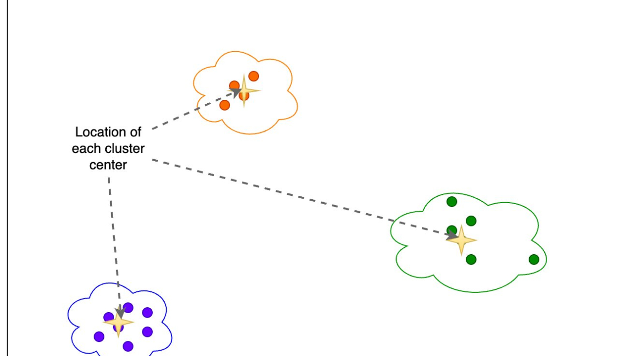
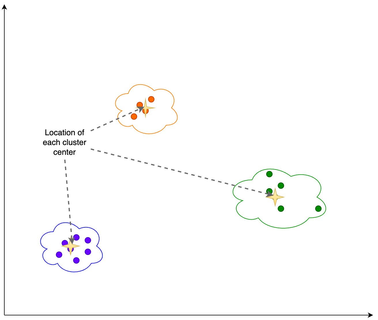
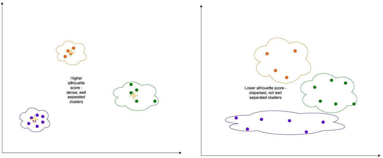
Then we use K-Means to identify a set of cluster centers. K-Means tries to group points together into clusters such that each cluster is relatively compact and the clusters are as distant from each other as possible.
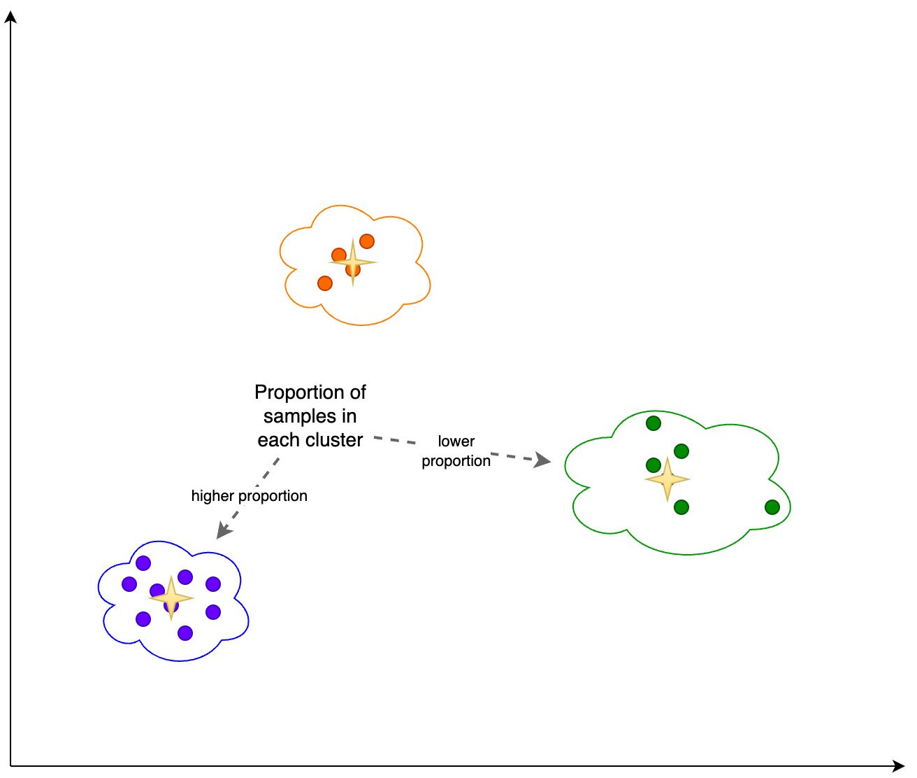
We calculate the following information based on the clustering output shown in the following figure:
Additionally, we look at the proportion (higher or lower) of samples in each cluster, as shown in the following figure.
Finally, we use this analysis to calculate the following:
We can periodically capture this information for snapshots of the embeddings for both the source reference data and the prompts. Capturing this data allows us to analyze potential signals of embedding drift.
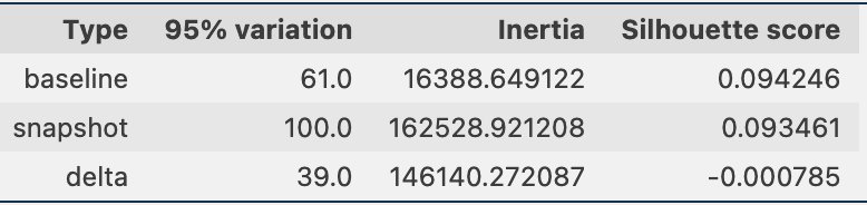
Periodically, we can compare the clustering information through snapshots of the data, which includes the reference data embeddings and the prompt embeddings. First, we can compare the number of dimensions needed to explain 95% of the variation in the embedding data, the inertia, and the silhouette score from the clustering job. As you can see in the following table, compared to a baseline, the latest snapshot of embeddings requires 39 more dimensions to explain the variance, indicating that our data is more dispersed. The inertia has gone up, indicating that the samples are in aggregate farther away from their cluster centers. Additionally, the silhouette score has gone down, indicating that the clusters are not as well defined. For prompt data, that might indicate that the types of questions coming into the system are covering more topics.
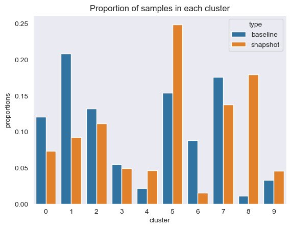
Next, in the following figure, we can see how the proportion of samples in each cluster has changed over time. This can show us whether our newer reference data is broadly similar to the previous set, or covers new areas.
Finally, we can see if the cluster centers are moving, which would show drift in the information in the clusters, as shown in the following table.
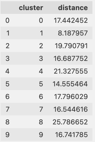
We can also evaluate how well our reference data aligns to the incoming questions. To do this, we assign each prompt embedding to a reference data cluster. We compute the distance from each prompt to its corresponding center, and look at the mean, median, and standard deviation of those distances. We can store that information and see how it changes over time.
The following figure shows an example of analyzing the distance between the prompt embedding and reference data centers over time.
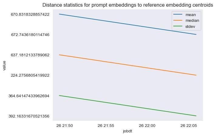
As you can see, the mean, median, and standard deviation distance statistics between prompt embeddings and reference data centers is decreasing between the initial baseline and the latest snapshot. Although the absolute value of the distance is difficult to interpret, we can use the trends to determine if the semantic overlap between reference data and incoming questions is getting better or worse over time.
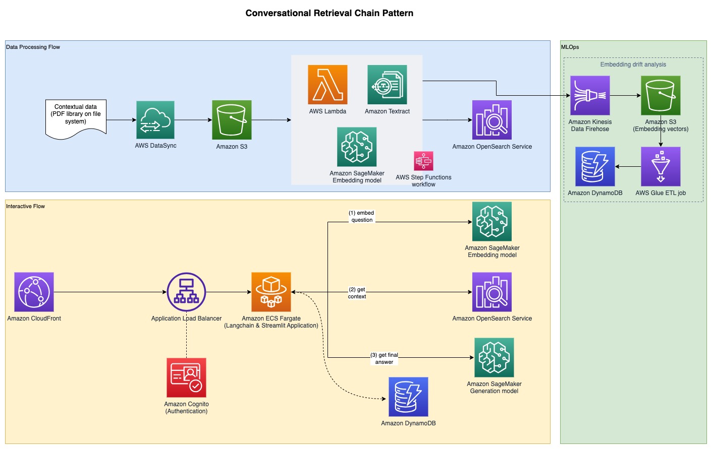
In order to gather the experimental results discussed in the previous section, we built a sample application that implements the RAG pattern using embedding and generation models deployed through SageMaker JumpStart and hosted on Amazon SageMaker real-time endpoints.
The application has three core components:
The following diagram illustrates the end-to-end architecture.
The full sample code is available on GitHub. The provided code is available in two different patterns:
To create the provided patterns, there are several prerequisites detailed in the following sections, starting with deploying the generative and text embedding models then moving on to the additional prerequisites.
Both patterns assume the deployment of an embedding model and generative model. For this, you’ll deploy two models from SageMaker JumpStart. The first model, GPT-J 6B, is used as the embedding model and the second model, Falcon-40b, is used for text generation.
You can deploy each of these models through SageMaker JumpStart from the AWS Management Console, Amazon SageMaker Studio, or programmatically. For more information, refer to How to use JumpStart foundation models. To simplify the deployment, you can use the provided notebook derived from notebooks automatically created by SageMaker JumpStart. This notebook pulls the models from the SageMaker JumpStart ML hub and deploys them to two separate SageMaker real-time endpoints.
The sample notebook also has a cleanup section. Don’t run that section yet, because it will delete the endpoints just deployed. You will complete the cleanup at the end of the walkthrough.
After confirming successful deployment of the endpoints, you’re ready to deploy the full sample application. However, if you’re more interested in exploring only the backend and analysis notebooks, you can optionally deploy only that, which is covered in the next section.
This pattern allows you to deploy the backend solution only and interact with the solution using a Jupyter notebook. Use this pattern if you don’t want to build out the full frontend interface.
You should have the following prerequisites:
Use the deployment parameters noted in the previous section to deploy the AWS CDK stack. For more information about AWS CDK installation, refer to Getting started with the AWS CDK.
Make sure that Docker is installed and running on the workstation that will be used for AWS CDK deployment. Refer to Get Docker for additional guidance.
Alternatively, you can enter the context values in a file called cdk.context.json in the pattern1-rag/cdk directory and run cdk deploy BackendStack --exclusively.
The deployment will print out outputs, some of which will be needed to run the notebook. Before you can start question and answering, embed the reference documents, as shown in the next section.
For this RAG approach, reference documents are first embedded with a text embedding model and stored in a vector database. In this solution, an ingestion pipeline has been built that intakes PDF documents.
An Amazon Elastic Compute Cloud (Amazon EC2) instance has been created for the PDF document ingestion and an Amazon Elastic File System (Amazon EFS) file system is mounted on the EC2 instance to save the PDF documents. An AWS DataSync task is run every hour to fetch PDF documents found in the EFS file system path and upload them to an S3 bucket to start the text embedding process. This process embeds the reference documents and saves the embeddings in OpenSearch Service. It also saves an embedding archive to an S3 bucket through Kinesis Data Firehose for later analysis.
To ingest the reference documents, complete the following steps:
JumpHostId) and connect using Session Manager, a capability of AWS Systems Manager. For instructions, refer to Connect to your Linux instance with AWS Systems Manager Session Manager./mnt/efs/fs1, which is where the EFS file system is mounted, and create a folder called ingest:
ingest directory.The DataSync task is configured to upload all files found in this directory to Amazon S3 to start the embedding process.
The DataSync task runs on an hourly schedule; you can optionally start the task manually to start the embedding process immediately for the PDF documents you added.
DataSyncTaskID and start the task with defaults.After the embeddings are created, you can start the RAG question and answering through a Jupyter notebook, as shown in the next section.
Complete the following steps:
NotebookInstanceName and connect to JupyterLab from the SageMaker console.fmops/full-stack/pattern1-rag/notebooks/.query-llm.ipynb in the notebook instance to perform question and answering using RAG.Make sure to use the conda_python3 kernel for the notebook.
This pattern is useful to explore the backend solution without needing to provision additional prerequisites that are required for the full-stack application. The next section covers the implementation of a full-stack application, including both the frontend and backend components, to provide a user interface for interacting with your generative AI application.
This pattern allows you to deploy the solution with a user frontend interface for question and answering.
To deploy the sample application, you must have the following prerequisites:
example.com.example.com and *.example.com for all subdomains. For instructions, refer to Requesting a public certificate. This certificate is used to configure HTTPS on Amazon CloudFront and the origin load balancer.app.example.com. app-lb.example.com.ZXXXXXXXXYYYYYYYYY.example.com.Use the deployment parameters you noted in the prerequisites to deploy the AWS CDK stack. For more information, refer to Getting started with the AWS CDK.
Make sure Docker is installed and running on the workstation that will be used for the AWS CDK deployment.
In the preceding code, -c represents a context value, in the form of the required prerequisites, provided on input. Alternatively, you can enter the context values in a file called cdk.context.json in the pattern1-rag/cdk directory and run cdk deploy --all.
Note that we specify the Region in the file bin/cdk.ts. Configuring ALB access logs requires a specified Region. You can change this Region before deployment.
The deployment will print out the URL to access the Streamlit application. Before you can start question and answering, you need to embed the reference documents, as shown in the next section.
For a RAG approach, reference documents are first embedded with a text embedding model and stored in a vector database. In this solution, an ingestion pipeline has been built that intakes PDF documents.
As we discussed in the first deployment option, an example EC2 instance has been created for the PDF document ingestion and an EFS file system is mounted on the EC2 instance to save the PDF documents. A DataSync task is run every hour to fetch PDF documents found in the EFS file system path and upload them to an S3 bucket to start the text embedding process. This process embeds the reference documents and saves the embeddings in OpenSearch Service. It also saves an embedding archive to an S3 bucket through Kinesis Data Firehose for later analysis.
To ingest the reference documents, complete the following steps:
JumpHostId) and connect using Session Manager./mnt/efs/fs1, which is where the EFS file system is mounted, and create a folder called ingest:
ingest directory.The DataSync task is configured to upload all files found in this directory to Amazon S3 to start the embedding process.
The DataSync task runs on an hourly schedule. You can optionally start the task manually to start the embedding process immediately for the PDF documents you added.
DataSyncTaskID and start the task with defaults.After the reference documents have been embedded, you can start the RAG question and answering by visiting the URL to access the Streamlit application. An Amazon Cognito authentication layer is used, so it requires creating a user account in the Amazon Cognito user pool deployed via the AWS CDK (see the AWS CDK output for the user pool name) for first-time access to the application. For instructions on creating an Amazon Cognito user, refer to Creating a new user in the AWS Management Console.
In this section, we show you how to perform drift analysis by first creating a baseline of the reference data embeddings and prompt embeddings, and then creating a snapshot of the embeddings over time. This allows you to compare the baseline embeddings to the snapshot embeddings.
To create an embedding baseline of the reference data, open the AWS Glue console and select the ETL job embedding-drift-analysis. Set the parameters for the ETL job as follows and run the job:
--job_type to BASELINE.--out_table to the Amazon DynamoDB table for reference embedding data. (See the AWS CDK output DriftTableReference for the table name.)--centroid_table to the DynamoDB table for reference centroid data. (See the AWS CDK output CentroidTableReference for the table name.)--data_path to the S3 bucket with the prefix; for example, s3://<REPLACE_WITH_BUCKET_NAME>/embeddingarchive/. (See the AWS CDK output BucketName for the bucket name.)Similarly, using the ETL job embedding-drift-analysis, create an embedding baseline of the prompts. Set the parameters for the ETL job as follows and run the job:
--job_type to BASELINE --out_table to the DynamoDB table for prompt embedding data. (See the AWS CDK output DriftTablePromptsName for the table name.)--centroid_table to the DynamoDB table for prompt centroid data. (See the AWS CDK output CentroidTablePrompts for the table name.) --data_path to the S3 bucket with the prefix; for example, s3://<REPLACE_WITH_BUCKET_NAME>/promptarchive/. (See the AWS CDK output BucketName for the bucket name.)After you ingest additional information into OpenSearch Service, run the ETL job embedding-drift-analysis again to snapshot the reference data embeddings. The parameters will be the same as the ETL job that you ran to create the embedding baseline of the reference data as shown in the previous section, with the exception of setting the --job_type parameter to SNAPSHOT.
Similarly, to snapshot the prompt embeddings, run the ETL job embedding-drift-analysis again. The parameters will be the same as the ETL job that you ran to create the embedding baseline for the prompts as shown in the previous section, with the exception of setting the --job_type parameter to SNAPSHOT.
To compare the embedding baseline and snapshot for reference data and prompts, use the provided notebook pattern1-rag/notebooks/drift-analysis.ipynb.
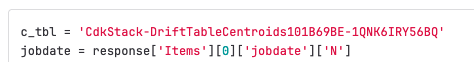
To look at embedding comparison for reference data or prompts, change the DynamoDB table name variables (tbl and c_tbl) in the notebook to the appropriate DynamoDB table for each run of the notebook.
The notebook variable tbl should be changed to the appropriate drift table name. The following is an example of where to configure the variable in the notebook.
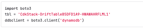
The table names can be retrieved as follows:
DriftTableReferenceDriftTablePromptsNameIn addition, the notebook variable c_tbl should be changed to the appropriate centroid table name. The following is an example of where to configure the variable in the notebook.
The table names can be retrieved as follows:
CentroidTableReferenceCentroidTablePromptsFirst, run the AWS Glue job embedding-distance-analysis. This job will find out which cluster, from the K-Means evaluation of the reference data embeddings, that each prompt belongs to. It then calculates the mean, median, and standard deviation of the distance from each prompt to the center of the corresponding cluster.
You can run the notebook pattern1-rag/notebooks/distance-analysis.ipynb to see the trends in the distance metrics over time. This will give you a sense of the overall trend in the distribution of the prompt embedding distances.
The notebook pattern1-rag/notebooks/prompt-distance-outliers.ipynb is an AWS Glue notebook that looks for outliers, which can help you identify whether you’re getting more prompts that are not related to the reference data.
All similarity scores from OpenSearch Service are logged in Amazon CloudWatch under the rag namespace. The dashboard RAG_Scores shows the average score and the total number of scores ingested.
To avoid incurring future charges, delete all the resources that you created.
Reference the cleanup up section of the provided example notebook to delete the deployed SageMaker JumpStart models, or you can delete the models on the SageMaker console.
If you entered your parameters in a cdk.context.json file, clean up as follows:
If you entered your parameters on the command line and only deployed the backend application (the backend AWS CDK stack), clean up as follows:
If you entered your parameters on the command line and deployed the full solution (the frontend and backend AWS CDK stacks), clean up as follows:
In this post, we provided a working example of an application that captures embedding vectors for both reference data and prompts in the RAG pattern for generative AI. We showed how to perform clustering analysis to determine whether reference or prompt data is drifting over time, and how well the reference data covers the types of questions users are asking. If you detect drift, it can provide a signal that the environment has changed and your model is getting new inputs that it may not be optimized to handle. This allows for proactive evaluation of the current model against changing inputs.
 Abdullahi Olaoye is a Senior Solutions Architect at Amazon Web Services (AWS). Abdullahi holds a MSC in Computer Networking from Wichita State University and is a published author that has held roles across various technology domains such as DevOps, infrastructure modernization and AI. He is currently focused on Generative AI and plays a key role in assisting enterprises to architect and build cutting-edge solutions powered by Generative AI. Beyond the realm of technology, he finds joy in the art of exploration. When not crafting AI solutions, he enjoys traveling with his family to explore new places.
 Randy DeFauw is a Senior Principal Solutions Architect at AWS. He holds an MSEE from the University of Michigan, where he worked on computer vision for autonomous vehicles. He also holds an MBA from Colorado State University. Randy has held a variety of positions in the technology space, ranging from software engineering to product management. In entered the Big Data space in 2013 and continues to explore that area. He is actively working on projects in the ML space and has presented at numerous conferences including Strata and GlueCon.
 Shelbee Eigenbrode is a Principal AI and Machine Learning Specialist Solutions Architect at Amazon Web Services (AWS). She has been in technology for 24 years spanning multiple industries, technologies, and roles. She is currently focusing on combining her DevOps and ML background into the domain of MLOps to help customers deliver and manage ML workloads at scale. With over 35 patents granted across various technology domains, she has a passion for continuous innovation and using data to drive business outcomes. Shelbee is a co-creator and instructor of the Practical Data Science specialization on Coursera. She is also the Co-Director of Women In Big Data (WiBD), Denver chapter. In her spare time, she likes to spend time with her family, friends, and overactive dogs.
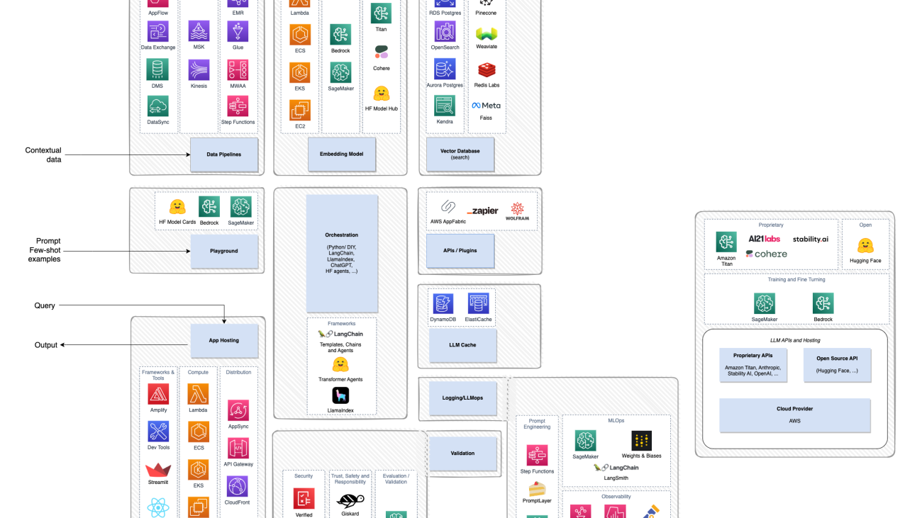
Resilience plays a pivotal role in the development of any workload, and generative AI workloads are no different. There are unique considerations when engineering generative AI workloads through a resilience lens. Understanding and prioritizing resilience is crucial for generative AI workloads to meet organizational availability and business continuity requirements. In this post, we discuss the different stacks of a generative AI workload and what those considerations should be.
Although a lot of the excitement around generative AI focuses on the models, a complete solution involves people, skills, and tools from several domains. Consider the following picture, which is an AWS view of the a16z emerging application stack for large language models (LLMs).

Compared to a more traditional solution built around AI and machine learning (ML), a generative AI solution now involves the following:
Unlike traditional AI models, Retrieval Augmented Generation (RAG) allows for more accurate and contextually relevant responses by integrating external knowledge sources. The following are some considerations when using RAG:
In cases where you need to provide contextual data to the foundation model using the RAG pattern, you need a data pipeline that can ingest the source data, convert it to embedding vectors, and store the embedding vectors in a vector database. This pipeline could be a batch pipeline if you prepare contextual data in advance, or a low-latency pipeline if you’re incorporating new contextual data on the fly. In the batch case, there are a couple challenges compared to typical data pipelines.
The data sources may be PDF documents on a file system, data from a software as a service (SaaS) system like a CRM tool, or data from an existing wiki or knowledge base. Ingesting from these sources is different from the typical data sources like log data in an Amazon Simple Storage Service (Amazon S3) bucket or structured data from a relational database. The level of parallelism you can achieve may be limited by the source system, so you need to account for throttling and use backoff techniques. Some of the source systems may be brittle, so you need to build in error handling and retry logic.
The embedding model could be a performance bottleneck, regardless of whether you run it locally in the pipeline or call an external model. Embedding models are foundation models that run on GPUs and do not have unlimited capacity. If the model runs locally, you need to assign work based on GPU capacity. If the model runs externally, you need to make sure you’re not saturating the external model. In either case, the level of parallelism you can achieve will be dictated by the embedding model rather than how much CPU and RAM you have available in the batch processing system.
In the low-latency case, you need to account for the time it takes to generate the embedding vectors. The calling application should invoke the pipeline asynchronously.
A vector database has two functions: store embedding vectors, and run a similarity search to find the closest k matches to a new vector. There are three general types of vector databases:
We don’t cover the similarity searching capabilities in detail in this post. Although they’re important, they are a functional aspect of the system and don’t directly affect resilience. Instead, we focus on the resilience aspects of a vector database as a storage system:
There are three unique considerations for the application tier when integrating generative AI solutions:
We can think about capacity in two contexts: inference and training model data pipelines. Capacity is a consideration when organizations are building their own pipelines. CPU and memory requirements are two of the biggest requirements when choosing instances to run your workloads.
Instances that can support generative AI workloads can be more difficult to obtain than your average general-purpose instance type. Instance flexibility can help with capacity and capacity planning. Depending on what AWS Region you are running your workload in, different instance types are available.
For the user journeys that are critical, organizations will want to consider either reserving or pre-provisioning instance types to ensure availability when needed. This pattern achieves a statically stable architecture, which is a resiliency best practice. To learn more about static stability in the AWS Well-Architected Framework reliability pillar, refer to Use static stability to prevent bimodal behavior.
Besides the resource metrics you typically collect, like CPU and RAM utilization, you need to closely monitor GPU utilization if you host a model on Amazon SageMaker or Amazon Elastic Compute Cloud (Amazon EC2). GPU utilization can change unexpectedly if the base model or the input data changes, and running out of GPU memory can put the system into an unstable state.
Higher up the stack, you will also want to trace the flow of calls through the system, capturing the interactions between agents and tools. Because the interface between agents and tools is less formally defined than an API contract, you should monitor these traces not only for performance but also to capture new error scenarios. To monitor the model or agent for any security risks and threats, you can use tools like Amazon GuardDuty.
You should also capture baselines of embedding vectors, prompts, context, and output, and the interactions between these. If these change over time, it may indicate that users are using the system in new ways, that the reference data is not covering the question space in the same way, or that the model’s output is suddenly different.
Having a business continuity plan with a disaster recovery strategy is a must for any workload. Generative AI workloads are no different. Understanding the failure modes that are applicable to your workload will help guide your strategy. If you are using AWS managed services for your workload, such as Amazon Bedrock and SageMaker, make sure the service is available in your recovery AWS Region. As of this writing, these AWS services don’t support replication of data across AWS Regions natively, so you need to think about your data management strategies for disaster recovery, and you also may need to fine-tune in multiple AWS Regions.
This post described how to take resilience into account when building generative AI solutions. Although generative AI applications have some interesting nuances, the existing resilience patterns and best practices still apply. It’s just a matter of evaluating each part of a generative AI application and applying the relevant best practices.
For more information about generative AI and using it with AWS services, refer to the following resources:
 Jennifer Moran is an AWS Senior Resiliency Specialist Solutions Architect based out of New York City. She has a diverse background, having worked in many technical disciplines, including software development, agile leadership, and DevOps, and is an advocate for women in tech. She enjoys helping customers design resilient solutions to improve resilience posture and publicly speaks about all topics related to resilience.
 Randy DeFauw is a Senior Principal Solutions Architect at AWS. He holds an MSEE from the University of Michigan, where he worked on computer vision for autonomous vehicles. He also holds an MBA from Colorado State University. Randy has held a variety of positions in the technology space, ranging from software engineering to product management. He entered the big data space in 2013 and continues to explore that area. He is actively working on projects in the ML space and has presented at numerous conferences, including Strata and GlueCon.
Data is the foundation to capturing the maximum value from AI technology and solving business problems quickly. To unlock the potential of generative AI technologies, however, there’s a key prerequisite: your data needs to be appropriately prepared. In this post, we describe how use generative AI to update and scale your data pipeline using Amazon SageMaker Canvas for data prep.
Typically, data pipeline work requires a specialized skill to prepare and organize data for security analysts to use to extract value, which can take time, increase risks, and increase time to value. With SageMaker Canvas, security analysts can effortlessly and securely access leading foundation models to prepare their data faster and remediate cyber security risks.
Data prep involves careful formatting and thoughtful contextualization, working backward from the customer problem. Now with the SageMaker Canvas chat for data prep capability, analysts with domain knowledge can quickly prepare, organize, and extract value from data using a chat-based experience.
Generative AI is revolutionizing the security domain by providing personalized and natural language experiences, enhancing risk identification and remediations, while boosting business productivity. For this use case, we use SageMaker Canvas, Amazon SageMaker Data Wrangler, Amazon Security Lake, and Amazon Simple Storage Service (Amazon S3). Amazon Security Lake allows you to aggregate and normalize security data for analysis to gain a better understanding of security across your organization. Amazon S3 enables you to store and retrieve any amount of data at any time or place. It offers industry-leading scalability, data availability, security, and performance.
SageMaker Canvas now supports comprehensive data preparation capabilities powered by SageMaker Data Wrangler. With this integration, SageMaker Canvas provides an end-to-end no-code workspace to prepare data, build, and use machine learning (ML) and Amazon Bedrock foundation models to accelerate the time from data to business insights. You can now discover and aggregate data from over 50 data sources and explore and prepare data using over 300 built-in analyses and transformations in the SageMaker Canvas visual interface. You’ll also see faster performance for transforms and analyses, and benefit from a natural language interface to explore and transform data for ML.
In this post, we demonstrate three key transformations; filtering, column renaming, and text extraction from a column on the security findings dataset. We also demonstrate using the chat for data prep feature in SageMaker Canvas to analyze the data and visualize your findings.
Before starting, you need an AWS account. You also need to set up an Amazon SageMaker Studio domain. For instructions on setting up SageMaker Canvas, refer to Generate machine learning predictions without code.
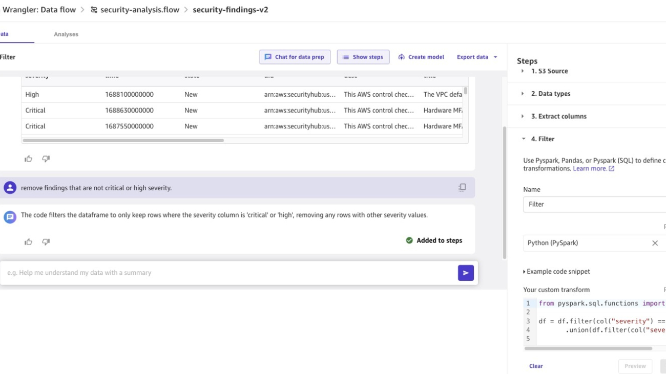
Complete the following steps to start using the SageMaker Canvas chat feature:
For this post, we first want to filter for critical and high severity warnings, so we enter into the chat box instructions to remove findings that are not critical or high severity. Canvas removes the rows, displays a preview of transformed data, and provides the option to use the code. We can add it to the list of steps in the Steps pane.

Next, we want rename two columns, so we enter in the chat box the following prompt, to rename the desc and title columns to Finding and Remediation. SageMaker Canvas generates a preview, and if you’re happy with the results, you can add the transformed data to the data flow steps.

To determine the source Regions of the findings, you can enter in chat instructions to Extract the Region text from the UID column based on the pattern arn:aws:security:securityhub:region:* and create a new column called Region) to extract the Region text from the UID column based on a pattern. SageMaker Canvas then generates code to create a new region column. The data preview shows the findings originate from one Region: us-west-2. You can add this transformation to the data flow for downstream analysis.

Finally, we want to analyze the data to determine if there is a correlation between time of day and number of critical findings. You can enter a request to summarize critical findings by time of day into the chat, and SageMaker Canvas returns insights that are useful for your investigation and analysis.

Next, we visualize the findings by severity over time to include in a leadership report. You can ask SageMaker Canvas to generate a bar chart of severity compared to time of day. In seconds, SageMaker Canvas has created the chart grouped by severity. You can add this visualization to the analysis in the data flow and download it for your report. The data shows the findings originate from one Region and happen at specific times. This gives us confidence on where to focus our security findings investigation to determine root causes and corrective actions.

To avoid incurring unintended charges, complete the following steps to clean up your resources:
In this post, we showed you how to use SageMaker Canvas as an end-to-end no-code workspace for data preparation to build and use Amazon Bedrock foundation models to accelerate time to gather business insights from data.
Note that this approach is not limited to security findings; you can apply this to any generative AI use case that uses data preparation at its core.
The future belongs to businesses that can effectively harness the power of generative AI and large language models. But to do so, we must first develop a solid data strategy and understand the art of data preparation. By using generative AI to structure our data intelligently, and working backward from the customer, we can solve business problems faster. With SageMaker Canvas chat for data preparation, it’s effortless for analysts to get started and capture immediate value from AI.
 Sudeesh Sasidharan is a Senior Solutions Architect at AWS, within the Energy team. Sudeesh loves experimenting with new technologies and building innovative solutions that solve complex business challenges. When he is not designing solutions or tinkering with the latest technologies, you can find him on the tennis court working on his backhand.
 John Klacynski is a Principal Customer Solution Manager within the AWS Independent Software Vendor (ISV) team. In this role, he programmatically helps ISV customers adopt AWS technologies and services to reach their business goals more quickly. Prior to joining AWS, John led Data Product Teams for large Consumer Package Goods companies, helping them leverage data insights to improve their operations and decision making.