When do recommender systems amplify user preferences? A theoretical framework and mitigation strategies

What the research is:

Recommender systems have come to influence nearly every aspect of human activity on the internet, whether in the news we read, the products we purchase, or the entertainment we consume. The algorithms and models at the heart of these systems rely on learning our preferences through the course of our interactions with them; when we watch a video or like a post on Facebook, we provide hints to the system about our preferences.

This repeated interplay between people and algorithms creates a feedback loop that results in recommendations that are increasingly customized to our tastes. Ideally, these feedback loops ought to be virtuous all the time; the recommender system is able to infer exactly what our preferences are and provides us with recommendations that enhance the quality of our lives.

However, what happens when the system overindexes and amplifies interactions that do not necessarily capture the user’s true preferences? Or if the user’s preferences have drifted toward recommended items that could be considered harmful or detrimental to their long-term well-being? Under what conditions would recommender systems respond to these changes and amplify preferences leading to a higher prevalence of harmful recommendations?

How it works:

In this paper, we provide a theoretical framework to answer these questions. We model the interactions between users and recommender systems and explore how these interactions may lead to potential harmful outcomes. Our main assumption is that users have a slight inclination to reinforce their opinion (or drift), i.e., increase their preference toward recommendations that they seem to correlate well with, and decrease it otherwise. We characterize the temporal evolution of the user’s preferences as a function of the user, the recommender system, and time, and ask whether this function admits a fixed point, i.e., any change in the system’s response to the user’s interactions does not change their preferences. We show that even under a mild drift and absent any external intervention, no such fixed point exists. That is, even a slight preference by a user for recommendations in a given category can lead to increasingly higher concentrations of item recommendations from that category. We refer to this phenomenon as preference amplification.

Recommender system model

We leverage the well-adopted collaborative filtering model of recommendation systems – each (user, item) tuple receives a score based on the likelihood of the user to be interested in the item. These scores are computed using low-dimension matrix factorization. We use a stochastic recommendation model, in which the set of items presented to a user is chosen probabilistically relative to the items’ scores (rather than deterministically sorting by score). The level of stochasticity in the system is determined by a parameter 𝛽; the higher the 𝛽, the lesser the stochasticity and the distribution of scores is heavily concentrated in the top items. Finally, we think of the content available for recommendation to be benign or problematic, and use ɑ to denote the prevalence of the latter, i.e., the percentage of problematic content out of all content.

Our model also includes the temporal interactions between the user and the recommender system, where in each iteration the user is presented with a set of items, and signals to the recommender system their interests. These interests drift slightly based on the recommended items, the actual magnitude of drift being parameterized by the score the item receives.

The figure below illustrates our temporal drift model. The recommender system initially recommends a diverse set of items to the user, who in turn interacts with those items they prefer. The recommender system picks up this signal, and recommends a less diverse set of items (depicted as only green and blue items) that matches the perceived preferences of the user. The user then drifts further towards a very specific set of items (depicted as the items in blue) that the recommender system suggested. This causes the recommender system to only suggest items from that specific class (blue items).

Simulations

In order to study the parameter space in which the system reinforces recommendation scores, we use simulations with both synthetic and real data sets. We show that the system reinforces scores for items based on the user’s initial preferences — items similar to those liked by the user initially will have a higher likelihood of being recommended over time, and conversely, those that the user did not initially favor will have a decreasing probability of recommendation.

In the figure above on the left, we can see the effect of preference amplification. Solid lines (top group of lines) indicate the likable items, whose probability of receiving a positive reaction from the user is above 0.5. The dashed lines (bottom group) indicate the items that have a low positive reaction from the user. As the figure shows, the probability of liking an item increases toward 1 if its score is positive and toward 0 otherwise. For higher values of 𝛽 (the stochasticity of the recommender system), the stochastic recommender system acts as a Top-N recommender and is therefore more likely to present the users with items that they already liked, leading to stronger reinforcement of their preferences. On the right-side plot in the figure above we see another outcome of preference amplification – the probability of the user liking an item from the top 5% of items recommended to them significantly increases over time. This amplification effect is especially evident for high values of 𝛽, where the stochasticity of the system is low, and the recommender system chooses items that are very likely to be preferred by the user.

Mitigations

Finally, we discuss two strategies for mitigating the effects of preference amplification of problematic entities at a) the global level and b) the personal level. In the former, the strategy is to remove these entities globally in order to reduce their overall prevalence, and in the latter, the system targets users and applies interventions aimed at reducing the probability of recommendation of these entities.


In the figure above we characterize simulation effects of a global intervention on problematic content. We plot the probability of recommending an item of problematic content for different initial prevalences (denoted by ɑ). The figure shows that despite the low prevalence of the problematic content, if there is some initial affinity for that type of content, the probability of it being recommended to the user increases over time.

In the paper, we also describe an experiment we conducted using a real-world large-scale video recommender system. In the experiment, we downrank videos considered to include borderline nudity (the platform already filters out videos that violate community standards) for users who have a high level of exposure to them consistently. The results of the experiment show that in addition to reducing exposure of this content in the impacted population, we saw that overall engagement go up by +2%. These results are highly encouraging, as not only we can prevent exposure to problematic content, we also have an overall positive effect on the user experience.

Why it matters:

In this work, we study the interactions between users and recommender systems, and show that for certain user behaviors, their preferences can be amplified by the recommender system. Understanding the long-term impact of ML systems helps us, as practitioners, to build better safeguards and ensure that our models are optimized to serve the best interests of our users.

Read the full paper:

A framework for understanding preference amplification in recommender systems

Learn More:

Watch our presentation at KDD 2021.

The post When do recommender systems amplify user preferences? A theoretical framework and mitigation strategies appeared first on Facebook Research.

Read More

Make your audio and video files searchable using Amazon Transcribe and Amazon Kendra

The demand for audio and video media content is growing at an unprecedented rate. Organizations are using media to engage with their audiences like never before. Product documentation is increasingly published in video form, and podcasts are increasingly produced in place of blog posts. The recent explosion in the use of virtual workplaces has resulted in content that is encapsulated in the form of recorded meetings, calls, and voicemails. Contact centers also generate media content such as support calls, screen share recordings, or post-call surveys.

Amazon Machine Learning services help you find answers and extract valuable insights from the content of your audio and video files as well as your text files.

In this post, we introduce a new open-source solution, MediaSearch, built to make your media files searchable, and consumable in search results. It uses Amazon Transcribe to convert media audio tracks to text, and Amazon Kendra to provide intelligent search. Your users can find the content they’re looking for, even when it’s embedded in the sound track of your audio or video files. The solution also provides an enhanced Amazon Kendra query application that lets users play the relevant section of original media files, directly from the search results page.

Solution overview

MediaSearch is easy to install and try out! Use it to enable your customers to find answers to their questions from your podcast recordings and presentations, or for your students to find answers from your educational videos or lecture recordings, in addition to text documents.

The MediaSearch solution has two components, as illustrated in the following diagram.

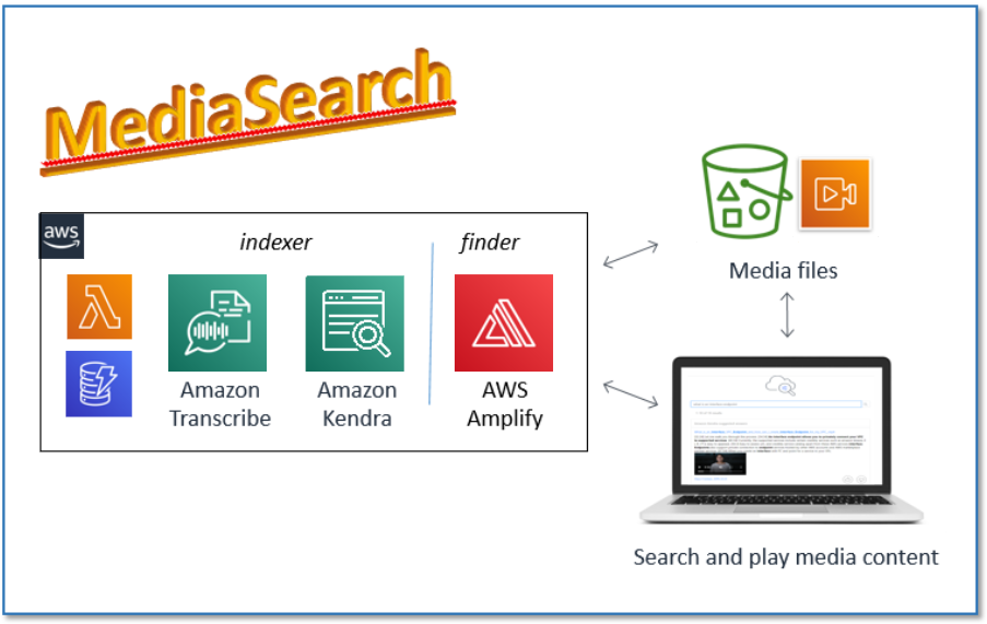
The first component, the MediaSearch indexer, finds and transcribes audio and video files stored in an Amazon Simple Storage Service (Amazon S3) bucket. It prepares the transcriptions by embedding time markers at the start of each sentence, and it indexes each prepared transcription in a new or existing Amazon Kendra index. It runs the first time when you install it, and subsequently runs on an interval that you specify, maintaining the index to reflect any new, modified, or deleted files.

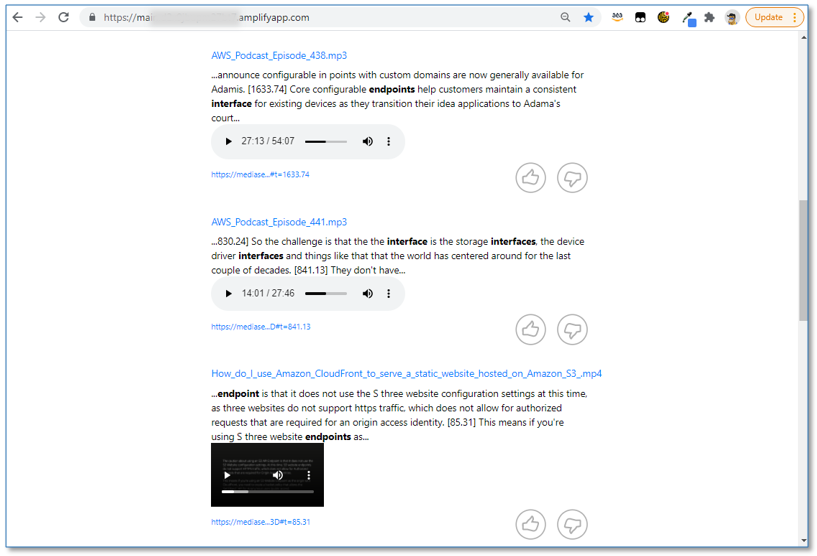
The second component, the MediaSearch finder, is a sample web search client that you use to search for content in your Amazon Kendra index. It has all the features of a standard Amazon Kendra search page, but it also includes in-line embedded media players in the search result, so you can not only see the relevant section of the transcript, but also play the corresponding section from the original media without navigating away from the search page (see the following screenshot).

In the sections that follow, we discuss several topics:

  • How to deploy the solution to your AWS account
  • How to use it to index and search sample media files
  • How to use the solution with your own media files
  • How the solution works under the hood
  • The costs involved
  • How to monitor usage and troubleshoot problems
  • Options to customize and tune the solution
  • How to uninstall and clean up when you’re done experimenting

Deploy the MediaSearch solution

In this section, we walk through deploying the two solution components: the indexer and the finder. We use an AWS CloudFormation stack to deploy the necessary resources in the us-east-1 (N. Virginia) AWS Region.

The source code is available in our GitHub repository. Follow the directions in the README to deploy MediaSearch to additional Regions supported by Amazon Kendra.

Deploy the indexer component

To deploy the indexer component, complete the following steps:

  1. Choose Launch Stack:
  2. Change the stack name if required to ensure that it’s unique.
  3. For ExistingIndexId, leave blank to create a new Amazon Kendra index (Developer Edition), otherwise provide the IndexId (not the index name) for an existing index in your account and Region (Amazon Kendra Enterprise Edition should be used for production workloads).
  4. For MediaBucket and MediaFolderPrefix, use the defaults initially to transcribe and index sample audio and video files.
  5. For now, use the default values for the other parameters.
  6. Select the acknowledgement check boxes, and choose Create stack.
  7. When the stack is created (after approximately 15 minutes), choose the Outputs tab, and copy the value of IndexId—you need it to deploy the finder component in the next step.

The newly installed indexer runs automatically to find, transcribe, and index the sample audio and video files. Later you can provide a different bucket name and prefix to index your own media files. If you have media files in multiple buckets, you can deploy multiple instances of the indexer, each with a unique stack name.

Deploy the finder component

To deploy the finder web application component, complete the following steps:

  1. Choose Launch Stack:
  2. For IndexId, use the Amazon Kendra index copied from the MediaSearch indexer stack outputs.
  3. For MediaBucketNames, use the default initially to allow the search page to access media files from the sample file bucket.
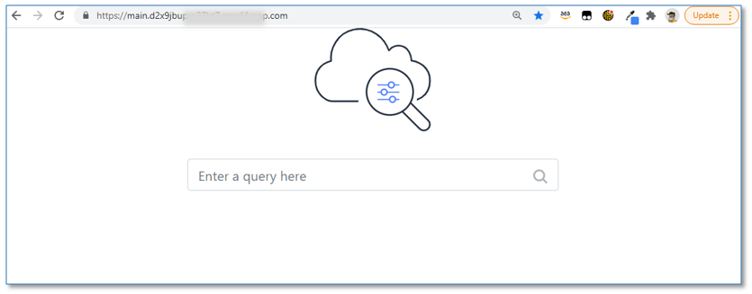
  4. When the stack is created (after approximately 5 minutes), choose the Outputs tab and use the link for MediaSearchFinderURL to open the new media search application page in your browser.

If the application isn’t ready when you first open the page, don’t worry! The initial application build and deployment (using AWS Amplify) takes about 10 minutes, so it will work when you try again a little later. If for any reason the application still doesn’t open, refer to the README in the GitHub repo for troubleshooting steps.

And that’s all there is to the deployment! Next, let’s run some search queries to see it in action.

Test with the sample media files

By the time the MediaSearch finder application is deployed and ready to use, the indexer should have completed processing the sample media files (selected AWS Podcast episodes and AWS Knowledge center videos). You can now run your first MediaSearch query.

  1. Open the MediaSearch finder application in your browser as described in the previous section.
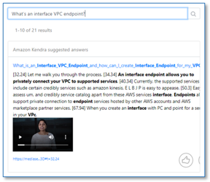
  2. In the query box, enter What’s an interface VPC Endpoint?

The query returns multiple results, sourced from the transcripts of the sample media files.

  1. Observe the time markers at the beginning of each sentence in the answer text. This indicates where the answer is to be found in the original media file.
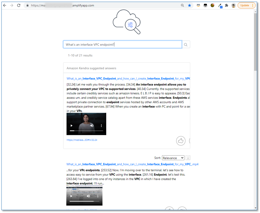
  2. Use the embedded video player to play the original video inline. Observe that the media playback starts at the relevant section of the video based on the time marker.
  3. To play the video full screen in a new browser tab, use the Fullscreen menu option in the player, or choose the media file hyperlink shown above the answer text.
  4. Choose the video file hyperlink (right-click), copy the URL, and paste it into a text editor. It looks something like the following:
https://mediasearchtest.s3.amazonaws.com/mediasamples/What_is_an_Interface_VPC_Endpoint_and_how_can_I_create_Interface_Endpoint_for_my_VPC_.mp4?AWSAccessKeyId=ASIAXMBGHMGZLSYWJHGD&Expires=1625526197&Signature=BYeOXOzT585ntoXLDoftkfS4dBU%3D&x-amz-security-token=.... #t=253.52

This is a presigned S3 URL that provides your browser with temporary read access to the media file referenced in the search result. Using presigned URLs means you don’t need to provide permanent public access to all of your indexed media files.

  1. Scroll down the page, and observe that some search results are from audio (MP3) files, and some are from video (MP4) files.

You can mix and match media types in the same index. You could include other data source types as well, such as documents, webpages, and other file types supported by available Amazon Kendra data sources, and search across them all, allowing Amazon Kendra to find the best content to answer your query.

  1. Experiment with additional queries, such as What does a solutions architect do? or What is Kendra?, or try your own questions.

Index and search your own media files

To index media files stored in your own S3 bucket, replace the MediaBucket and MediaFolderPrefix parameters with your own bucket name and prefix when you install or update the indexer component stack, and modify the MediaBucketNames parameter with your own bucket name when you install or update the finder component stack.

  1. Create a new MediaSearch indexer stack using an existing Amazon Kendra IndexId to add files stored in the new location. To deploy a new indexer, follow the directions in the Deploy the indexer component section in this post, but this time replace the defaults to specify the media bucket name and prefix for your own media files.
  2. Alternatively, update an existing MediaSearch indexer stack to replace the previously indexed files with files from the new location:
    1. Select the stack on the CloudFormation console, choose Update, then Use current template, then Next.
    2. Modify the media bucket name and prefix parameter values as needed.
    3. Choose Next twice, select the acknowledgement check box, and choose Update stack.
  3. Update an existing MediaSearch finder stack to change bucket names or add additional bucket names to the MediaBucketNames parameter.

When the MediaSearch indexer stack is successfully created or updated, the indexer automatically finds, transcribes, and indexes the media files stored in your S3 bucket. When it’s complete, you can submit queries and find answers from the audio tracks of your own audio and video files.

You have the option to provide metadata for any or all of your media files. Use metadata to assign values to index attributes for sorting, filtering, and faceting your search results, or to specify access control lists to govern access to the files. Metadata files can be in the same S3 folder as your media files (default), or in a parallel folder structure specified by the optional indexer parameter MetadataFolderPrefix. For more information about how to create metadata files, see S3 document metadata.

You can also provide customized transcription options for any or all of your media files. This allows you to take full advantage of Amazon Transcribe features such as custom vocabularies, automatic content redaction, and custom language models. For more information, refer to the README in the GitHub repo.

How the MediaSearch solution works

Let’s take a quick look under the hood to see how the solution works, as illustrated in the following diagram.

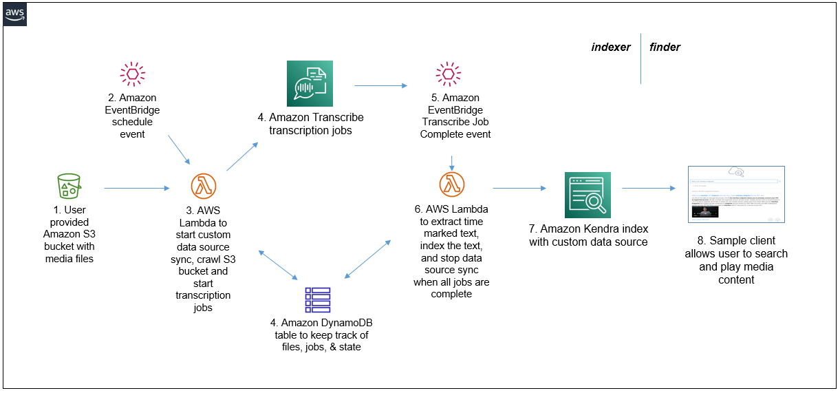
The MediaSearch solution has an event-driven serverless computing architecture with the following steps:

  1. You provide an S3 bucket containing the audio and video files you want to index and search.
  2. Amazon EventBridge generates events on a repeating interval (such as every 2 hours, every 6 hours, and so on)
  3. These events invoke an AWS Lambda function. The function is invoked initially when the CloudFormation stack is first deployed, and then subsequently by the scheduled events from EventBridge. An Amazon Kendra data source sync job is started. The Lambda function lists all the supported media files (FLAC, MP3, MP4, Ogg, WebM, AMR, or WAV) and associated metadata and Transcribe options stored in the user-provided S3 bucket.
  4. Each new file is added to the Amazon DynamoDB tracking table and submitted to be transcribed by a Transcribe job. Any file that has been previously transcribed is submitted for transcription again only if it has been modified since it was previously transcribed, or if associated Transcribe options have been updated. The DynamoDB table is updated to reflect the transcription status and last modified timestamp of each file. Any tracked files that no longer exist in the S3 bucket are removed from the DynamoDB table and from the Amazon Kendra index. If no new or updated files are discovered, the Amazon Kendra data source sync job is immediately stopped. The DynamoDB table holds a record for each media file with attributes to track transcription job names and status, and last modified timestamps.
  5. As each Transcribe job completes, EventBridge generates a Job Complete event, which invokes an instance of another Lambda function.
  6. The Lambda function processes the transcription job output, generating a modified transcription that has a time marker inserted at the start of each sentence. This modified transcription is indexed in Amazon Kendra, and the job status for the file is updated in the DynamoDB table. When the last file has been transcribed and indexed, the Amazon Kendra data source sync job is stopped.
  7. The index is populated and kept in sync with the transcriptions of all the media files in the S3 bucket monitored by the MediaSearch indexer component, integrated with any additional content from any other provisioned data sources. The media transcriptions are used by Amazon Kendra’s intelligent query processing, which allows users to find content and answers to their questions.
  8. The sample finder client application enhances users’ search experience by embedding an inline media player with each Amazon Kendra answer that is based on a transcribed media file. The client uses the time markers embedded in the transcript to start media playback at the relevant section of the original media file.

Estimate costs

In addition to Amazon S3 costs associated with storing your media, the MediaSearch solution incurs usage costs from Amazon Kendra and Transcribe. Additional minor (usually not significant) costs are incurred by the other services mentioned after free tier allowances have been used. For more information, see the pricing documentation for Amazon Kendra, Transcribe, Lambda, DynamoDB, and EventBridge.

Pricing example: Index the sample media files

The sample dataset has 25 media files—13 audio podcast and 12 video files—containing a total of around 480 minutes or 29,000 seconds of audio.

If you don’t provide an existing Amazon Kendra IndexId when you install MediaSearch, a new Amazon Kendra Developer Edition index is automatically created for you so you can test the solution. After you use your free tier allowance (up to 750 hours in the first 30 days), the index costs $1.125 per hour.

Transcribe pricing is based on the number of seconds of audio transcribed, with a free tier allowance of 60 minutes of audio per month for the first 12 months. After the free tier is used, the cost is $0.00040 for each second of audio transcribed. If you’re no longer free tier eligible, the cost to transcribe the sample files is as follows:

  • Total seconds of audio = 29,000
  • Transcription price per second = $0.00040
  • Total cost for Transcribe = [number of seconds] x [cost per second] = 29,000 x $0.00040 = $11.60

Monitor and troubleshoot

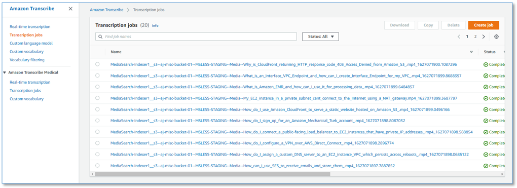
To see the details of each media file transcript job, navigate to the Transcription jobs page on the Transcribe console.

Each media file is transcribed only one time, unless the file is modified. Modified files are re-transcribed and re-indexed to reflect the changes.

Choose any transcription job to review the transcription and examine additional job details.

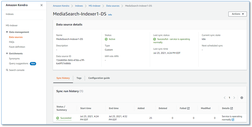
On the Indexes page of the Amazon Kendra console, choose the index used by MediaSearch to examine the index details.

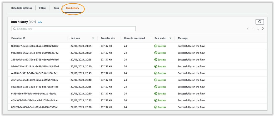
Choose Data sources in the navigation pane to examine the MediaSearch indexer data source, and observe the data source sync run history. The data source syncs when the indexer runs every interval specified in the CloudFormation stack parameters when you deployed or last updated the solution.

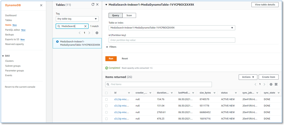
On the DynamoDB console, choose Tables in the navigation pane. Use your MediaSearch stack name as a filter to display the MediaSearch DynamoDB table, and examine the items showing each indexed media file and corresponding status. The table has one record for each media file, and contains attributes with information about the file and its processing status.

On the Functions page of the Lambda console, use your MediaSearch stack name as a filter to list the two MediaSearch indexer functions described earlier.

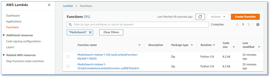
Choose either of the functions to examine the function details, including environment variables, source code, and more. Choose Monitor & View logs in CloudWatch to examine the output of each function invocation and troubleshoot any issues.

Customize and enhance the solution

You can fork the MediaSearch GitHub repository, enhance the code, and send us pull requests so we can incorporate and share your improvements!

The following are a few suggestions for features you might want to implement:

Clean up

When you’re finished experimenting with this solution, clean up your resources by using the AWS CloudFormation console to delete the indexer and finder stacks that you deployed. This deletes all the resources, including any Amazon Kendra indexes that were created by deploying the solution. Pre-existing indexes aren’t deleted. However, media files that were indexed by the solution are removed from the pre-existing index when you delete the indexer stack.

Conclusion

The combination of Amazon Transcribe and Amazon Kendra enable a scalable, cost-effective solution to make your media files discoverable. You can use the content of your media files to find accurate answers to your users’ questions, whether they’re from text documents or media files, and consume them in their native format. In other words, this solution is a leap in bringing media files on par with text documents as containers of information.

The sample MediaSearch application is provided as open source—use it as a starting point for your own solution, and help us make it better by contributing back fixes and features via GitHub pull requests. For expert assistance, AWS Professional Services and other Amazon partners are here to help.

We’d love to hear from you. Let us know what you think in the comments section, or using the issues forum in the MediaSearch GitHub repository.


About the Authors

Bob StrahanBob Strahan is a Principal Solutions Architect in the AWS Language AI Services team.


Abhinav JawadekarAbhinav Jawadekar is a Senior Partner Solutions Architect at Amazon Web Services. Abhinav works with AWS Partners to help them in their cloud journey.


Read More

Detect anomalies in operational metrics using Dynatrace and Amazon Lookout for Metrics

Organizations of all sizes and across all industries gather and analyze metrics or key performance indicators (KPIs) to help their businesses run effectively and efficiently. Operational metrics are used to evaluate performance, compare results, and track relevant data to improve business outcomes. For example, you can use operational metrics to determine application performance (the average time it takes to render a page for an end user) or application availability (the duration of time the application was operational). One challenge that most organizations face today is detecting anomalies in operational metrics, which are key in ensuring continuity of IT system operations.

Traditional rule-based methods are manual and look for data that falls outside of numerical ranges that have been arbitrarily defined. An example of this is an alert when transactions per hour fall below a certain number. This results in false alarms if the range is too narrow, or missed anomalies if the range is too broad. These ranges are also static. They don’t change based on evolving conditions like the time of the day, day of the week, seasons, or business cycles. When anomalies are detected, developers, analysts, and business owners can spend weeks trying to identify the root cause of the change before they can take action.

Amazon Lookout for Metrics uses machine learning (ML) to automatically detect and diagnose anomalies without any prior ML experience. In a couple of clicks, you can connect Lookout for Metrics to popular data stores like Amazon Simple Storage Service (Amazon S3), Amazon Redshift, and Amazon Relational Database Service (Amazon RDS), as well as third-party software as a service (SaaS) applications (such as Salesforce, Dynatrace, Marketo, Zendesk, and ServiceNow) via Amazon AppFlow and start monitoring metrics that are important to your business.

This post demonstrates how you can connect to your IT operational infrastructure monitored by Dynatrace using Amazon AppFlow and set up an accurate anomaly detector across metrics and dimensions using Lookout for Metrics. The solution allows you to set up a continuous anomaly detector and optionally set up alerts to receive notifications when anomalies occur.

Lookout for Metrics integrates seamlessly with Dynatrace to detect anomalies within your operational metrics. Once connected, Lookout for Metrics uses ML to start monitoring data and metrics for anomalies and deviations from the norm. Dynatrace enables monitoring of your entire infrastructure, including your hosts, processes, and network. You can perform log monitoring and view information such as the total traffic of your network, the CPU usage of your hosts, the response time of your processes, and more.

Amazon AppFlow is a fully managed service that provides integration capabilities by enabling you to transfer data between SaaS applications like Datadog, Salesforce, Marketo, and Slack and AWS services like Amazon S3 and Amazon Redshift. It provides capabilities to transform, filter, and validate data to generate enriched and usable data in a few easy steps.

Solution overview

In this post, we demonstrate how to integrate with an environment monitored by Dynatrace and detect anomalies in the operation metrics. We also determine how application availability and performance (resource contention) were impacted.

The source data is a cluster of Amazon Elastic Compute Cloud (Amazon EC2) instances that is monitored by Dynatrace. Each EC2 instance is installed with Dynatrace OneAgent to collect all monitored telemetry data (CPU utilization, memory, network utilization, and disk I/O). Amazon AppFlow enables you to securely integrate SaaS applications like Dynatrace and automate data flows, while providing options to configure and connect to such services natively from the AWS Management Console or via API. In this post, we focus on connecting to Dynatrace as our source and Lookout for Metrics as the target, both of which are natively supported applications in Amazon AppFlow.

The solution enables you to create an Amazon AppFlow data flow from Dynatrace to Lookout for Metrics. You can then use Lookout for Metrics to detect any anomalies in the telemetry data, as shown in the following diagram. Optionally, you can send automated anomaly alerts to AWS Lambda functions, webhooks, or Amazon Simple Notification Service (Amazon SNS) topics.

The following are the high-level steps to implement the solution:

  1. Set up Amazon AppFlow integration with Dynatrace.
  2. Create an anomaly detector with Lookout for Metrics.
  3. Add a dataset to the detector and integrate Dynatrace metrics.
  4. Activate the detector.
  5. Create an alert.
  6. Review the detector and data flow status.
  7. Review and analyze any anomalies.

Set up Amazon AppFlow integration with Dynatrace

To set up the data flow, complete the following steps:

  1. On the Amazon AppFlow console, choose Create flow.
  2. For Flow name, enter a name.
  3. For Flow description, enter an optional description.
  4. In the Data encryption section, you can choose or create an AWS Key Management Service (AWS KMS) key.
  5. Choose Next.
  6. For Source name, choose Dynatrace.
  7. For Choose Dynatrace Connection, choose the connection you created.
  8. For Choose Dynatrace object, choose Problems (this is the only object supported as of this writing).

For more information about Dynatrace problems, see Problem overview page.

  1. For Destination name, choose Amazon Lookout for Metrics.
  2. For API token, generate an API token from the Dynatrace console.
  3. For Subdomain, enter your Dynatrace portal URL address.
  4. For Data encryption, choose the AWS KMS key.
  5. For Connection Name, enter a name.
  6. Choose Connect.
  7. For Flow trigger, select Run flow on schedule.
  8. For Repeats, choose Minutes (alternatively, you can choose hourly or daily).
  9. Set the trigger to repeat every 5 minutes.
  10. Enter a starting time.
  11. Enter a start date.

Dynatrace requires a between date range filter to be set.

  1. For Field name, choose Date range.
  2. For Condition, choose is between.
  3. For Criteria 1, choose your start date.
  4. For Criteria 2, choose your end date.
  5. Review your settings and choose Create flow.

Create an anomaly detector with Lookout for Metrics

To create your anomaly detector, complete the following steps:

  1. On the Lookout for Metrics console, choose Create detector.
  2. For Detector name, enter a name.
  3. For Description, enter an optional description.
  4. For Interval, choose the time between each analysis. This should match the interval set on the flow.
  5. For Encryption, create or choose an existing AWS KMS key.
  6. Choose Create.

Add a dataset to the detector and integrate Dynatrace metrics

The next step in activating your anomaly detector is to add a dataset and integrate the Dynatrace metrics.

  1. On the detector details, choose Add a dataset.
  2. For Name, enter the data source name.
  3. For Description, enter an optional description.
  4. For Timezone, choose the time zone relevant to your dataset. This should match the time zone used in Amazon AppFlow (which picks up from the browser).
  5. For Datasource, choose Dynatrace.
  6. For Amazon AppFlow flow, choose the flow that you created.
  7. For Permissions, choose a service role.
  8. Choose Next.
  9. For Map fields, the detector tracks 5 measures; in this example I choose impactLevel and hasRootCause.

The map fields are the primary fields that the detector monitors. The fields that are relevant to monitor from an operational KPI should be considered.

  1. For Dimensions, the detector creates segments in measure values. For this post, I choose severityLevel.
  2. Review the settings and choose Save dataset.

Activate the detector

You’re now ready to activate the newly created detector.

Create an alert

You can create an alert to send automated anomaly alerts to Lambda functions; webhooks; cloud applications like Slack, PagerDuty, and DataDog; or to SNS topics with subscribers that use SMS, email, or push notifications.

  1. On the detector details, choose Add alerts.
  2. For Alert Name, enter the name.
  3. For Sensitivity threshold, enter a threshold at which the detector sends anomaly alerts.
  4. For Channel, choose either Amazon SNS or Lambda as the notification method. For this post, I use Amazon SNS.
  5. For SNS topic, create or choose an existing SNS topic.
  6. For Service role, choose an execution role.
  7. Choose Add alert.

Review the detector and flow status

On the Run history tab, you can confirm that the flows are running successfully for the interval chosen.

On the Detector log tab, you can confirm that the detector records the results after each interval.

Review and analyze any anomalies

On the main detector page, choose View anomalies to review and analyze any anomalies.

On the Anomalies page, you can adjust the severity score on the threshold dial to filter anomalies above a given score.

The following analysis represents the severity level and impacted metrics. The graph suggests anomalies detected by the detector with the availability and resource contention being impacted. The anomaly was detected on June 28 at 14:30 PDT and has a severity score of 98, indicating a high severity anomaly that needs immediate attention.

Lookout for Metrics also allows you to provide real-time feedback on the relevance of the detected anomalies, which enables a powerful human-in-the-loop mechanism. This information is fed back to the anomaly detection model to improve its accuracy continuously, in near-real time.

Conclusion

Anomaly detection can be very useful in identifying anomalies that could signal potential issues within your operational environment. Timely detection of anomalies can aid in troubleshooting, help avoid loss in revenue, and help maintain your company’s reputation. Lookout for Metrics automatically inspects and prepares the data, selects the best-suited ML algorithm, begins detecting anomalies, groups related anomalies together, and summarizes potential root causes.

To get started with this capability, see Amazon Lookout for Metrics. You can use this capability in all Regions where Lookout for Metrics is publicly available. For more information about Region availability, see AWS Regional Services.


About the Author

Sumeeth Siriyur is a Solutions Architect based out of AWS, Sydney. He is passionate about infrastructure services and uses AI services to influence IT infrastructure observability and management. In his spare time, he likes binge-watching and works to continually improve his outdoor sports.

Read More

Accenture promotes machine learning growth with world’s largest private AWS DeepComposer Battle of the Bands League

Accenture is known for pioneering innovative solutions to achieve customer success by using artificial intelligence (AI) and machine learning (ML) powered solutions with AWS services. To keep teams updated with latest ML services, Accenture seeks to gamify hands-on learning. One such event, AWS DeepComposer Battle of the Bands, hosted by Accenture, is the world’s first and largest global league.

Accenture’s league spanned 16 global regions and 55 countries, with each location competing for global superstardom and a real-life gold record! With around 500 bands in the competition, Accenture employees from different skills and domain knowledge proved themselves as aspiring ML musicians, generating a playlist of 150 original songs using AWS DeepComposer. There was no shortage of fans either, with thousands of votes being cast by supportive colleagues and teammates.

Why an AWS DeepComposer Battle of Bands and why now?

According to a recent Gartner report, “Despite the global impact of COVID-19, 47% of AI investments were unchanged since the start of the pandemic and 30% of organizations actually planned to increase such investments”. Additionally, there have been few opportunities in this pandemic to share a fun and enjoyable experience with our teammates, let alone colleagues around the globe.

Accenture and their Amazon Business Group are always looking for unique and exciting ways to help employees up-skill in the latest and greatest tech. Being inspired by their massively successful annual AWS DeepRacer Grand Prix, Accenture switched out the racetrack for the big stage and created their own Battle of the Bands using AWS DeepComposer.

This Battle of the Bands brought together fans and bands from around the globe, generating thousands of views, shares, votes, and opportunities to connect, laugh, and smile together.

Education was Accenture’s number one priority when crafting the competition. The goal was to expose those unfamiliar with AWS or ML to a fun and approachable experience that would increase their confidence with this technology and start them down a path of greater learning. According to registration metrics, around half of all participants were working with AWS and ML hands-on for the first time. Participants have shared that this competition inspired them to learn more about both AWS and ML. Some feedback received included:

“I enjoyed doing something creative and tackling music, which I had no experience with previously.”

“It was fun trying to make a song with the tool and to learn about other ML techniques.”

“I was able to feel like a musician even though I don’t know much about music composition.”

A hall of fame alliance

Accenture and AWS have always demonstrated a great alliance. In 2019, Accenture hosted one of the world’s largest private AWS DeepRacer Leagues. In 2021, multiple individuals and groups participated in the AWS DeepComposer Battle of the Bands League. These bands were able to create a video to go along with their song submission, allowing for more creative freedom and a chance to stand out from the crowd. Some bands made artistic music videos, others saw an opportunity to make something funny and share laughs around the world. Going above and beyond, one contestant turned their AWS DeepComposer competition into a sing-along training video for Accenture’s core values, while another dedicated their video to honoring “sheroes” and famous women in tech.

The dedication of Accenture’s bands to the spirit of the competition really showed in the array of pun-filled band names such as “Doggo-as-a-service,” “The Oracles,” “Anna and the AlgoRhythms,” and “#000000 Sabbath.”

AWS offers a portfolio of educational devices—AWS DeepLens, AWS DeepRacer, and AWS DeepComposer—designed for developers of all skill levels to learn the fundamentals of ML in fun and practical ways. The hands-on nature of AWS AI devices makes them great tools to engage and educate employees.

Accelerating innovation with the Accenture AWS Business Group

By working with the Accenture AWS Business Group (AABG), you can learn from the resources, technical expertise, and industry knowledge of two leading innovators, helping you accelerate the pace of innovation to deliver disruptive products and services. The AABG helps you ideate and innovate cloud solutions through rapid prototype development.

Connect with our team at accentureaws@amazon.com to learn how to use and accelerate ML in your products and services.

You can also organize your own event. To learn more about AWS DeepComposer events, see AWS DeepRacer Community Blog and also check out blog on How to run an AI powered musical challenge: “AWS DeepComposer Got Talent” to learn more about how to host your first event with AWS DeepComposer.

About Accenture

Accenture is a global professional services company with leading capabilities in digital, cloud and security. Combining unmatched experience and specialized skills across more than 40 industries, we offer Strategy and Consulting, Interactive, Technology and Operations services — all powered by the world’s largest network of Advanced Technology and Intelligent Operations centers. Our 569,000 people deliver on the promise of technology and human ingenuity every day, serving clients in more than 120 countries. We embrace the power of change to create value and shared success for our clients, people, shareholders, partners and communities. Visit us at www.accenture.com.

Copyright © 2021 Accenture. All rights reserved. Accenture and its logo are trademarks of Accenture.

This document is produced by consultants at Accenture as general guidance. It is not intended to provide specific advice on your circumstances. If you require advice or further details on any matters referred to, please contact your Accenture representative.

This document makes descriptive reference to trademarks that may be owned by others. The use of such trademarks herein is not an assertion of ownership of such trademarks by Accenture and is not intended to represent or imply the existence of an association between Accenture and the lawful owners of such trademarks. No sponsorship, endorsement, or approval of this content by the owners of such trademarks is intended, expressed, or implied.

Accenture provides the information on an “as-is” basis without representation or warranty and accepts no liability for any action or failure to act taken in response to the information contained or referenced in this publication.


About the Authors

Marc DeMory is a senior emerging tech consultant with Accenture’s Chicago Liquid Studio, focusing on rapid-prototyping and cloud-native development in the fields of Machine Learning, Computer Vision, Automation, and Extended Reality.


Sameer Goel is a Sr. Solutions Architect in Netherlands, who drives customer success by building prototypes on cutting-edge initiatives. Prior to joining AWS, Sameer graduated with a master’s degree from NEU Boston, with a concentration in data science. He enjoys building and experimenting with AI/ML projects on Raspberry Pi.


Maryam rezapoor is a Senior Product Manager with AWS DeepLabs team based in Santa Clara, CA. She works on developing products to put Machine Learning in the hands of everyone. She loves hiking through the US national parks and is currently training for 1-day Grand Canyon Rim to Rim hike. She is a fan of Metallica and Evanescence. The drummer, Lars Ulrich, has inspired her to pick up those sticks and play drum while singing “nothing else matters.”

Read More

Cattle-ist for the Future: Plainsight Revolutionizes Livestock Management with AI

Computer vision and edge AI are looking beyond the pasture.

Plainsight, a San Francisco-based startup and NVIDIA Metropolis partner, is helping the meat processing industry improve its operations — from farms to forks. By pairing Plainsight’s vision AI platform and NVIDIA GPUs to develop video analytics applications, the company’s system performs precision livestock counting and health monitoring.

With animals such as cows that look so similar, frequently shoulder-to-shoulder and moving quickly, inaccuracies in livestock counts are common in the cattle industry, and often costly.

On average, the cost of a cow in the U.S. is between $980 and $1,200, and facilities process anywhere between 1,000 to 5,000 cows per day. At this scale, even a small percentage of inaccurate counts equates to hundreds of millions of dollars in financial losses, nationally.

“By applying computer vision powered by edge AI and NVIDIA Metropolis, we’re able to automate what has traditionally been a very manual process and remove the uncertainty that comes with human counting,” said Carlos Anchia, CEO of Plainsight. “Organizations begin to optimize existing revenue streams when accuracy can be operationally efficient.”

Plainsight is working with JBS USA, one of the world’s largest food companies, to integrate vision AI into its operational processes. Vision AI-powered cattle counting was among the first solutions to be implemented.

At JBS, cows are counted by fixed-position cameras, connected via a secured private network to Plainsight’s vision AI edge application, which detects, tracks and counts the cows as they move past.

Plainsight’s models count livestock with over 99.5 percent accuracy — about two percentage points better than manual livestock counting by humans in the same conditions, according to the company.


For a vision AI solution to be widely adopted by an organization, the accuracy must be higher than humans performing the same activity. By monitoring and tracking each individual animal, the models simplify an otherwise complex process.

Highly robust and accurate computer vision models are only a portion of the cattle counting solution. Through continued collaboration with JBS’s operations and innovation teams, Plainsight provided a path to the digital transformation required to more accurately provide accountability when receiving livestock at scale and thus ensure that the payment for livestock received is as accurate as possible.

Higher Accuracy with GPMoos

For JBS, the initial proof of value involved building models and deploying on an NVIDIA Jetson AGX Xavier Developer Kit.

After quickly achieving nearly 100 percent accuracy levels with their models, the teams moved into a full pilot phase. To augment the model to handle new and often challenging environmental conditions, Plainsight’s AI platform was used to quickly and easily annotate, build and deploy model improvements in preparation for a nationwide rollout.

As a member partner of NVIDIA Metropolis, an application framework that brings visual data and AI together, Plainsight continues to develop and improve models and AI pipelines to enable a national rollout with the U.S. division of JBS.

There, Plainsight uses a technology stack built on the NVIDIA EGX platform, incorporating NVIDIA-Certified Systems with NVIDIA T4 GPUs. Plainsight’s application processes multiple video streams per GPU in real time to count and monitor livestock as part of managing the accounting of livestock when received.

“Innovation is fundamental to the JBS culture, and the application of AI technology to improve efficiencies for daily work routines is important,” said Frederico Scarin do Amaral, Senior Manager Business Solutions of JBS USA. “Our partnership with Plainsight enhances the work of our team members and ensures greater accuracy of livestock count, improving our operations and efficiency, as well as allowing for continual improvements of animal welfare.”

Milking It

Inaccurate counting is only part of the problem the industry faces, however. Visual inspection of livestock is arduous and error-prone, causing late detection of diseases and increasing health risks to other animals.

The same symptoms humans can identify by looking at an animal, such as gait and abnormal behavior, can be approximated by computer vision models built, trained and managed through Plainsight’s vision AI platform.

The models identify symptoms of particular diseases, based on the gait and anomalies in how livestock behave when exiting transport vehicles, in a pen or in feeding areas.

“The cameras are an unblinking source of truth that can be very useful in identifying and alerting to problems otherwise gone unnoticed,” said Anchia. “The combination of vision AI, cameras and Plainsight’s AI platform can help enhance the vigilance of all participants in the cattle supply chain so they can focus more on their business operations and animal welfare improvements as opposed to error-prone manual counting.”

Legen-Dairy

In addition to a variety of other smart agriculture applications, Plainsight is using its vision AI platform to monitor and track cattle on the blockchain as digital assets.

The company is engaged in a first-of-its-kind co-innovation project with CattlePass, a platform that generates a secure and unique digital record of individual livestock, also known as a non-fungible token, or NFT.

Plainsight is applying its advanced vision AI models and platform for monitoring cattle health. The suite of advanced technologies, including genomics, health and proof-of-life records, will provide 100 percent verifiable proof of ownership and transparency into a complete living record of the animal throughout its lifecycle.

Cattle ranchers will be able to store the NFTs in a private digital wallet while collecting and adding metadata: feed, heartbeat, health, etc. This data can then be shared with permissioned viewers such as inspectors, buyers, vets and processors.

The data will remain with each animal throughout its life through harvest, and data will be provided with a unique QR code printed on the beef packaging. This will allow for visibility into the proof of life and quality of each cow, giving consumers unprecedented knowledge about its origin.

The post Cattle-ist for the Future: Plainsight Revolutionizes Livestock Management with AI appeared first on The Official NVIDIA Blog.

Read More

Scale your Amazon Kendra index

Amazon Kendra is a fully managed, intelligent search service powered by machine learning. Amazon Kendra reimagines enterprise search for your websites and applications so your employees and customers can easily find the content they’re looking for. Using keyword or natural language queries, employees and customers can find the right content even when it’s scattered across multiple locations and content repositories within your organization.

Although Amazon Kendra is designed for large-scale search applications with millions of documents and thousands of queries per second, you can run smaller experiments to evaluate Amazon Kendra. You can run a proof of concept, or simply have a smaller workload and still use features that Amazon Kendra Enterprise Edition has to offer. On July 1, 2021, Amazon Kendra introduced new, smaller capacity units for smaller workloads. In addition, to promote experimentation, the price for Amazon Kendra Developer Edition was reduced by 55%.

Amazon Kendra Enterprise Edition capacity units

The base capacity for Amazon Kendra supports up to 100,000 documents and 8,000 searches per day, with adaptive bursting capability to better handle unpredictable query spikes. You can increase the query and the document capacity of your Amazon Kendra index through storage capacity units and query capacity units, and these can be updated independently from each other.

Storage capacity units offer scaling in increments of 100,000 documents (up to 30 GB storage), each. For example, if you need to index 1 million documents, you need nine storage capacity units (100,000 documents with base Amazon Kendra Enterprise Edition, and, 900,00 additional documents from the storage capacity units).

Query capacity units (QCUs) offer scaling increments of 8,000 searches for day, with built-in adaptive bursting. For example, if you need 16K queries per day (average QPS of 0.2) you can provision two units.

For more information about the maximum number of storage capacity units and query capacity units available for a single index, see Quotas for Amazon Kendra.

About capacity bursting

Amazon Kendra has a provisioned base capacity of one query capacity unit. You can use up to 8,000 queries per day with a minimum throughput of 0.1 queries per second (per query capacity unit).

An adaptive approach to handling unexpected traffic beyond the provisioned throughput is to use the built-in adaptive query bursting feature in Amazon Kendra. This allows you to apply unused query capacity to handle unexpected traffic. Amazon Kendra accumulates your unused queries at your provisioned queries per second rate, every second, up to the maximum number of queries you’ve provisioned for your Amazon Kendra index. These accumulated queries are automatically used to help handle unexpected traffic spikes above the currently allocated QPS capacity.

Optimal performance of adaptive query bursting can vary, depending on several factors such as your total index size, query complexity, accumulated unused queries, and overall load on your index. We recommend performing your own load tests to accurately measure bursting capacity.

Best practices

When dimensioning your Amazon Kendra index, you need to consider how many documents you’re indexing, how many queries you expect per day, how many queries per second you need to accommodate, and if you have usage patterns that require additional capacity due to sustained usage. You could also experience short peak times where you can accommodate brief periods of time for additional QPS requirements.

It’s therefore good practice to observe your query usage patterns for a few weeks, especially when the patterns are not easily predictable. This will allow you to define an optimal balance between using the built-in adaptive bursting capability for short, unsustained QPS peaks, and adding/removing capacity units to better handle longer, more sustained peaks and lows.

For information about visualizing and building a rough estimate of your usage patterns in Amazon Kendra, see Automatically scale Amazon Kendra query capacity units with Amazon EventBridge and AWS Lambda.

Amazon Kendra Enterprise Edition allows you to add document storage capacity in units of 100,000 documents with maximum storage of 30 GB. You can add and remove storage capacity at any time, but you can’t remove storage capacity beyond your used capacity (number of documents ingested or storage space used). We recommend estimating how often documents are added to your data sources in order to determine when to increase storage capacity in your Amazon Kendra through storage capacity units. You can monitor the document count with Amazon CloudWatch or on the Amazon Kendra console.

Queries per second represent the number of concurrent queries your Amazon Kendra index receives at a given time. If you’re replacing a search solution with Amazon Kendra, you should be able to retrieve this information from query logs. If you exceed your provisioned and bursting capacity, your request may receive a 400 HTTP status code (client error) with the message ThrottlingException. For example, using the AWS SDK for Python (Boto3), you may receive an exception like the following:

ThrottlingException: An error occurred (ThrottlingException) when calling the Query operation (reached max retries: 4)

For cases like this, Boto3 includes the retries feature, which retries the query call (in this case to Amazon Kendra) after obtaining an exception. If you aren’t using an AWS SDK, you may need to implement an error handling mechanism that, for example, could use exponential backoff to handle this error.

You can monitor your Amazon Kendra index queries with CloudWatch metrics. For example, you could follow the metric IndexQueryCount, which represents the number of index queries per minute. If you want to use the IndexQueryCount metric, you should divide that number by 60 to obtain the average queries per second. Additionally, you can get a report of the queries per second on the Amazon Kendra console, as shown in the following screenshot.

The preceding graph shows three patterns:

  • Peaks of ˜2.5 QPS during business hours, between 8 AM and 8 PM.
  • Sustained QPS usage over ˜0.5 QPS and below 1 QPS between 8 PM and 8 AM.
  • Less than 0.3 QPS usage on the weekend (Feb 7, 2021, was a Sunday and Feb 13,2021 was a Saturday)

Taking into account these capacity requirements, you could start defining your Amazon Kendra index additional capacity units as follows:

  • For the high usage times (between 8 AM and 8 PM Monday through Friday), your Amazon Kendra index adds 24 VQUs (each query capacity unit provides capacity for at least 0.1 QPS) which when added to the initial Amazon Kendra Enterprise Edition query capacity (0.1 QPS), can support 2.5 queries per second
  • For the second usage pattern (Monday through Friday from 8 PM until 8 AM), you add four VQUs, which when combined with your initial Amazon Kendra Enterprise Edition (0.1 QPS), provides capacity for 0.5 QPS.
  • For the weekends, you add two VQUs, provisioning capacity for 0.3 QPS.

The following table summarizes this configuration.

Period Additional VQUS Capacity (Without Bursting)
Mon – Fri 8 AM – 8 PM 24 2.5 QPS
Mon – Fri 8 PM – 8 AM 4 0.5 QPS
Sat – Sun 2 0.3 QPS

You can use this initial approach to define a baseline that needs to be reevaluated to ensure the right sizing of your Amazon Kendra resources.

It’s also important to keep in mind that query autocomplete capacity is defined by your query capacity. Query autocomplete capacity is calculated as five times the provisioned query capacity for an index with a base capacity of 2.5 calls per second. This means that if your Amazon Kendra index query capacity is below 0.6 QPS, you have 2.5 QPS for query autocomplete. If your Amazon Kendra index query capacity is above 0.6 QPS, your query autocomplete capacity is calculated as 2.5 times your current index query capacity.

Conclusion

In this blog post you learned how to estimate capacity and scale for your Amazon Kendra index.

Now it’s easier than ever to experience Amazon Kendra, with 750 hours of Free Tier and the new reduced price for Amazon Kendra Developer Edition. Get started, visit our workshop, or check out the AWS Machine Learning Blog.


About the Author

Dr. Andrew Kane is an AWS Principal Specialist Solutions Architect based out of London. He focuses on the AWS Language and Vision AI services, helping our customers architect multiple AI services into a single use-case driven solution. Before joining AWS at the beginning of 2015, Andrew spent two decades working in the fields of signal processing, financial payments systems, weapons tracking, and editorial and publishing systems. He is a keen karate enthusiast (just one belt away from Black Belt) and is also an avid home-brewer, using automated brewing hardware and other IoT sensors.


Tapodipta Ghosh is a Senior Architect. He leads the Content And Knowledge Engineering Machine Learning team that focuses on building models related to AWS Technical Content. He also helps our customers with AI/ML strategy and implementation using our AI Language services like Amazon Kendra.


Jean-Pierre Dodel leads product management for Amazon Kendra, a new ML-powered enterprise search service from AWS. He brings 15 years of Enterprise Search and ML solutions experience to the team, having worked at Autonomy, HP, and search startups for many years prior to joining Amazon four years ago. JP has led the Amazon Kendra team from its inception, defining vision, roadmaps, and delivering transformative semantic search capabilities to customers like Dow Jones, Liberty Mutual, 3M, and PwC.


Juan Bustos is an AI Services Specialist Solutions Architect at Amazon Web Services, based in Dallas, TX. Outside of work, he loves spending time writing and playing music as well as trying random restaurants with his family.

Read More

Archaeologist Digs Into Photogrammetry, Creates 3D Models With NVIDIA Technology

Archaeologist Daria Dabal is bringing the past to life, with an assist from NVIDIA technology.

Dabal works on various archaeological sites in the U.K., conducting field and post-excavation work. Over the last five years, photogrammetry — the use of photographs to create fully textured 3D models — has become increasingly popular in archaeology. Dabal has been expanding her skills in this area to create and render high-quality models of artifacts and sites.

With the help of her partner, Simon Kotowicz, Dabal is taking photogrammetry scans to the next level with a pair of NVIDIA graphics technologies.

Using NVIDIA RTX GPUs, Dabal can accelerate workflows to create and interact with 3D models, from recreating missing elements to adding animations or dropping them into VR. And with the NVIDIA Omniverse real-time collaboration and simulation platform, she can build stunning scenes around her projects using the platform’s library of existing assets.

All for the (Photo)Gram

Dabal quickly learned that good photogrammetry requires a good dataset. It’s important to take photos in the right pattern, so that every area of the site, monument or artifact is covered.

Once she has all the images she needs, Dabal builds the 3D models using Agisoft Metashape, a tool for photogrammetry pipelines. Dabal loads all her photos into the application, and the software turns that data into a point cloud, which is a rough collection of dots that represent the 3D model.

Recently, Dabal and Kotowicz were approached by The Flow State XR, a company that delivers immersive experiences and applications. They were tasked with a new photogrammetry project that rocked their world: creating a 3D model of The Crobar, an iconic, heavy-metal bar located in the heart of Soho in London.

The Flow State XR sent images of The Crobar to the duo, who used the photos to model the bar from scratch, then created texture maps using Adobe Photoshop, Illustrator and Substance Painter. Dabal and Kotowicz are currently finishing the 3D model, but once the project is complete, The Flow State XR plans to use it as an interactive mobile app and a VR hangout for music fans.

The Crobar VR scene. Image courtesy of Dabal.

RTX Shapes 3D Modeling Workflows

Dabal uses an NVIDIA Quadro RTX 4000 GPU to significantly speed up her 3D modeling and rendering workflows. Processing a sparse cloud model with her older generation GPU would take two days, she said. With the upgraded RTX card, a similar point cloud takes only 10 hours.

With NVIDIA RTX, the millions of points on a model can be rotated and zoomed much more easily. The team can also use their 4K monitor to view the models, which they couldn’t do previously because it was difficult to navigate around the point clouds.

Dabal and Kotowicz have also experienced faster performance in creative apps like Autodesk  3ds Max. They can iterate quicker and see textures in graphics without needing to render as often.

“The NVIDIA RTX card has helped us achieve the model we need much faster,” said Dabal. “We’re spending less time in front of the workstation, and we’re getting to the rendering stage a lot quicker now.”

Textured 3D model of the Neath Abbey Ironworks. Image courtesy of Dabal.

Omniverse Makes Space for Sharing Assets, Building Scenes 

Dabal got the chance to use the advanced features of NVIDIA Omniverse when she entered the first “Create With Marbles” design competition. After exploring the platform, Dabal sees great potential in how it will transform traditional workflows and images in archaeology.

Dabal’s submission for the NVIDIA Omniverse “Create With Marbles” design competition.

Currently, there isn’t a tool that enables archaeologists to quickly upload assets in one place, and share or collaborate with others on the same projects.

With an open platform like Omniverse, archaeologists have a virtual space where they can easily upload photogrammetry artifacts and share assets with one another, no matter what location they’re working from. Or they could place models in Omniverse and create a stunning scene by adding extra elements, like trees or farm fields.

“Right now, most archaeological 3D models look fake, floating in their black backgrounds. It would take too much time to add the extras, but it would be so easy in Omniverse,” said Dabal. “When I was in Omniverse, I really enjoyed taking premade objects and moving them around to create a scene. It was super easy.”

Dabal says that if archeologists had access to a library of extra assets, as well as all their own photogrammetry scans, “it would be game-changing.”

With Omniverse, archaeologists can share their projects with others around the world as well as simulate fire or weather conditions to bring their 3D models and sites to life.

Explore more of Dabal’s work, and learn more about NVIDIA RTX and NVIDIA Omniverse.

And join NVIDIA at SIGGRAPH, where we’ll showcase the technologies driving the future of graphics. We’ll announce the winners of the latest “Create With Marbles: Marvelous Machines” contest winner, and premiere a documentary highlighting how Omniverse was used to create the NVIDIA GTC 2021 keynote.

The post Archaeologist Digs Into Photogrammetry, Creates 3D Models With NVIDIA Technology appeared first on The Official NVIDIA Blog.

Read More

Ready for Prime Time: Plus to Deliver Autonomous Truck Systems Powered by NVIDIA DRIVE to Amazon

Your Amazon Prime delivery just got smarter.

Autonomous trucking company Plus recently signed a deal with Amazon to provide at least 1,000 self-driving systems to retrofit on the e-commerce giant’s delivery fleet. These systems are powered by NVIDIA DRIVE Xavier for high-performance, energy-efficient and centralized AI compute.

The agreement follows Plus’ announcement of going public via SPAC, or special acquisition company.

Amazon — which leads the U.S. e-tail market, counting $386 billion in net revenue in 2020 — has been investing heavily in autonomous and electric vehicle technology. Last year, it acquired robotaxi company and NVIDIA DRIVE ecosystem member Zoox for $1.3 billion.

These deals signal the transition to autonomous systems in both personal and commercial transportation at a massive scale.

An A-Plus Platform

The current generation PlusDrive autonomous trucking platform was developed for level 4 autonomous driving with a human driver still at the wheel, using NVIDIA DRIVE Xavier system-on-a-chip at its core.

Xavier is the first-ever production, automotive-grade SoC for autonomous capabilities. It incorporates six different types of processors, including a CPU, GPU, deep learning accelerator, programmable vision accelerator, image signal processor and stereo/optical flow accelerator.

Architected for safety, Xavier incorporates the redundancy and diversity necessary for safe autonomous operation.

This high-performance compute enables the PlusDrive system to perform surround perception with an array of radar, lidar and camera sensors, running a variety of deep neural networks simultaneously and in real time.

Trucking Ahead

Plus’s deal with Amazon is just the beginning of the march toward widespread autonomous delivery.

The self-driving company has already announced plans to transition to the next generation of AI compute, NVIDIA DRIVE Orin, beginning in 2022. Plus has received more than 7,000 orders and pre-orders for this upcoming system.

Additionally, Amazon has been granted a warrant to buy a 20 percent stake in Plus after they spend more than $150 million, opening up the possibility for even deeper integration of the company’s technology with the e-retailer’s delivery fleet.

And with NVIDIA DRIVE at their core, these autonomous systems will be able to handle the AI processing necessary to deliver safe, efficient and continuously improving trucks at scale.

The post Ready for Prime Time: Plus to Deliver Autonomous Truck Systems Powered by NVIDIA DRIVE to Amazon appeared first on The Official NVIDIA Blog.

Read More

Improved Detection of Elusive Polyps via Machine Learning

Posted by Yossi Matias, Vice President and Ehud Rivlin, Research Scientist, Google Research

With the increasing ability to consistently and accurately process large amounts of data, particularly visual data, computer-aided diagnostic systems are more frequently being used to assist physicians in their work. This, in turn, can lead to meaningful improvements in health care. An example of where this could be especially useful is in the diagnosis and treatment of colorectal cancer (CRC), which is especially deadly and results in over 900K deaths per year, globally. CRC originates in small pre-cancerous lesions in the colon, called polyps, the identification and removal of which is very successful in preventing CRC-related deaths.

The standard procedure used by gastroenterologists (GIs) to detect and remove polyps is the colonoscopy, and about 19 million such procedures are performed annually in the US alone. During a colonoscopy, the gastroenterologist uses a camera-containing probe to check the intestine for pre-cancerous polyps and early signs of cancer, and removes tissue that looks worrisome. However, complicating factors, such as incomplete detection (in which the polyp appears within the field of view, but is missed by the GI, perhaps due to its size or shape) and incomplete exploration (in which the polyp does not appear in the camera’s field of view), can lead to a high fraction of missed polyps. In fact, studies suggest that 22%–28% of polyps are missed during colonoscopies, of which 20%–24% have the potential to become cancerous (adenomas).

Today, we are sharing progress made in using machine learning (ML) to help GIs fight colorectal cancer by making colonoscopies more effective. In “Detection of Elusive Polyps via a Large Scale AI System”, we present an ML model designed to combat the problem of incomplete detection by helping the GI detect polyps that are within the field of view. This work adds to our previously published work that maximizes the coverage of the colon during the colonoscopy by flagging for GI follow-up areas that may have been missed. Using clinical studies, we show that these systems significantly improve polyp detection rates.

Incomplete Exploration
To help the GI detect polyps that are outside the field of view, we previously developed an ML system that reduces the rate of incomplete exploration by estimating the fractions of covered and non-covered regions of a colon during a colonoscopy. This earlier work uses computer vision and geometry in a technique we call colonoscopy coverage deficiency via depth, to compute segment-by-segment coverage for the colon. It does so in two phases: first computing depth maps for each frame of the colonoscopy video, and then using these depth maps to compute the coverage in real time.

The ML system computes a depth image (middle) from a single RGB image (left). Then, based on the computation of depth images for a video sequence, it calculates local coverage (right), and detects where the coverage has been deficient and a second look is required (blue color indicates observed segments where red indicates uncovered ones). You can learn more about this work in our previous blog post.

This segment-by-segment work yields the ability to estimate what fraction of the current segment has been covered. The helpfulness of such functionality is clear: during the procedure itself, a physician may be alerted to segments with deficient coverage, and can immediately return to review these areas, potentially reducing the rates of missed polyps due to incomplete exploration.

Incomplete Detection
In our most recent paper, we look into the problem of incomplete detection. We describe an ML model that aids a GI in detecting polyps that are within the field of view, so as to reduce the rate of incomplete detection. We developed a system that is based on convolutional neural networks (CNN) with an architecture that combines temporal logic with a single frame detector, resulting in more accurate detection.

This new system has two principal advantages. The first is that the system improves detection performance by reducing the number of false negatives detections of elusive polyps, those polyps that are particularly difficult for GIs to detect. The second advantage is the very low false positive rate of the system. This low false positive rate makes these systems more likely to be adopted in the clinic.

Examples of the variety of polyps detected by the ML system.

We trained the system on 3600 procedures (86M video frames) and tested it on 1400 procedures (33M frames). All the videos and metadata were de-identified. The system detected 97% of the polyps (i.e., it yielded 97% sensitivity) at 4.6 false alarms per procedure, which is a substantial improvement over previously published results. Of the false alarms, follow-up review showed that some were, in fact, valid polyp detections, indicating that the system was able to detect polyps that were missed by the performing endoscopist and by those who annotated the data. The performance of the system on these elusive polyps suggests its generalizability in that the system has learned to detect examples that were initially missed by all who viewed the procedure.

We evaluated the system performance on polyps that are in the field of view for less than five seconds, which makes them more difficult for the GI to detect, and for which models typically have much lower sensitivity. In this case the system attained a sensitivity that is about three times that of the sensitivity that the original procedure achieved. When the polyps were present in the field of view for less than 2 seconds, the difference was even more stark — the system exhibited a 4x improvement in sensitivity.

It is also interesting to note that the system is fairly insensitive to the choice of neural network architecture. We used two architectures: RetinaNet and  LSTM-SSD. RetinaNet is a leading technique for object detection on static images (used for video by applying it to frames in a consecutive fashion). It is one of the top performers on a variety of benchmarks, given a fixed computational budget, and is known for balancing speed of computation with accuracy. LSTM-SSD is a true video object detection architecture, which can explicitly account for the temporal character of the video (e.g., temporal consistency of detections, ability to deal with blur and fast motion, etc.). It is known for being robust and very computationally lightweight and can therefore run on less expensive processors. Comparable results were also obtained on the much heavier Faster R-CNN architecture. The fact that results are similar across different architectures implies that one can choose the network meeting the available hardware specifications.

Prospective Clinical Research Study
As part of the research reported in our detection paper we ran a clinical validation on 100 procedures in collaboration with Shaare Zedek Medical Center in Jerusalem, where our system was used in real time to help GIs. The system helped detect an average of one polyp per procedure that would have otherwise been missed by the GI performing the procedure, while not missing any of the polyps detected by the GIs, and with 3.8 false alarms per procedure. The feedback from the GIs was consistently positive.

We are encouraged by the potential helpfulness of this system for improving polyp detection, and we look forward to working together with the doctors in the procedure room to further validate this research.

Acknowledgements
The research was conducted by teams from Google Health and Google Research, Israel with support from Verily Life Sciences, and in collaboration with Shaare Zedek Medical Center. Verily is advancing this research via a newly established center in Israel, led by Ehud Rivlin. This research was conducted by Danny Veikherman, Tomer Golany, Dan M. Livovsky, Amit Aides, Valentin Dashinsky, Nadav Rabani, David Ben Shimol, Yochai Blau, Liran Katzir, Ilan Shimshoni, Yun Liu, Ori Segol, Eran Goldin, Greg Corrado, Jesse Lachter, Yossi Matias, Ehud Rivlin, and Daniel Freedman. Our appreciation also goes to several institutions and GIs who provided advice along the way and tested our system prototype. We would like to thank all of our team members and collaborators who worked on this project with us, including: Chen Barshai, Nia Stoykova, and many others.

Read More