When deploying Deep Learning models at scale, it is crucial to effectively utilize the underlying hardware to maximize performance and cost benefits. For production workloads requiring high throughput and low latency, the selection of the Amazon Elastic Compute Cloud (EC2) instance, model serving stack, and deployment architecture is very important. Inefficient architecture can lead to suboptimal utilization of the accelerators and unnecessarily high production cost.
In this post we walk you through the process of deploying FastAPI model servers on AWS Inferentia devices (found on Amazon EC2 Inf1 and Amazon EC Inf2 instances). We also demonstrate hosting a sample model that is deployed in parallel across all NeuronCores for maximum hardware utilization.
Solution overview
FastAPI is an open-source web framework for serving Python applications that is much faster than traditional frameworks like Flask and Django. It utilizes an Asynchronous Server Gateway Interface (ASGI) instead of the widely used Web Server Gateway Interface (WSGI). ASGI processes incoming requests asynchronously as opposed to WSGI which processes requests sequentially. This makes FastAPI the ideal choice to handle latency sensitive requests. You can use FastAPI to deploy a server that hosts an endpoint on an Inferentia (Inf1/Inf2) instances that listens to client requests through a designated port.
Our objective is to achieve highest performance at lowest cost through maximum utilization of the hardware. This allows us to handle more inference requests with fewer accelerators. Each AWS Inferentia1 device contains four NeuronCores-v1 and each AWS Inferentia2 device contains two NeuronCores-v2. The AWS Neuron SDK allows us to utilize each of the NeuronCores in parallel, which gives us more control in loading and inferring four or more models in parallel without sacrificing throughput.
With FastAPI, you have your choice of Python web server (Gunicorn, Uvicorn, Hypercorn, Daphne). These web servers provide and abstraction layer on top of the underlying Machine Learning (ML) model. The requesting client has the benefit of being oblivious to the hosted model. A client doesn’t need to know the model’s name or version that has been deployed under the server; the endpoint name is now just a proxy to a function that loads and runs the model. In contrast, in a framework-specific serving tool, such as TensorFlow Serving, the model’s name and version are part of the endpoint name. If the model changes on the server side, the client has to know and change its API call to the new endpoint accordingly. Therefore, if you are continuously evolving the version models, such as in the case of A/B testing, then using a generic Python web server with FastAPI is a convenient way of serving models, because the endpoint name is static.
An ASGI server’s role is to spawn a specified number of workers that listen for client requests and run the inference code. An important capability of the server is to make sure the requested number of workers are available and active. In case a worker is killed, the server must launch a new worker. In this context, the server and workers may be identified by their Unix process ID (PID). For this post, we use a Hypercorn server, which is a popular choice for Python web servers.
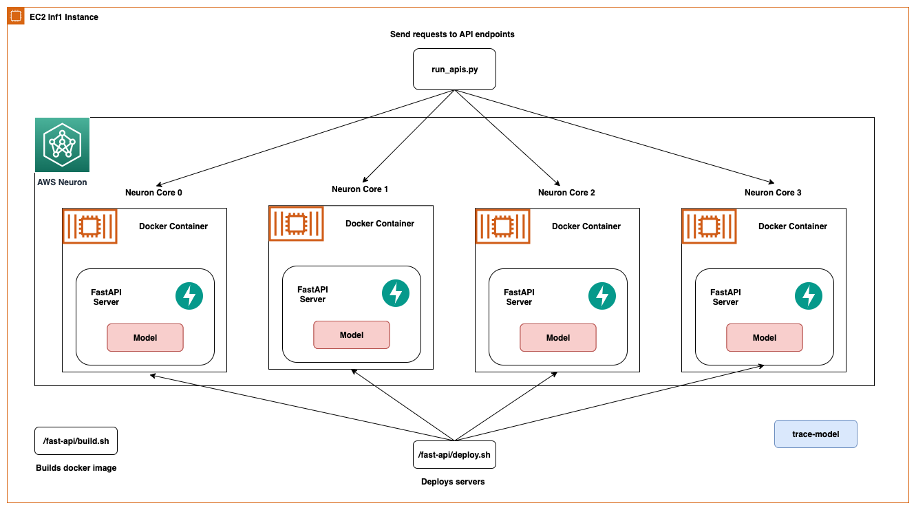
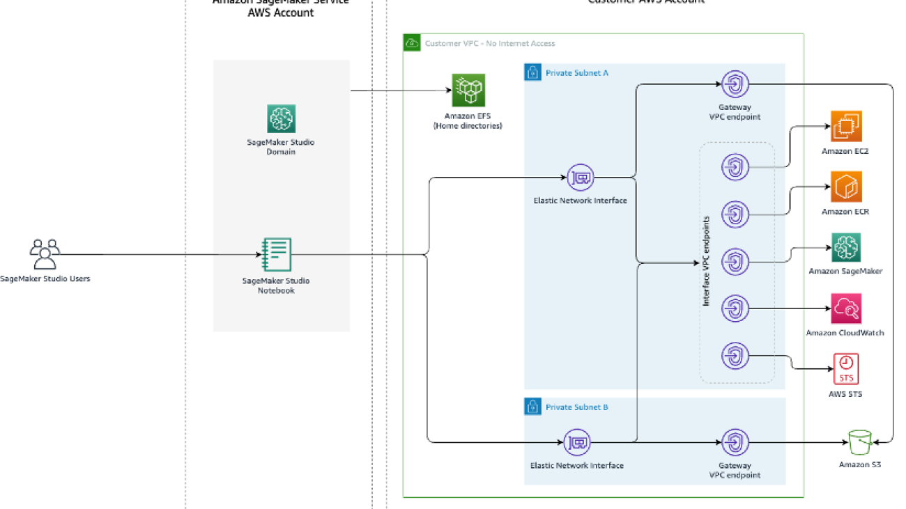
In this post, we share best practices to deploy deep learning models with FastAPI on AWS Inferentia NeuronCores. We show that you can deploy multiple models on separate NeuronCores that can be called concurrently. This setup increases throughput because multiple models can be inferred concurrently and NeuronCore utilization is fully optimized. The code can be found on the GitHub repo. The following figure shows the architecture of how to set up the solution on an EC2 Inf2 instance.
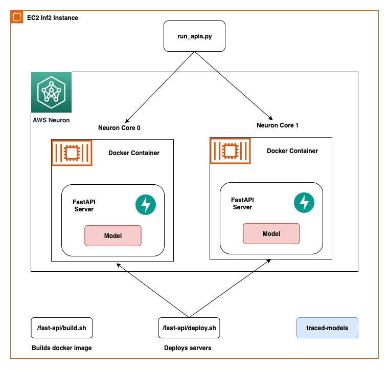
The same architecture applies to an EC2 Inf1 instance type except it has four cores. So that changes the architecture diagram a little bit.
AWS Inferentia NeuronCores
Let’s dig a little deeper into tools provided by AWS Neuron to engage with the NeuronCores. The following tables shows the number of NeuronCores in each Inf1 and Inf2 instance type. The host vCPUs and the system memory are shared across all available NeuronCores.
| Instance Size |
# Inferentia Accelerators |
# NeuronCores-v1 |
vCPUs |
Memory (GiB) |
| Inf1.xlarge |
1 |
4 |
4 |
8 |
| Inf1.2xlarge |
1 |
4 |
8 |
16 |
| Inf1.6xlarge |
4 |
16 |
24 |
48 |
| Inf1.24xlarge |
16 |
64 |
96 |
192 |
| Instance Size |
# Inferentia Accelerators |
# NeuronCores-v2 |
vCPUs |
Memory (GiB) |
| Inf2.xlarge |
1 |
2 |
4 |
32 |
| Inf2.8xlarge |
1 |
2 |
32 |
32 |
| Inf2.24xlarge |
6 |
12 |
96 |
192 |
| Inf2.48xlarge |
12 |
24 |
192 |
384 |
Inf2 instances contain the new NeuronCores-v2 in comparison to the NeuronCore-v1 in the Inf1 instances. Despite fewer cores, they are able to offer 4x higher throughput and 10x lower latency than Inf1 instances. Inf2 instances are ideal for Deep Learning workloads like Generative AI, Large Language Models (LLM) in OPT/GPT family and vision transformers like Stable Diffusion.
The Neuron Runtime is responsible for running models on Neuron devices. Neuron Runtime determines which NeuronCore will run which model and how to run it. Configuration of Neuron Runtime is controlled through the use of environment variables at the process level. By default, Neuron framework extensions will take care of Neuron Runtime configuration on the user’s behalf; however, explicit configurations are also possible to achieve more optimized behavior.
Two popular environment variables are NEURON_RT_NUM_CORES and NEURON_RT_VISIBLE_CORES. With these environment variables, Python processes can be tied to a NeuronCore. With NEURON_RT_NUM_CORES, a specified number of cores can be reserved for a process, and with NEURON_RT_VISIBLE_CORES, a range of NeuronCores can be reserved. For example, NEURON_RT_NUM_CORES=2 myapp.py will reserve two cores and NEURON_RT_VISIBLE_CORES=’0-2’ myapp.py will reserve zero, one, and two cores for myapp.py. You can reserve NeuronCores across devices (AWS Inferentia chips) as well. So, NEURON_RT_VISIBLE_CORES=’0-5’ myapp.py will reserve the first four cores on device1 and one core on device2 in an Ec2 Inf1 instance type. Similarly, on an EC2 Inf2 instance type, this configuration will reserve two cores across device1 and device2 and one core on device3. The following table summarizes the configuration of these variables.
| Name |
Description |
Type |
Expected Values |
Default Value |
RT Version |
NEURON_RT_VISIBLE_CORES |
Range of specific NeuronCores needed by the process |
Integer range (like 1-3) |
Any value or range between 0 to Max NeuronCore in the system |
None |
2.0+ |
NEURON_RT_NUM_CORES |
Number of NeuronCores required by the process |
Integer |
A value from 1 to Max NeuronCore in the system |
0, which is interpreted as “all” |
2.0+ |
For a list of all environment variables, refer to Neuron Runtime Configuration.
By default, when loading models, models get loaded onto NeuronCore 0 and then NeuronCore 1 unless explicitly stated by the preceding environment variables. As specified earlier, the NeuronCores share the available host vCPUs and system memory. Therefore, models deployed on each NeuronCore will compete for the available resources. This won’t be an issue if the model is utilizing the NeuronCores to a large extent. But if a model is running only partly on the NeuronCores and the rest on host vCPUs then considering CPU availability per NeuronCore become important. This affects the choice of the instance as well.
The following table shows number of host vCPUs and system memory available per model if one model was deployed to each NeuronCore. Depending on your application’s NeuronCore usage, vCPU, and memory usage, it is recommended to run tests to find out which configuration is most performant for your application. The Neuron Top tool can help in visualizing core utilization and device and host memory utilization. Based on these metrics an informed decision can be made. We demonstrate the use of Neuron Top at the end of this blog.
| Instance Size |
# Inferentia Accelerators |
# Models |
vCPUs/Model |
Memory/Model (GiB) |
| Inf1.xlarge |
1 |
4 |
1 |
2 |
| Inf1.2xlarge |
1 |
4 |
2 |
4 |
| Inf1.6xlarge |
4 |
16 |
1.5 |
3 |
| Inf1.24xlarge |
16 |
64 |
1.5 |
3 |
| Instance Size |
# Inferentia Accelerators |
# Models |
vCPUs/Model |
Memory/Model (GiB) |
| Inf2.xlarge |
1 |
2 |
2 |
8 |
| Inf2.8xlarge |
1 |
2 |
16 |
64 |
| Inf2.24xlarge |
6 |
12 |
8 |
32 |
| Inf2.48xlarge |
12 |
24 |
8 |
32 |
To test out the Neuron SDK features yourself, check out the latest Neuron capabilities for PyTorch.
System setup
The following is the system setup used for this solution:
Set up the solution
There are a couple of things we need to do to setup the solution. Start by creating an IAM role that your EC2 instance is going to assume that will allow it to push and pull from Amazon Elastic Container Registry.
Step 1: Setup the IAM role
- Start by logging into the console and accessing IAM > Roles > Create Role
- Select Trusted entity type
AWS Service
- Select EC2 as the service under use-case
- Click Next and you’ll be able to see all policies available
- For the purpose of this solution, we’re going to give our EC2 instance full access to ECR. Filter for AmazonEC2ContainerRegistryFullAccess and select it.
- Press next and name the role
inf-ecr-access
Note: the policy we attached gives the EC2 instance full access to Amazon ECR. We strongly recommend following the principal of least-privilege for production workloads.
Step 2: Setup AWS CLI
If you’re using the prescribed Deep Learning AMI listed above, it comes with AWS CLI installed. If you’re using a different AMI (Amazon Linux 2023, Base Ubuntu etc.), install the CLI tools by following this guide.
Once you have the CLI tools installed, configure the CLI using the command aws configure. If you have access keys, you can add them here but don’t necessarily need them to interact with AWS services. We’re relying on IAM roles to do that.
Note: We need to enter at-least one value (default region or default format) to create the default profile. For this example, we’re going with us-east-2 as the region and json as the default output.
Clone the Github repository
The GitHub repo provides all the scripts necessary to deploy models using FastAPI on NeuronCores on AWS Inferentia instances. This example uses Docker containers to ensure we can create reusable solutions. Included in this example is the following config.properties file for users to provide inputs.
# Docker Image and Container Name
docker_image_name_prefix=<Docker image name>
docker_container_name_prefix=<Docker container name>

# Deployment Setup
path_to_traced_models=<Path to traced model>
compiled_model=<Compiled model file name>
num_cores=<Number of NeuronCores to Deploy a Model Server>
num_models_per_server=<Number of Models to Be Loaded Per Server>
The configuration file needs user-defined name prefixes for the Docker image and Docker containers. The build.sh script in the fastapi and trace-model folders use this to create Docker images.
Compile a model on AWS Inferentia
We will start with tracing the model and producing a PyTorch Torchscript .pt file. Start by accessing trace-model directory and modifying the .env file. Depending upon the type of instance you chose, modify the CHIP_TYPE within the .env file. As an example, we will choose Inf2 as the guide. The same steps apply to the deployment process for Inf1.
Next set the default region in the same file. This region will be used to create an ECR repository and Docker images will be pushed to this repository. Also in this folder, we provide all the scripts necessary to trace a bert-base-uncased model on AWS Inferentia. This script could be used for most models available on Hugging Face. The Dockerfile has all the dependencies to run models with Neuron and runs the trace-model.py code as the entry point.
Neuron compilation explained
The Neuron SDK’s API closely resembles the PyTorch Python API. The torch.jit.trace() from PyTorch takes the model and sample input tensor as arguments. The sample inputs are fed to the model and the operations that are invoked as that input makes its way through the model’s layers are recorded as TorchScript. To learn more about JIT Tracing in PyTorch, refer to the following documentation.
Just like torch.jit.trace(), you can check to see if your model can be compiled on AWS Inferentia with the following code for inf1 instances.
import torch_neuron
model_traced = torch.neuron.trace(model,
                                  example_inputs,
                                  compiler_args =
                                  [‘--fast-math’, ‘fp32-cast-matmul’,
                                   ‘--neuron-core-pipeline-cores’,’1’],
                         optimizations=[torch_neuron.Optimization.FLOAT32_TO_FLOAT16])
For inf2, the library is called torch_neuronx. Here’s how you can test your model compilation against inf2 instances.
import torch
import torch_neuronx
model_traced = torch.neuronx.trace(model,
                                   example_inputs,
                                   compiler_args =
                                   [‘--fast-math’, ‘fp32-cast-matmul’,
                                    ‘--neuron-core-pipeline-cores’,’1’],
          optimizations=[torch_neuronx.Optimization.FLOAT32_TO_FLOAT16])
After creating the trace instance, we can pass the example tensor input like so:
answer_logits = model_traced(*example_inputs)
And finally save the resulting TorchScript output on local disk
model_traced.save('./compiled-model-bs-{batch_size}.pt')
As shown in the preceding code, you can use compiler_args and optimizations to optimize the deployment. For a detailed list of arguments for the torch.neuron.trace API, refer to PyTorch-Neuron trace python API.
Keep the following important points in mind:
- The Neuron SDK doesn’t support dynamic tensor shapes as of this writing. Therefore, a model will have to be compiled separately for different input shapes. For more information on running inference on variable input shapes with bucketing, refer to Running inference on variable input shapes with bucketing.
- If you face out of memory issues when compiling a model, try compiling the model on an AWS Inferentia instance with more vCPUs or memory, or even a large c6i or r6i instance as compilation only uses CPUs. Once compiled, the traced model can probably be run on smaller AWS Inferentia instance sizes.
Build process explanation
Now we will build this container by running build.sh. The build script file simply creates the Docker image by pulling a base Deep Learning Container Image and installing the HuggingFace transformers package. Based on the CHIP_TYPE specified in the .env file, the docker.properties file decides the appropriate BASE_IMAGE. This BASE_IMAGE points to a Deep Learning Container Image for Neuron Runtime provided by AWS.
It is available through a private ECR repository. Before we can pull the image, we need to login and get temporary AWS credentials.
aws ecr get-login-password --region <region> | docker login --username AWS --password-stdin 763104351884.dkr.ecr.<region>.amazonaws.com
Note: we need to replace the region listed in the command specified by the region flag and within the repository URI with the region we put in the .env file.
For the purpose of making this process easier, we can use the fetch-credentials.sh file. The region will be taken from the .env file automatically.
Next, we’ll push the image using the script push.sh. The push script creates a repository in Amazon ECR for you and pushes the container image.
Finally, when the image is built and pushed, we can run it as a container by running run.sh and tail running logs with logs.sh. In the compiler logs (see the following screenshot), you will see the percentage of arithmetic operators compiled on Neuron and percentage of model sub-graphs successfully compiled on Neuron. The screenshot shows the compiler logs for the bert-base-uncased-squad2 model. The logs show that 95.64% of the arithmetic operators were compiled, and it also gives a list of operators that were compiled on Neuron and those that aren’t supported.
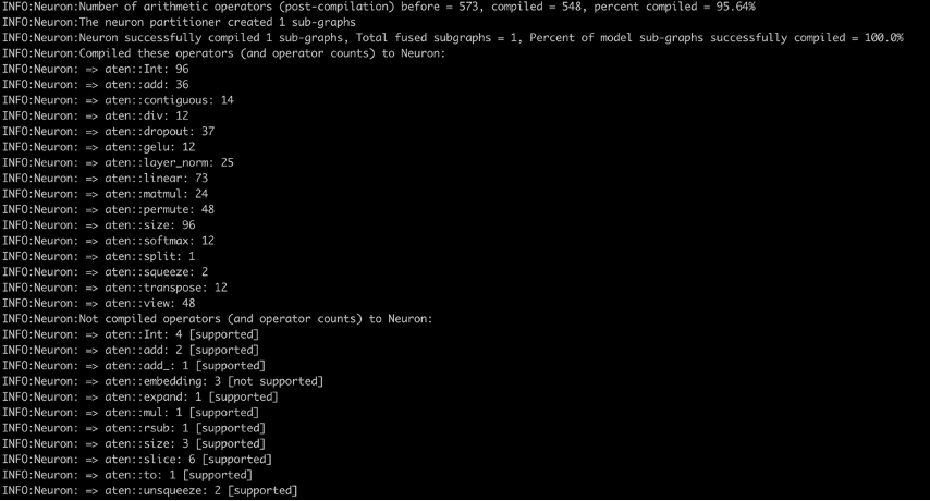
Here is a list of all supported operators in the latest PyTorch Neuron package. Similarly, here is the list of all supported operators in the latest PyTorch Neuronx package.
Deploy models with FastAPI
After the models are compiled, the traced model will be present in the trace-model folder. In this example, we have placed the traced model for a batch size of 1. We consider a batch size of 1 here to account for those use cases where a higher batch size is not feasible or required. For use cases where higher batch sizes are needed, the torch.neuron.DataParallel (for Inf1) or torch.neuronx.DataParallel (for Inf2) API may also be useful.
The fast-api folder provides all the necessary scripts to deploy models with FastAPI. To deploy the models without any changes, simply run the deploy.sh script and it will build a FastAPI container image, run containers on the specified number of cores, and deploy the specified number of models per server in each FastAPI model server. This folder also contains a .env file, modify it to reflect the correct CHIP_TYPE and AWS_DEFAULT_REGION.
Note: FastAPI scripts rely on the same environment variables used to build, push and run the images as containers. FastAPI deployment scripts will use the last known values from these variables. So, if you traced the model for Inf1 instance type last, that model will be deployed through these scripts.
The fastapi-server.py file which is responsible for hosting the server and sending the requests to the model does the following:
- Reads the number of models per server and the location of the compiled model from the properties file
- Sets visible NeuronCores as environment variables to the Docker container and reads the environment variables to specify which NeuronCores to use
- Provides an inference API for the
bert-base-uncased-squad2 model
- With
jit.load(), loads the number of models per server as specified in the config and stores the models and the required tokenizers in global dictionaries
With this setup, it would be relatively easy to set up APIs that list which models and how many models are stored in each NeuronCore. Similarly, APIs could be written to delete models from specific NeuronCores.
The Dockerfile for building FastAPI containers is built on the Docker image we built for tracing the models. This is why the docker.properties file specifies the ECR path to the Docker image for tracing the models. In our setup, the Docker containers across all NeuronCores are similar, so we can build one image and run multiple containers from one image. To avoid any entry point errors, we specify ENTRYPOINT ["/usr/bin/env"] in the Dockerfile before running the startup.sh script, which looks like hypercorn fastapi-server:app -b 0.0.0.0:8080. This startup script is the same for all containers. If you’re using the same base image as for tracing models, you can build this container by simply running the build.sh script. The push.sh script remains the same as before for tracing models. The modified Docker image and container name are provided by the docker.properties file.
The run.sh file does the following:
- Reads the Docker image and container name from the properties file, which in turn reads the
config.properties file, which has a num_cores user setting
- Starts a loop from 0 to
num_cores and for each core:
- Sets the port number and device number
- Sets the
NEURON_RT_VISIBLE_CORES environment variable
- Specifies the volume mount
- Runs a Docker container
For clarity, the Docker run command for deploying in NeuronCore 0 for Inf1 would look like the following code:
docker run -t -d
	    --name $ bert-inf-fastapi-nc-0
	    --env NEURON_RT_VISIBLE_CORES="0-0"
	    --env CHIP_TYPE="inf1"
	    -p ${port_num}:8080 --device=/dev/neuron0 ${registry}/ bert-inf-fastapi
The run command for deploying in NeuronCore 5 would look like the following code:
docker run -t -d
	    --name $ bert-inf-fastapi-nc-5
	    --env NEURON_RT_VISIBLE_CORES="5-5"
	    --env CHIP_TYPE="inf1"
	    -p ${port_num}:8080 --device=/dev/neuron0 ${registry}/ bert-inf-fastapi
After the containers are deployed, we use the run_apis.py script, which calls the APIs in parallel threads. The code is set up to call six models deployed, one on each NeuronCore, but can be easily changed to a different setting. We call the APIs from the client side as follows:
import requests

url_template = http://localhost:%i/predictions_neuron_core_%i/model_%i

# NeuronCore 0
response = requests.get(url_template % (8081,0,0))

# NeuronCore 5
response = requests.get(url_template % (8086,5,0))
Monitor NeuronCore
After the model servers are deployed, to monitor NeuronCore utilization, we may use neuron-top to observe in real time the utilization percentage of each NeuronCore. neuron-top is a CLI tool in the Neuron SDK to provide information such as NeuronCore, vCPU, and memory utilization. In a separate terminal, enter the following command:
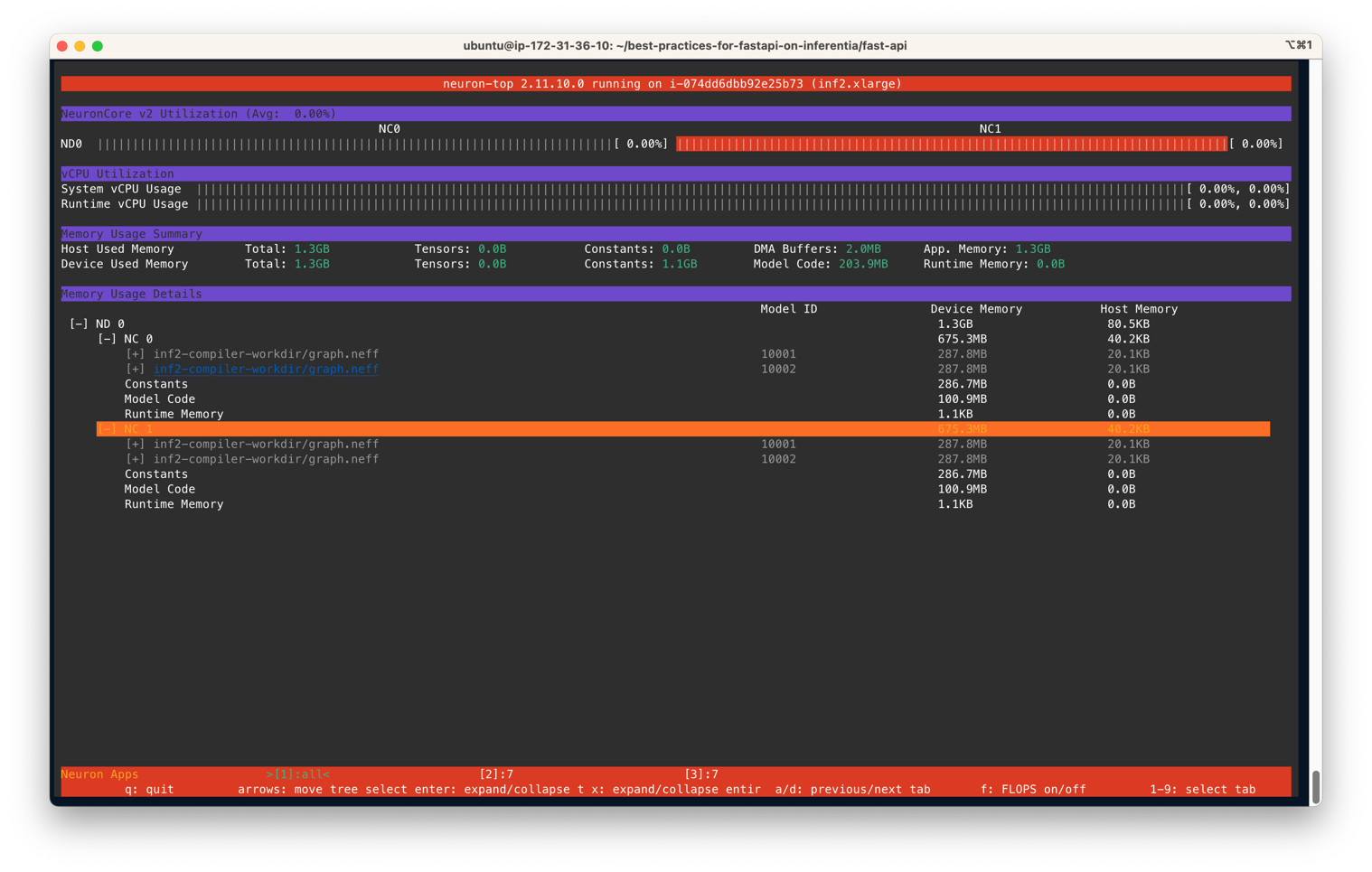
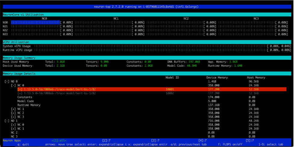
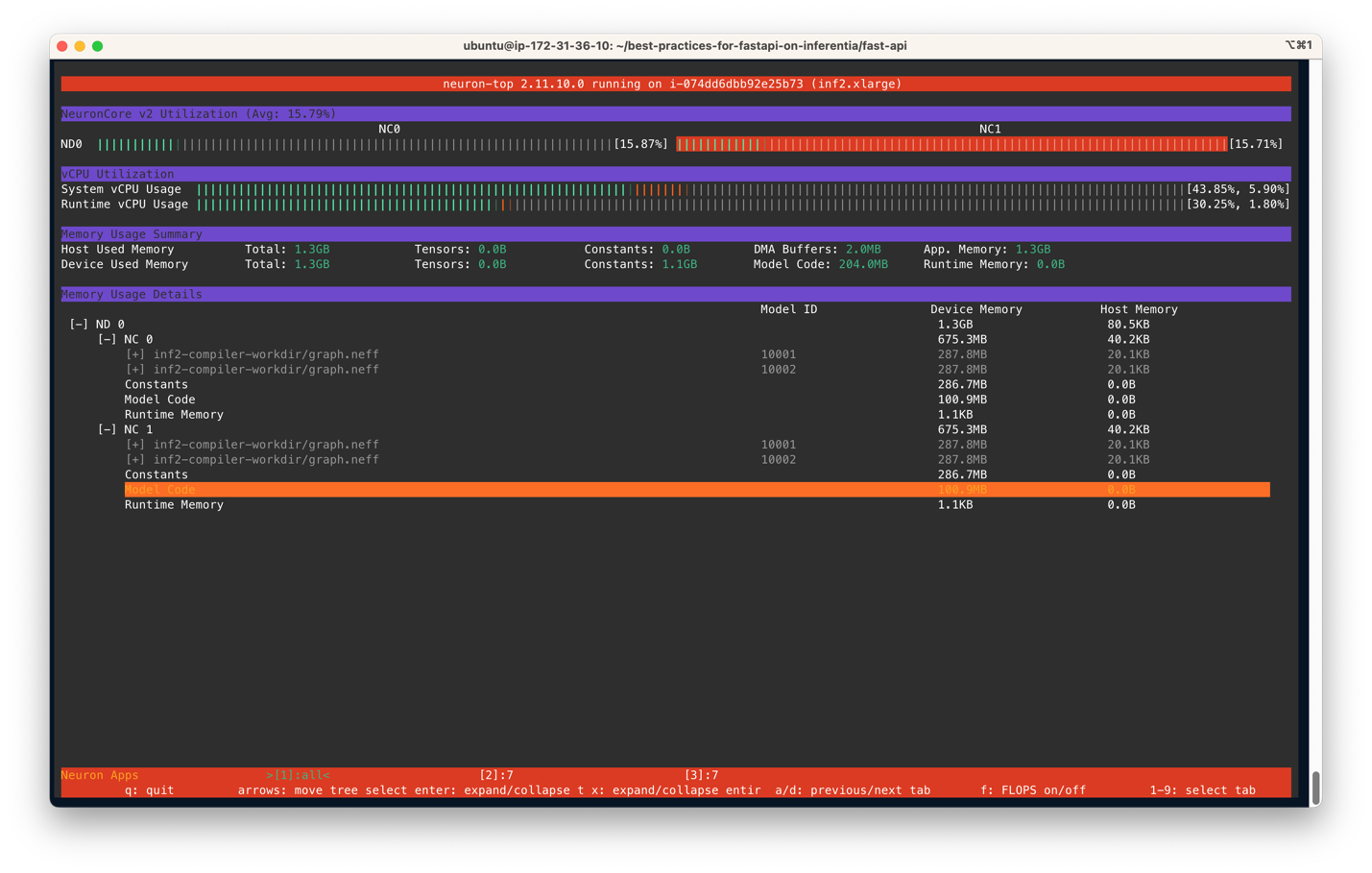
You output should be similar to the following figure. In this scenario, we have specified to use two NeuronCores and two models per server on an Inf2.xlarge instance. The following screenshot shows that two models of size 287.8MB each are loaded on two NeuronCores. With a total of 4 models loaded, you can see the device memory used is 1.3 GB. Use the arrow keys to move between the NeuronCores on different devices
Similarly, on an Inf1.16xlarge instance type we see a total of 12 models (2 models per core over 6 cores) loaded. A total memory of 2.1GB is consumed and every model is 177.2MB in size.
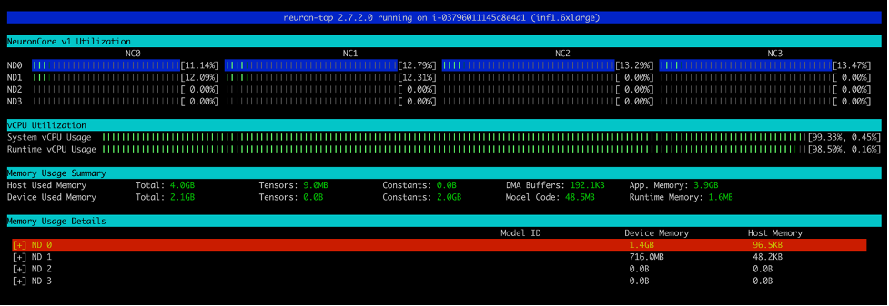
After you run the run_apis.py script, you can see the percentage of utilization of each of the six NeuronCores (see the following screenshot). You can also see the system vCPU usage and runtime vCPU usage.
The following screenshot shows the Inf2 instance core usage percentage.
Similarly, this screenshot shows core utilization in an inf1.6xlarge instance type.
Clean up
To clean up all the Docker containers you created, we provide a cleanup.sh script that removes all running and stopped containers. This script will remove all containers, so don’t use it if you want to keep some containers running.
Conclusion
Production workloads often have high throughput, low latency, and cost requirements. Inefficient architectures that sub-optimally utilize accelerators could lead to unnecessarily high production costs. In this post, we showed how to optimally utilize NeuronCores with FastAPI to maximize throughput at minimum latency. We have published the instructions on our GitHub repo. With this solution architecture, you can deploy multiple models in each NeuronCore and operate multiple models in parallel on different NeuronCores without losing performance. For more information on how to deploy models at scale with services like Amazon Elastic Kubernetes Service (Amazon EKS), refer to Serve 3,000 deep learning models on Amazon EKS with AWS Inferentia for under $50 an hour.
About the authors
 Ankur Srivastava is a Sr. Solutions Architect in the ML Frameworks Team. He focuses on helping customers with self-managed distributed training and inference at scale on AWS. His experience includes industrial predictive maintenance, digital twins, probabilistic design optimization and has completed his doctoral studies from Mechanical Engineering at Rice University and post-doctoral research from Massachusetts Institute of Technology.
 K.C. Tung is a Senior Solution Architect in AWS Annapurna Labs. He specializes in large deep learning model training and deployment at scale in cloud. He has a Ph.D. in molecular biophysics from the University of Texas Southwestern Medical Center in Dallas. He has spoken at AWS Summits and AWS Reinvent. Today he helps customers to train and deploy large PyTorch and TensorFlow models in AWS cloud. He is the author of two books: Learn TensorFlow Enterprise and TensorFlow 2 Pocket Reference.
 Pronoy Chopra is a Senior Solutions Architect with the Startups Generative AI team at AWS. He specializes in architecting and developing IoT and Machine Learning solutions. He has co-founded two startups in the past and enjoys being hands-on with projects in the IoT, AI/ML and Serverless domain.
Read More
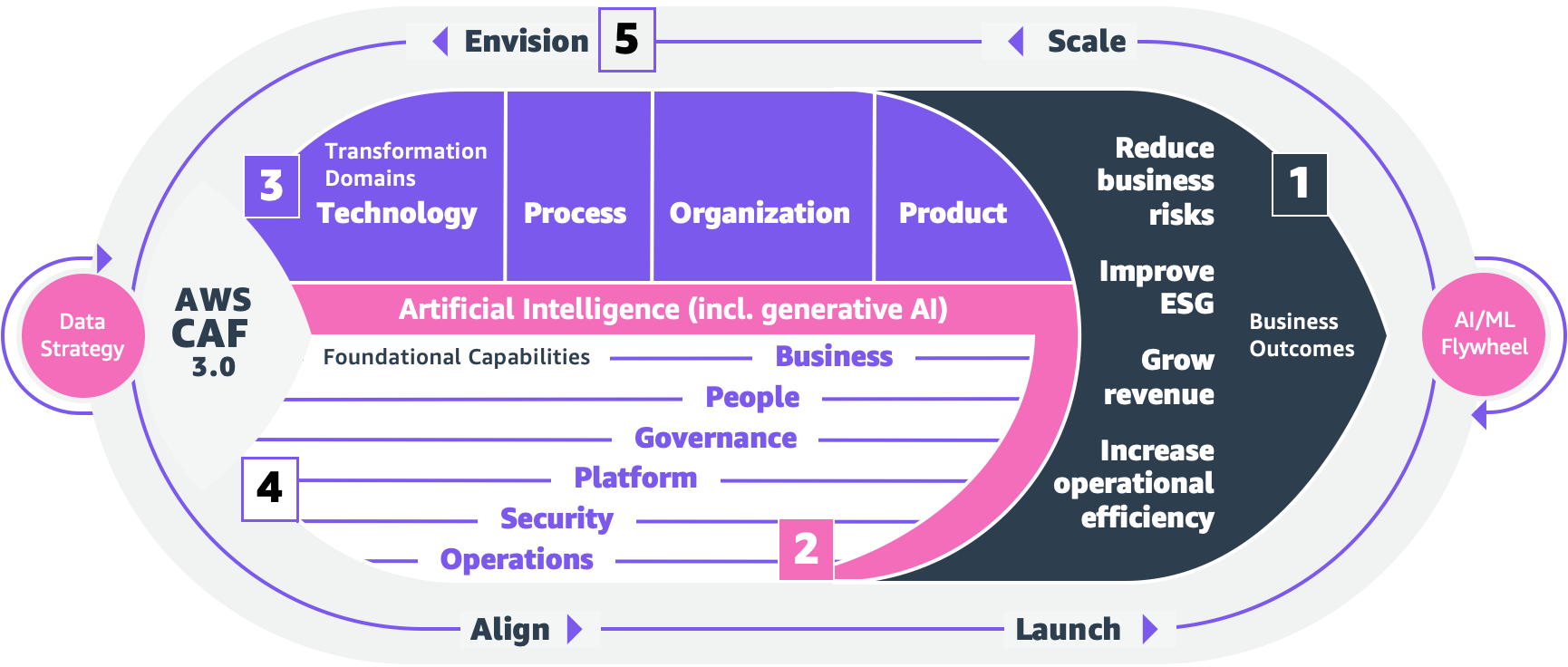
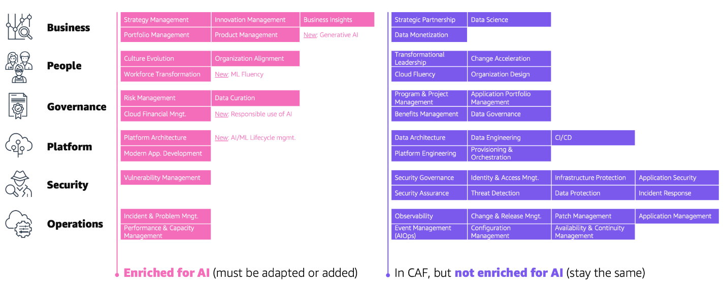

 Caleb Wilkinson has more than a decade of experience building AI solutions. As a Senior Machine Learning Strategist at AWS, Caleb pioneers innovative applications of AI that push the boundaries of possibility and helps organizations benefit responsibly from artificial intelligence. He is the co-author of CAF-AI.
 Alexander Wöhlke has a decade of experience in AI and ML. He is Senior Machine Learning Strategist and Technical Product Manager at the AWS Generative AI Innovation Center. He works with large organizations on their AI-Strategy and helps them take calculated risks at the forefront of technological development. He is the co-author of CAF-AI.
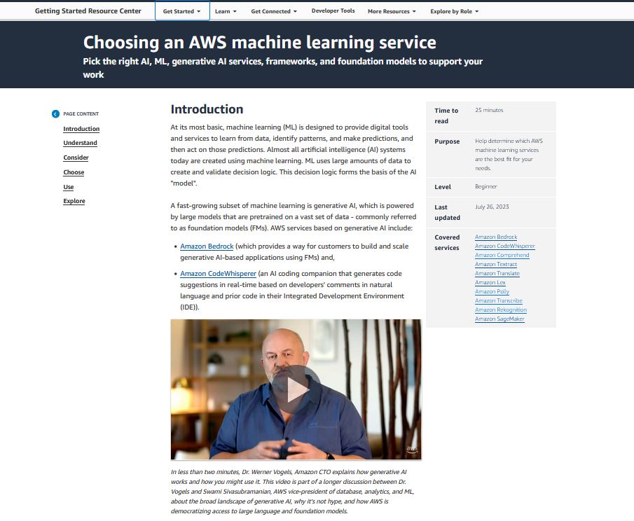
 Geof Wheelwright manages the AWS decision content team, which writes and develops the growing collection of decision guides on the AWS Getting Started Resource Center. His team created the Choosing an AWS machine learning decision guide. He has enjoyed working with AI and its ancestors since first being introduced to simple, text-based Apple II versions of ELIZA in the early 1980s.


 Mehran Nikoo is a Senior Solutions Architect at AWS, working with Digital Native businesses in the UK and helping them achieve their goals. Passionate about applying his software engineering experience to machine learning, he specializes in end-to-end machine learning and MLOps practices.


 Guang Yang is a senior applied scientist at the AWS Generative AI Innovation Center where he works with customers across various verticals and applies creative problem solving to generate value for customers with state-of-the-art ML/AI solutions.
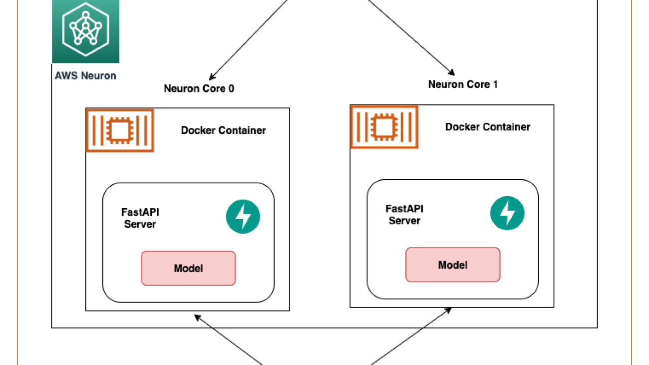


 Bunny Kaushik is a Solutions Architect at AWS. He is passionate about building AI/ML solutions and helping customers innovate on the AWS platform. Outside of work, he enjoys hiking, rock climbing, and swimming.
 Clarisse Vigal is a Sr. Technical Account Manager at AWS, focused on helping customers accelerate their cloud adoption journey. Outside of work, Clarisse enjoys traveling, hiking, and reading sci-fi thrillers.
 Veda Raman is a Senior Specialist Solutions Architect for machine learning based in Maryland. Veda works with customers to help them architect efficient, secure and scalable machine learning applications. Veda is interested in helping customers leverage serverless technologies for Machine learning.