Amazon SageMaker is a fully managed machine learning (ML) platform that offers a comprehensive set of services that serve end-to-end ML workloads. As recommended by AWS as a best practice, customers have used separate accounts to simplify policy management for users and isolate resources by workloads and account. However, when more users and teams are using the ML platform in the cloud, monitoring the large ML workloads in a scaling multi-account environment becomes more challenging. For better observability, customers are looking for solutions to monitor the cross-account resource usage and track activities, such as job launch and running status, which is essential for their ML governance and management requirements.
SageMaker services, such as Processing, Training, and Hosting, collect metrics and logs from the running instances and push them to users’ Amazon CloudWatch accounts. To view the details of these jobs in different accounts, you need to log in to each account, find the corresponding jobs, and look into the status. There is no single pane of glass that can easily show this cross-account and multi-job information. Furthermore, the cloud admin team needs to provide individuals access to different SageMaker workload accounts, which adds additional management overhead for the cloud platform team.
In this post, we present a cross-account observability dashboard that provides a centralized view for monitoring SageMaker user activities and resources across multiple accounts. It allows the end-users and cloud management team to efficiently monitor what ML workloads are running, view the status of these workloads, and trace back different account activities at certain points of time. With this dashboard, you don’t need to navigate from the SageMaker console and click into each job to find the details of the job logs. Instead, you can easily view the running jobs and job status, troubleshoot job issues, and set up alerts when issues are identified in shared accounts, such as job failure, underutilized resources, and more. You can also control access to this centralized monitoring dashboard or share the dashboard with relevant authorities for auditing and management requirements.
Overview of solution
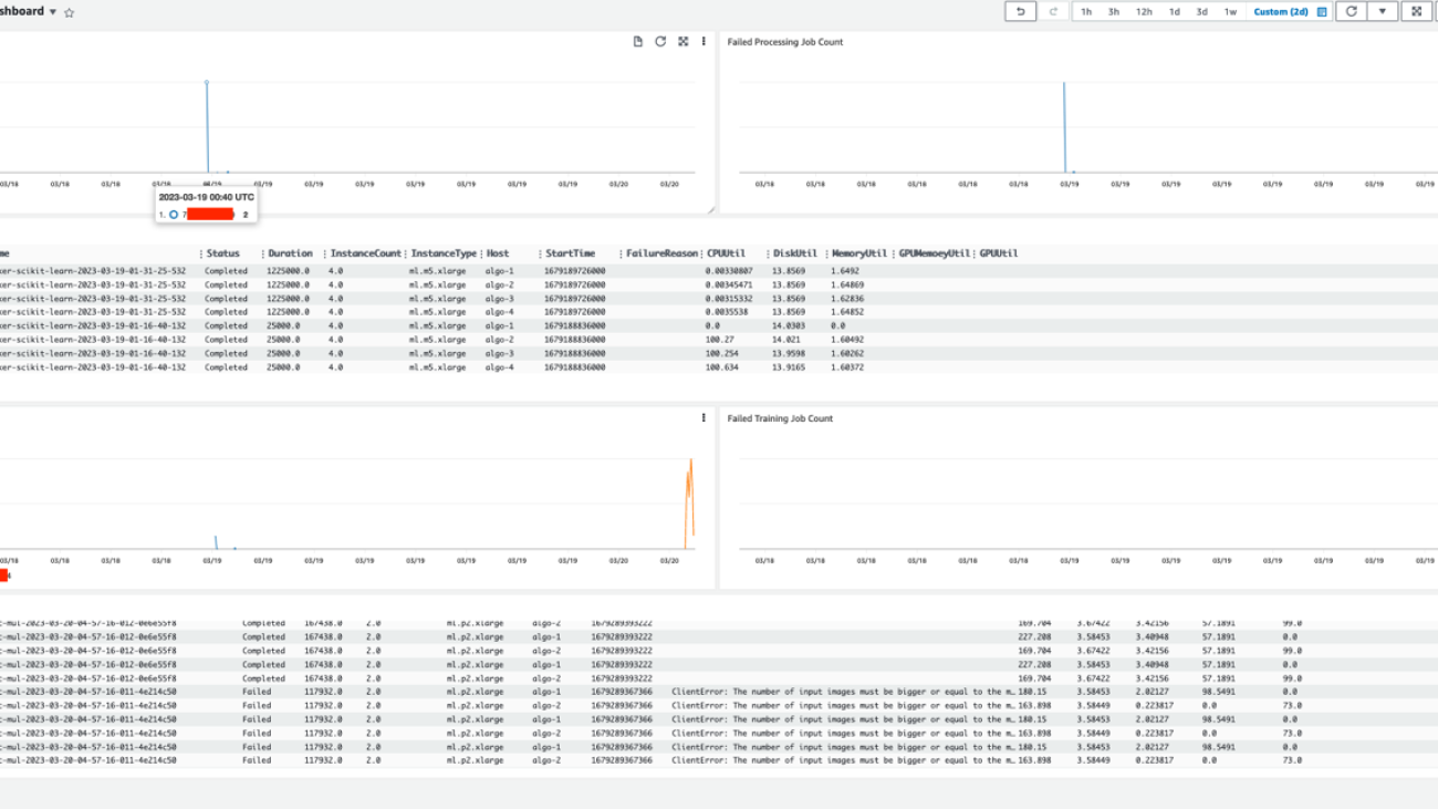
This solution is designed to enable centralized monitoring of SageMaker jobs and activities across a multi-account environment. The solution is designed to have no dependency on AWS Organizations, but can be adopted easily in an Organizations or AWS Control Tower environment. This solution can help the operation team have a high-level view of all SageMaker workloads spread across multiple workload accounts from a single pane of glass. It also has an option to enable CloudWatch cross-account observability across SageMaker workload accounts to provide access to monitoring telemetries such as metrics, logs, and traces from the centralized monitoring account. An example dashboard is shown in the following screenshot.

The following diagram shows the architecture of this centralized dashboard solution.

SageMaker has native integration with the Amazon EventBridge, which monitors status change events in SageMaker. EventBridge enables you to automate SageMaker and respond automatically to events such as a training job status change or endpoint status change. Events from SageMaker are delivered to EventBridge in near-real time. For more information about SageMaker events monitored by EventBridge, refer to Automating Amazon SageMaker with Amazon EventBridge. In addition to the SageMaker native events, AWS CloudTrail publishes events when you make API calls, which also streams to EventBridge so that this can be utilized by many downstream automation or monitoring use cases. In our solution, we use EventBridge rules in the workload accounts to stream SageMaker service events and API events to the monitoring account’s event bus for centralized monitoring.
In the centralized monitoring account, the events are captured by an EventBridge rule and further processed into different targets:
- A CloudWatch log group, to use for the following:
- Auditing and archive purposes. For more information, refer to the Amazon CloudWatch Logs User Guide.
- Analyzing log data with CloudWatch Log Insights queries. CloudWatch Logs Insights enables you to interactively search and analyze your log data in CloudWatch Logs. You can perform queries to help you more efficiently and effectively respond to operational issues. If an issue occurs, you can use CloudWatch Logs Insights to identify potential causes and validate deployed fixes.
- Support for the CloudWatch Metrics Insights query widget for high-level operations in the CloudWatch dashboard, adding CloudWatch Insights Query to dashboards, and exporting query results.
- An AWS Lambda function to complete the following tasks:
- Perform custom logic to augment SageMaker service events. One example is performing a metric query on the SageMaker job host’s utilization metrics when a job completion event is received.
- Convert event information into metrics in certain log formats as ingested as EMF logs. For more information, refer to Embedding metrics within logs.
The example in this post is supported by the native CloudWatch cross-account observability feature to achieve cross-account metrics, logs, and trace access. As shown at the bottom of the architecture diagram, it integrates with this feature to enable cross-account metrics and logs. To enable this, necessary permissions and resources need to be created in both the monitoring accounts and source workload accounts.
You can use this solution for either AWS accounts managed by Organizations or standalone accounts. The following sections explain the steps for each scenario. Note that within each scenario, steps are performed in different AWS accounts. For your convenience, the account type to perform the step is highlighted at the beginning each step.
Prerequisites
Before starting this procedure, clone our source code from the GitHub repo in your local environment or AWS Cloud9. Additionally, you need the following:
- Node.js 14.15.0 (or later) and nmp installed
- The AWS Command Line Interface (AWS CLI) version 2 installed
- The AWS CDK Toolkit
- Docker Engine installed (in running state when performing the deployment procedures)

Deploy the solution in an Organizations environment
If the monitoring account and all SageMaker workload accounts are all in the same organization, the required infrastructure in the source workload accounts is created automatically via an AWS CloudFormation StackSet from the organization’s management account. Therefore, no manual infrastructure deployment into the source workload accounts is required. When a new account is created or an existing account is moved into a target organizational unit (OU), the source workload infrastructure stack will be automatically deployed and included in the scope of centralized monitoring.
Set up monitoring account resources
We need to collect the following AWS account information to set up the monitoring account resources, which we use as the inputs for the setup script later on.
| Input | Description | Example |
| Home Region | The Region where the workloads run. | ap-southeast-2 |
| Monitoring account AWS CLI profile name | You can find the profile name from ~/.aws/config. This is optional. If not provided, it uses the default AWS credentials from the chain. |
. |
| SageMaker workload OU path | The OU path that has the SageMaker workload accounts. Keep the / at the end of the path. |
o-1a2b3c4d5e/r-saaa/ou-saaa-1a2b3c4d/ |
To retrieve the OU path, you can go to the Organizations console, and under AWS accounts, find the information to construct the OU path. For the following example, the corresponding OU path is o-ye3wn3kyh6/r-taql/ou-taql-wu7296by/.

After you retrieve this information, run the following command to deploy the required resources on the monitoring account:
You can get the following outputs from the deployment. Keep a note of the outputs to use in the next step when deploying the management account stack.

Set up management account resources
We need to collect the following AWS account information to set up the management account resources, which we use as the inputs for the setup script later on.
| Input | Description | Example |
| Home Region | The Region where the workloads run. This should be the same as the monitoring stack. | ap-southeast-2 |
| Management account AWS CLI profile name | You can find the profile name from ~/.aws/config. This is optional. If not provided, it uses the default AWS credentials from the chain. |
. |
| SageMaker workload OU ID | Here we use just the OU ID, not the path. | ou-saaa-1a2b3c4d |
| Monitoring account ID | The account ID where the monitoring stack is deployed to. | . |
| Monitoring account role name | The output for MonitoringAccountRoleName from the previous step. |
. |
| Monitoring account event bus ARN | The output for MonitoringAccountEventbusARN from the previous step. |
. |
| Monitoring account sink identifier | The output from MonitoringAccountSinkIdentifier from the previous step. |
. |
You can deploy the management account resources by running the following command:
Deploy the solution in a non-Organizations environment
If your environment doesn’t use Organizations, the monitoring account infrastructure stack is deployed in a similar manner but with a few changes. However, the workload infrastructure stack needs to be deployed manually into each workload account. Therefore, this method is suitable for an environment with a limited number of accounts. For a large environment, it’s recommended to consider using Organizations.
Set up monitoring account resources
We need to collect the following AWS account information to set up the monitoring account resources, which we use as the inputs for the setup script later on.
| Input | Description | Example |
| Home Region | The Region where the workloads run. | ap-southeast-2 |
| SageMaker workload account list | A list of accounts that run the SageMaker workload and stream events to the monitoring account, separated by commas. | 111111111111,222222222222 |
| Monitoring account AWS CLI profile name | You can find the profile name from ~/.aws/config. This is optional. If not provided, it uses the default AWS credentials from the chain. |
. |
We can deploy the monitoring account resources by running the following command after you collect the necessary information:
We get the following outputs when the deployment is complete. Keep a note of the outputs to use in the next step when deploying the management account stack.
Set up workload account monitoring infrastructure
We need to collect the following AWS account information to set up the workload account monitoring infrastructure, which we use as the inputs for the setup script later on.
| Input | Description | Example |
| Home Region | The Region where the workloads run. This should be the same as the monitoring stack. | ap-southeast-2 |
| Monitoring account ID | The account ID where the monitoring stack is deployed to. | . |
| Monitoring account role name | The output for MonitoringAccountRoleName from the previous step. |
. |
| Monitoring account event bus ARN | The output for MonitoringAccountEventbusARN from the previous step. |
. |
| Monitoring account sink identifier | The output from MonitoringAccountSinkIdentifier from the previous step. |
. |
| Workload account AWS CLI profile name | You can find the profile name from ~/.aws/config. This is optional. If not provided, it uses the default AWS credentials from the chain. |
. |
We can deploy the monitoring account resources by running the following command:
Visualize ML tasks on the CloudWatch dashboard
To check if the solution works, we need to run multiple SageMaker processing jobs and SageMaker training jobs on the workload accounts that we used in the previous sections. The CloudWatch dashboard is customizable based on your own scenarios. Our sample dashboard consists of widgets for visualizing SageMaker Processing jobs and SageMaker Training jobs. All jobs for monitoring workload accounts are displayed in this dashboard. In each type of job, we show three widgets, which are the total number of jobs, the number of failing jobs, and the details of each job. In our example, we have two workload accounts. Through this dashboard, we can easily find that one workload account has both processing jobs and training jobs, and another workload account only has training jobs. As with the functions we use in CloudWatch, we can set the refresh interval, specify the graph type, and zoom in or out, or we can run actions such as download logs in a CSV file.
Customize your dashboard
The solution provided in the GitHub repo includes both SageMaker Training job and SageMaker Processing job monitoring. If you want to add more dashboards to monitor other SageMaker jobs, such as batch transform jobs, you can follow the instructions in this section to customize your dashboard. By modifying the index.py file, you can customize the fields what you want to display on the dashboard. You can access all details that are captured by CloudWatch through EventBridge. In the Lambda function, you can choose the necessary fields that you want to display on the dashboard. See the following code:
To customize the dashboard or widgets, you can modify the source code in the monitoring-account-infra-stack.ts file. Note that the field names you use in this file should be the same as those (the keys of job_detail) defined in the Lambda file:
After you modify the dashboard, you need to redeploy this solution from scratch. You can run the Jupyter notebook provided in the GitHub repo to rerun the SageMaker pipeline, which will launch the SageMaker Processing jobs again. When the jobs are finished, you can go to the CloudWatch console, and under Dashboards in the navigation pane, choose Custom Dashboards. You can find the dashboard named SageMaker-Monitoring-Dashboard.
Clean up
If you no longer need this custom dashboard, you can clean up the resources. To delete all the resources created, use the code in this section. The cleanup is slightly different for an Organizations environment vs. a non-Organizations environment.
For an Organizations environment, use the following code:
For a non-Organizations environment, use the following code:
Alternatively, you can log in to the monitoring account, workload account, and management account to delete the stacks from the CloudFormation console.
Conclusion
In this post, we discussed the implementation of a centralized monitoring and reporting solution for SageMaker using CloudWatch. By following the step-by-step instructions outlined in this post, you can create a multi-account monitoring dashboard that displays key metrics and consolidates logs related to their various SageMaker jobs from different accounts in real time. With this centralized monitoring dashboard, you can have better visibility into the activities of SageMaker jobs across multiple accounts, troubleshoot issues more quickly, and make informed decisions based on real-time data. Overall, the implementation of a centralized monitoring and reporting solution using CloudWatch offers an efficient way for organizations to manage their cloud-based ML infrastructure and resource utilization.
Please try out the solution and send us the feedback, either in the AWS forum for Amazon SageMaker, or through your usual AWS contacts.
To learn more about the cross-account observability feature, please refer to the blog Amazon CloudWatch Cross-Account Observability
About the Authors
 Jie Dong is an AWS Cloud Architect based in Sydney, Australia. Jie is passionate about automation, and loves to develop solutions to help customer improve productivity. Event-driven system and serverless framework are his expertise. In his own time, Jie loves to work on building smart home and explore new smart home gadgets.
 Melanie Li, PhD, is a Senior AI/ML Specialist TAM at AWS based in Sydney, Australia. She helps enterprise customers build solutions using state-of-the-art AI/ML tools on AWS and provides guidance on architecting and implementing ML solutions with best practices. In her spare time, she loves to explore nature and spend time with family and friends.
 Gordon Wang, is a Senior AI/ML Specialist TAM at AWS. He supports strategic customers with AI/ML best practices cross many industries. He is passionate about computer vision, NLP, Generative AI and MLOps. In his spare time, he loves running and hiking.


 Fabian Benitez-Quiroz is a IoT Edge Data Scientist in AWS Professional Services. He holds a PhD in Computer Vision and Pattern Recognition from The Ohio State University. Fabian is involved in helping customers run their machine learning models with low latency on IoT devices and in the cloud across various industries.
 Romil Shah is a Sr. Data Scientist at AWS Professional Services. Romil has more than 6 years of industry experience in computer vision, machine learning, and IoT edge devices. He is involved in helping customers optimize and deploy their machine learning models for edge devices and on the cloud. He works with customers to create strategies for optimizing and deploying foundation models.
 Han Man is a Senior Data Science & Machine Learning Manager with AWS Professional Services based in San Diego, CA. He has a PhD in Engineering from Northwestern University and has several years of experience as a management consultant advising clients in manufacturing, financial services, and energy. Today, he is passionately working with key customers from a variety of industry verticals to develop and implement ML and GenAI solutions on AWS.


 Giuseppe Angelo Porcelli is a Principal Machine Learning Specialist Solutions Architect for Amazon Web Services. With several years software engineering and an ML background, he works with customers of any size to understand their business and technical needs and design AI and ML solutions that make the best use of the AWS Cloud and the Amazon Machine Learning stack. He has worked on projects in different domains, including MLOps, computer vision, and NLP, involving a broad set of AWS services. In his free time, Giuseppe enjoys playing football.
 Bruno Pistone is an AI/ML Specialist Solutions Architect for AWS based in Milan. He works with customers of any size, helping them understand their technical needs and design AI and ML solutions that make the best use of the AWS Cloud and the Amazon Machine Learning stack. His field of expertice includes machine learning end to end, machine learning endustrialization, and generative AI. He enjoys spending time with his friends and exploring new places, as well as traveling to new destinations.
 Saurabh Trikande is a Senior Product Manager for Amazon SageMaker Inference. He is passionate about working with customers and is motivated by the goal of democratizing machine learning. He focuses on core challenges related to deploying complex ML applications, multi-tenant ML models, cost optimizations, and making deployment of deep learning models more accessible. In his spare time, Saurabh enjoys hiking, learning about innovative technologies, following TechCrunch, and spending time with his family.
 Nikhil Kulkarni is a software developer with AWS Machine Learning, focusing on making machine learning workloads more performant on the cloud, and is a co-creator of AWS Deep Learning Containers for training and inference. He’s passionate about distributed Deep Learning Systems. Outside of work, he enjoys reading books, fiddling with the guitar, and making pizza.
 Uri Rosenberg is the AI & ML Specialist Technical Manager for Europe, Middle East, and Africa. Based out of Israel, Uri works to empower enterprise customers to design, build, and operate ML workloads at scale. In his spare time, he enjoys cycling, backpacking, and backpropagating.
 Eliuth Triana Isaza is a Developer Relations Manager on the NVIDIA-AWS team. He connects Amazon and AWS product leaders, developers, and scientists with NVIDIA technologists and product leaders to accelerate Amazon ML/DL workloads, EC2 products, and AWS AI services. In addition, Eliuth is a passionate mountain biker, skier, and poker player.
 James Poquiz is a Data Scientist with AWS Professional Services based in Orange County, California. He has a BS in Computer Science from the University of California, Irvine and has several years of experience working in the data domain having played many different roles. Today he works on implementing and deploying scalable ML solutions to achieve business outcomes for AWS clients.
 Han Man is a Senior Data Science & Machine Learning Manager with AWS Professional Services based in San Diego, CA. He has a PhD in Engineering from Northwestern University and has several years of experience as a management consultant advising clients in manufacturing, financial services, and energy. Today, he is passionately working with key customers from a variety of industry verticals to develop and implement ML and GenAI solutions on AWS.
 Safa Tinaztepe is a full-stack data scientist with AWS Professional Services. He has a BS in computer science from Emory University and has interests in MLOps, distributed systems, and web3.


 Munish Dabra is a Principal Solutions Architect at Amazon Web Services (AWS). His current areas of focus are AI/ML and Observability. He has a strong background in designing and building scalable distributed systems. He enjoys helping customers innovate and transform their business in AWS. LinkedIn:
  Patrick Lin is a Software Development Engineer with Amazon SageMaker Data Wrangler. He is committed to making Amazon SageMaker Data Wrangler the number one data preparation tool for productionized ML workflows. Outside of work, you can find him reading, listening to music, having conversations with friends, and serving at his church.


 Arun Anand is a Senior Solutions Architect at Amazon Web Services based in Houston area. He has 25+ years of experience in designing and developing enterprise applications. He works with partners in Energy & Utilities segment providing architectural and best practice recommendations for new and existing solutions.
 Rajnish Shaw is a Senior Solutions Architect at Amazon Web Services, with a background as a Product Developer and Architect. Rajnish is passionate about helping customers build applications on the cloud. Outside of work Rajnish enjoys spending time with family and friends, and traveling.
 Yuanhua Wang is a software engineer at AWS with more than 15 years of experience in the technology industry. His interests are software architecture and build tools on cloud computing.