This post is co-authored by Daryl Martis, Director of Product, Salesforce Einstein AI.
This is the second post in a series discussing the integration of Salesforce Data Cloud and Amazon SageMaker. In Part 1, we show how the Salesforce Data Cloud and Einstein Studio integration with SageMaker allows businesses to access their Salesforce data securely using SageMaker and use its tools to build, train, and deploy models to endpoints hosted on SageMaker. The endpoints are then registered to the Salesforce Data Cloud to activate predictions in Salesforce.
In this post, we expand on this topic to demonstrate how to use Einstein Studio for product recommendations. You can use this integration for traditional models as well as large language models (LLMs).
Solution overview
In this post, we demonstrate how to create a predictive model in SageMaker to recommend the next best product to your customers by using historical data such as customer demographics, marketing engagements, and purchase history from Salesforce Data Cloud.
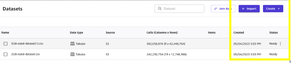
We use the following sample dataset. To use this dataset in your Data Cloud, refer to Create Amazon S3 Data Stream in Data Cloud.
The following attributes are needed to create the model:
- Club Member – If the customer is a club member
- Campaign – The campaign the customer is a part of
- State – The state or province the customer resides in
- Month – The month of purchase
- Case Count – The number of cases raised by the customer
- Case Type Return – Whether the customer returned any product within the last year
- Case Type Shipment Damaged – Whether the customer had any shipments damaged in the last year
- Engagement Score – The level of engagement the customer has (response to mailing campaigns, logins to the online store, and so on)
- Tenure – The tenure of the customer relationship with the company
- Clicks – The average number of clicks the customer has made within a week prior to purchase
- Pages Visited – The average number of pages the customer has visited within a week prior to purchase
- Product Purchased – The actual product purchased
- Id – The ID of the record
- DateTime – The timestamp of the dataset
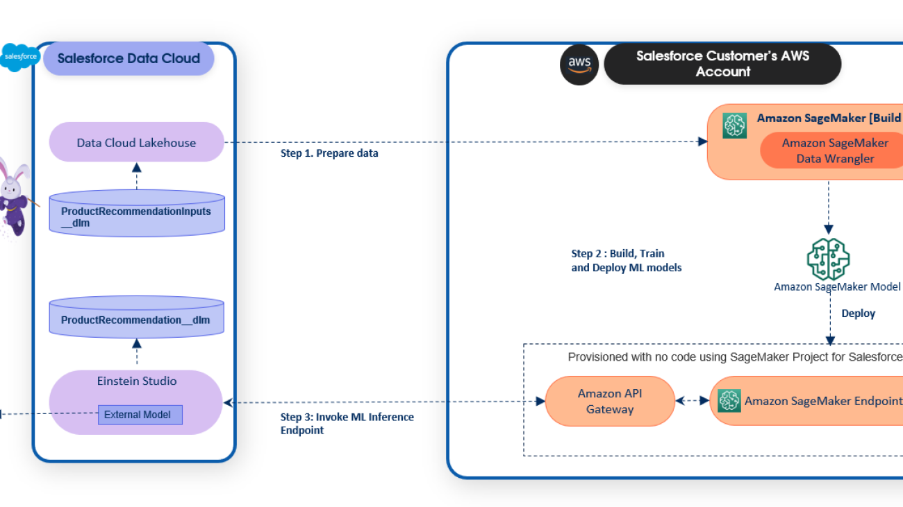
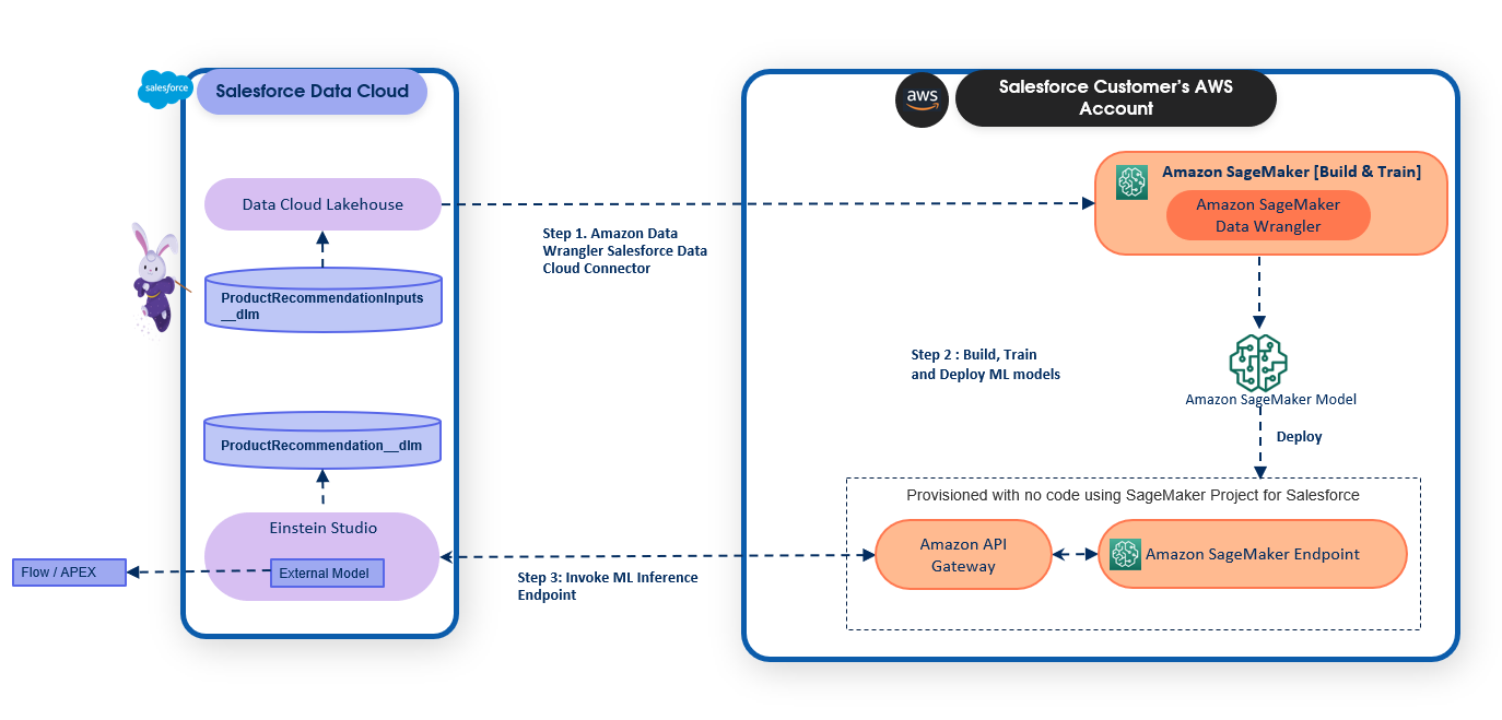
The product recommendation model is built and deployed on SageMaker and is trained using data in the Salesforce Data Cloud. The following steps give an overview of how to use the new capabilities launched in SageMaker for Salesforce to enable the overall integration:
- Set up the Amazon SageMaker Studio domain and OAuth between Salesforce and the AWS account
s. - Use the newly launched capability of the Amazon SageMaker Data Wrangler connector for Salesforce Data Cloud to prepare the data in SageMaker without copying the data from Salesforce Data Cloud.
- Train a recommendation model in SageMaker Studio using training data that was prepared using SageMaker Data Wrangler.
- Package the SageMaker Data Wrangler container and the trained recommendation model container in an inference pipeline so the inference request can use the same data preparation steps you created to preprocess the training data. The real-time inference call data is first passed to the SageMaker Data Wrangler container in the inference pipeline, where it is preprocessed and passed to the trained model for product recommendation. For more information about this process, refer to New — Introducing Support for Real-Time and Batch Inference in Amazon SageMaker Data Wrangler. Although we use a specific algorithm to train the model in our example, you can use any algorithm that you find appropriate for your use case.
- Use the newly launched SageMaker provided project template for Salesforce Data Cloud integration to streamline implementing the preceding steps by providing the following templates:
- An example notebook showcasing data preparation, building, training, and registering the model.
- The SageMaker provided project template for Salesforce Data Cloud integration, which automates creating a SageMaker endpoint hosting the inference pipeline model. When a version of the model in the Amazon SageMaker Model Registry is approved, the endpoint is exposed as an API with Amazon API Gateway using a custom Salesforce JSON Web Token (JWT) authorizer. API Gateway is required to allow Salesforce Data Cloud to make predictions against the SageMaker endpoint using a JWT token that Salesforce creates and passes with the request when making predictions from Salesforce. JWT can be used as a part of OpenID Connect (OIDC) and OAuth 2.0 frameworks to restrict client access to your APIs.
- After you create the API, we recommend registering the model endpoint in Salesforce Einstein Studio. For instructions, refer to Bring Your Own AI Models to Salesforce with Einstein Studio
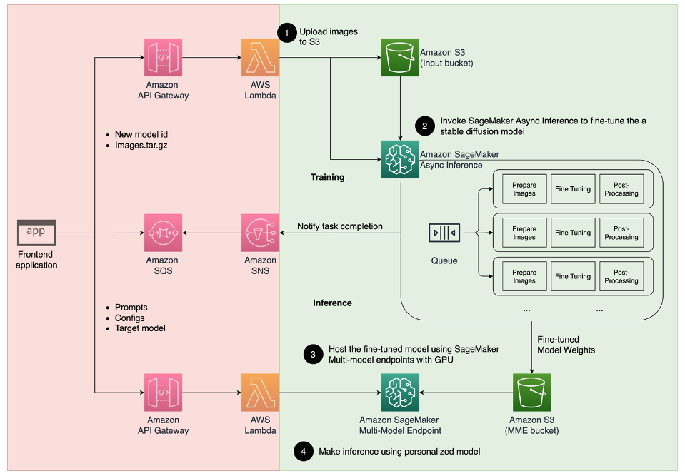
The following diagram illustrates the solution architecture.

Create a SageMaker Studio domain
First, create a SageMaker Studio domain. For instructions, refer to Onboard to Amazon SageMaker Domain. You should note down the domain ID and execution role that is created and will be used by your user profile. You add permissions to this role in subsequent steps.
The following screenshot shows the domain we created for this post.

The following screenshot shows the example user profile for this post.

Set up the Salesforce connected app
Next, we create a Salesforce connected app to enable the OAuth flow from SageMaker Studio to Salesforce Data Cloud. Complete the following steps:
- Log in to Salesforce and navigate to Setup.
- Search for App Manager and create a new connected app.
- Provide the following inputs:
- For Connected App Name, enter a name.
- For API Name, leave as default (it’s automatically populated).
- For Contact Email, enter your contact email address.
- Select Enable OAuth Settings.
- For Callback URL, enter
https://<domain-id>.studio.<region>.sagemaker.aws/jupyter/default/lab, and provide the domain ID that you captured while creating the SageMaker domain and the Region of your SageMaker domain.
- Under Selected OAuth Scopes, move the following from Available OAuth Scopes to Selected OAuth Scopes and choose Save:
- Manage user data via APIs (api)
- Perform requests at any time (
refresh_token,offline_access) - Perform ANSI SQL queries on Salesforce Data Cloud data (Data Cloud_query_api)
- Manage Salesforce Customer Data Platform profile data (Data Cloud_profile_api
- Access the identity URL service (id, profile, email, address, phone)
- Access unique user identifiers (
openid)
For more information about creating a connected app, refer to Create a Connected App.

- Return to the connected app and navigate to Consumer Key and Secret.
- Choose Manage Consumer Details.

- Copy the key and secret.
You may be asked to log in to your Salesforce org as part of the two-factor authentication here.

- Navigate back to the Manage Connected Apps page.
- Open the connected app you created and choose Manage.
- Choose Edit Policies and change IP Relaxation to Relax IP restrictions, then save your settings.
Configure SageMaker permissions and lifecycle rules
In this section, we walk through the steps to configure SageMaker permissions and lifecycle management rules.
Create a secret in AWS Secrets Manager
Enable OAuth integration with Salesforce Data Cloud by storing credentials from your Salesforce connected app in AWS Secrets Manager:
- On the Secrets Manager console, choose Store a new secret.
- Select Other type of secret.
- Create your secret with the following key-value pairs:
- Add a tag with the key
sagemaker:partnerand your choice of value. - Save the secret and note the ARN of the secret.

Configure a SageMaker lifecycle rule
The SageMaker Studio domain execution role will require AWS Identity and Access Management (IAM) permissions to access the secret created in the previous step. For more information, refer to Creating roles and attaching policies (console).
- On the IAM console, attach the following polices to their respective roles (these roles will be used by the SageMaker project for deployment):
- Add the policy
AmazonSageMakerPartnerServiceCatalogProductsCloudFormationServiceRolePolicyto the service roleAmazonSageMakerServiceCatalogProductsCloudformationRole. - Add the policy
AmazonSageMakerPartnerServiceCatalogProductsApiGatewayServiceRolePolicyto the service roleAmazonSageMakerServiceCatalogProductsApiGatewayRole. - Add the policy
AmazonSageMakerPartnerServiceCatalogProductsLambdaServiceRolePolicyto the service roleAmazonSageMakerServiceCatalogProductsLambdaRole.
- Add the policy
- On the IAM console, navigate to the SageMaker domain execution role.
- Choose Add permissions and select Create an inline policy.
- Enter the following policy in the JSON policy editor:
SageMaker Studio lifecycle configuration provides shell scripts that run when a notebook is created or started. The lifecycle configuration will be used to retrieve the secret and import it to the SageMaker runtime.
- On the SageMaker console, choose Lifecycle configurations in the navigation pane.
- Choose Create configuration.
- Leave the default selection Jupyter Server App and choose Next.
- Give the configuration a name.
- Enter the following script in the editor, providing the ARN for the secret you created earlier:

- Choose Submit to save the lifecycle configuration.
- Choose Domains in the navigation pane and open your domain.
- On the Environment tab, choose Attach to attach your lifecycle configuration.
- Choose the lifecycle configuration you created and choose Attach to domain.
- Choose Set as default.
If you are a returning user to SageMaker Studio, in order to ensure Salesforce Data Cloud is enabled, upgrade to the latest Jupyter and SageMaker Data Wrangler kernels.
This completes the setup to enable data access from Salesforce Data Cloud to SageMaker Studio to build AI and machine learning (ML) models.
Create a SageMaker project
To start using the solution, first create a project using Amazon SageMaker Projects. Complete the following steps:
- In SageMaker Studio, under Deployments in the navigation pane, choose Projects.
- Choose Create project.
- Choose the project template called Model deployment for Salesforce.
- Choose Select project template.

- Enter a name and optional description for your project.
- Enter a model group name.
- Enter the name of the Secrets Manager secret that you created earlier.
- Choose Create project.
The project may take 1–2 minutes to initiate.

You can see two new repositories. The first one is for sample notebooks that you can use as is or customize to prepare, train, create, and register models in the SageMaker Model Registry. The second repository is for automating the model deployment, which includes exposing the SageMaker endpoint as an API.
- Choose clone repo for both notebooks.

For this post, we use the product recommendation example, which can be found in the sagemaker-<YOUR-PROJECT-NAME>-p-<YOUR-PROJECT-ID>-example-nb/product-recommendation directory that you just cloned. Before we run the product-recommendation.ipynb notebook, let’s do some data preparation to create the training data using SageMaker Data Wrangler.

Prepare data with SageMaker Data Wrangler
Complete the following steps:
- In SageMaker Studio, on the File menu, choose New and Data Wrangler flow.

- After you create the data flow, choose (right-click) the tab and choose Rename to rename the file.
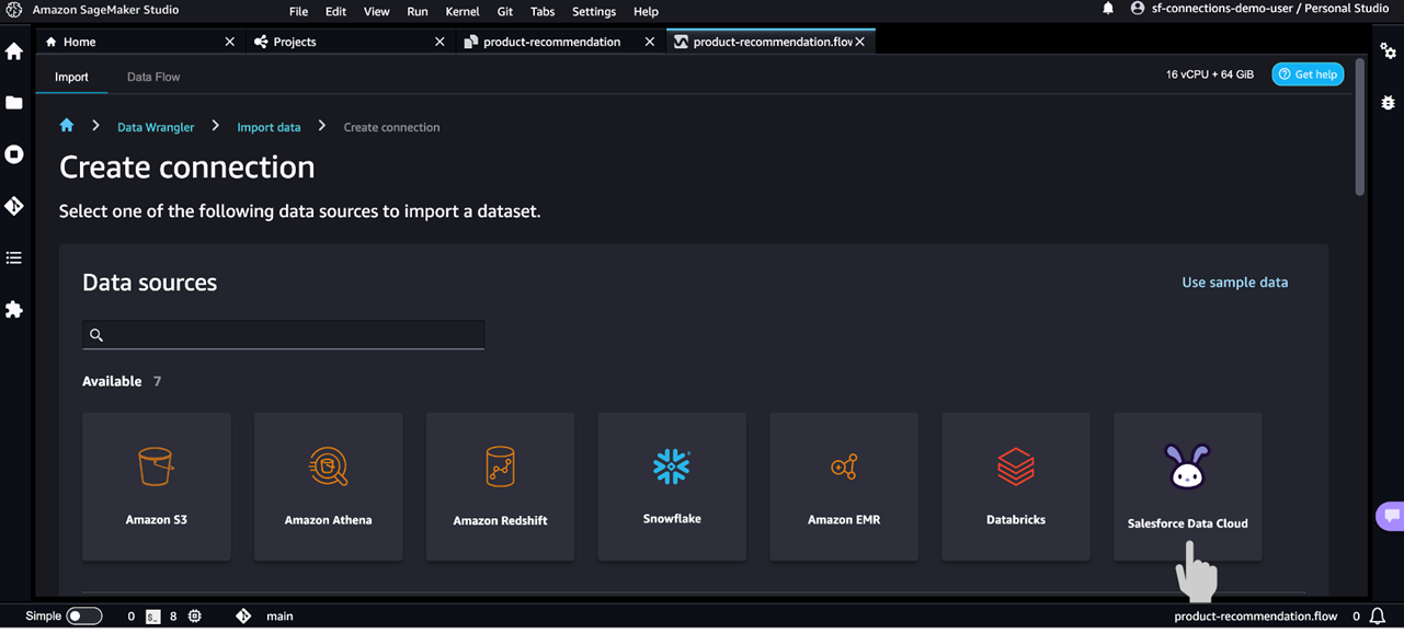
- Choose Import data.

- Choose Create connection.

- Choose Salesforce Data Cloud.

- For Name, enter
salesforce-data-cloud-sagemaker-connection. - For Salesforce org URL, enter your Salesforce org URL.
- Choose Save + Connect.

- In the Data Explorer view, select and preview the tables from the Salesforce Data Cloud to create and run the query to extract the required dataset.
- Your query will look like below and you may use the table name that you used while uploading data in Salesforce Data Cloud.
- Choose Create dataset.
Creating the dataset may take some time.

In the data flow view, you can now see a new node added to the visual graph.
For more information on how you can use SageMaker Data Wrangler to create Data Quality and Insights Reports, refer to Get Insights On Data and Data Quality.
SageMaker Data Wrangler offers over 300 built-in transformations. In this step, we use some of these transformations to prepare the dataset for an ML model. For detailed instructions on how to implement these transformations, refer to Transform Data.
- Use the Manage columns step with the Drop column transform to drop the column
id__c.
- Use the Handle missing step with the Drop missing transform to drop rows with missing values for various features. We apply this transformation on all columns.

- Use a custom transform step to create categorical values for
state__c,case_count__c, andtenurefeatures. Use the following code for this transformation: - Use the Process numeric step with the Scale values transform and choose Standard scaler to scale
clicks__c,engagement__score, andpages__visited__cfeatures.
- Use the Encode categorical step with the One-hot encode transform to convert categorical variables to numeric for
case__type__return___c,case__type_shipment__damaged,month__c,club__member__c, andcampaign__cfeatures (all features exceptclicks__c,engagement__score,pages__visited__c, andproduct_purchased__c).

Model building, training, and deployment
To build, train, and deploy the model, complete the following steps:
- Return to the SageMaker project, open the product-recommendation.ipynb notebook, and run a processing job to preprocess the data using the SageMaker Data Wrangler configuration you created.
- Follow the steps in the notebook to train a model and register it to the SageMaker Model Registry.

- Make sure to update the model group name to match with the model group name that you used while creating the SageMaker project.
To locate the model group name, open the SageMaker project that you created earlier and navigate to the Settings tab.
Similarly, the flow file referenced in the notebook must match with the flow file name that you created earlier.

- For this post, we used
product-recommendationas the model group name, so we update the notebook withproject-recommendationas the model group name in the notebook.

After the notebook is run, the trained model is registered in the Model Registry. To learn more about the Model Registry, refer to Register and Deploy Models with Model Registry.

- Select the model version you created and update the status of it to Approved.

Now that you have approved the registered model, the SageMaker Salesforce project deploy step will provision and trigger AWS CodePipeline.
CodePipeline has steps to build and deploy a SageMaker endpoint for inference containing the SageMaker Data Wrangler preprocessing steps and the trained model. The endpoint will be exposed to Salesforce Data Cloud as an API through API Gateway. The following screenshot shows the pipeline prefixed with Sagemaker-salesforce-product-recommendation-xxxxx. We also show you the endpoints and API that gets created by the SageMaker project for Salesforce.

If you would like, you can take a look at the CodePipeline deploy step, which uses AWS CloudFormation scripts to create SageMaker endpoint and API Gateway with a custom JWT authorizer.
When pipeline deployment is complete, you can find the SageMaker endpoint on the SageMaker console.

You can explore the API Gateway created by the project template on the API Gateway console.

Choose the link to find the API Gateway URL.

You can find the details of the JWT authorizer by choosing Authorizers on the API Gateway console. You can also go to the AWS Lambda console to review the code of the Lambda function created by project template.

To discover the schema to be used while invoking the API from Einstein Studio, choose Information in the navigation pane of the Model Registry. You will see an Amazon Simple Storage Service (Amazon S3) link to a metadata file. Copy and paste the link into a new browser tab URL.

Let’s look at the file without downloading it. On the file details page, choose the Object actions menu and choose Query with S3 Select.

Choose Run SQL query and take note of the API Gateway URL and schema because you will need this information when registering with Einstein Studio. If you don’t see an APIGWURL key, either the model wasn’t approved, deployment is still in progress, or deployment failed.

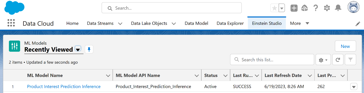
Use the Salesforce Einstein Studio API for predictions
Salesforce Einstein Studio is a new and centralized experience in Salesforce Data Cloud that data science and engineering teams can use to easily access their traditional models and LLMs used in generative AI. Next, we set up the API URL and client_id that you set in Secrets Manager earlier in Salesforce Einstein Studio to register and use the model inferences in Salesforce Einstein Studio. For instructions, refer to Bring Your Own AI Models to Salesforce with Einstein Studio.
Clean up
To delete all the resources created by the SageMaker project, on the project page, choose the Action menu and choose Delete.

To delete the resources (API Gateway and SageMaker endpoint) created by CodePipeline, navigate to the AWS CloudFormation console and delete the stack that was created.

Conclusion
In this post, we explained how you can build and train ML models in SageMaker Studio using SageMaker Data Wrangler to import and prepare data that is hosted on the Salesforce Data Cloud and use the newly launched Salesforce Data Cloud JDBC connector in SageMaker Data Wrangler and first-party Salesforce template in the SageMaker provided project template for Salesforce Data Cloud integration. The SageMaker project template for Salesforce enables you to deploy the model and create the endpoint and secure an API for a registered model. You then use the API to make predictions in Salesforce Einstein Studio for your business use cases.
Although we used the example of product recommendation to showcase the steps for implementing the end-to-end integration, you can use the SageMaker project template for Salesforce to create an endpoint and API for any SageMaker traditional model and LLM that is registered in the SageMaker Model Registry. We look forward to seeing what you build in SageMaker using data from Salesforce Data Cloud and empower your Salesforce applications using SageMaker hosted ML models!
This post is a continuation of the series regarding Salesforce Data Cloud and SageMaker integration. For a high-level overview and to learn more about the business impact you can make with this integration approach, refer to Part 1.
Additional resources
About the authors
 Daryl Martis is the Director of Product for Einstein Studio at Salesforce Data Cloud. He has over 10 years of experience in planning, building, launching, and managing world-class solutions for enterprise customers including AI/ML and cloud solutions. He has previously worked in the financial services industry in New York City. Follow him on https://www.linkedin.com/in/darylmartis.
 Rachna Chadha is a Principal Solutions Architect AI/ML in Strategic Accounts at AWS. Rachna is an optimist who believes that ethical and responsible use of AI can improve society in the future and bring economic and social prosperity. In her spare time, Rachna likes spending time with her family, hiking, and listening to music.
 Ife Stewart is a Principal Solutions Architect in the Strategic ISV segment at AWS. She has been engaged with Salesforce Data Cloud over the last 2 years to help build integrated customer experiences across Salesforce and AWS. Ife has over 10 years of experience in technology. She is an advocate for diversity and inclusion in the technology field.
 Dharmendra Kumar Rai (DK Rai) is a Sr. Data Architect, Data Lake & AI/ML, serving strategic customers. He works closely with customers to understand how AWS can help them solve problems, especially in the AI/ML and analytics space. DK has many years of experience in building data-intensive solutions across a range of industry verticals, including high-tech, FinTech, insurance, and consumer-facing applications.
 Marc Karp is an ML Architect with the SageMaker Service team. He focuses on helping customers design, deploy, and manage ML workloads at scale. In his spare time, he enjoys traveling and exploring new places.


 Daryl Martis is the Director of Product for Einstein Studio at Salesforce Data Cloud. He has over 10 years of experience in planning, building, launching, and managing world-class solutions for enterprise customers including AI/ML and cloud solutions. He has previously worked in the financial services industry in New York City.
 Maninder (Mani) Kaur is the AI/ML Specialist lead for Strategic ISVs at AWS. With her customer-first approach, Mani helps strategic customers shape their AI/ML strategy, fuel innovation, and accelerate their AI/ML journey. Mani is a firm believer of ethical and responsible AI, and strives to ensure that her customers’ AI solutions align with these principles.


 Sonali Sahu is leading intelligent document processing with the AI/ML services team in AWS. She is an author, thought leader, and passionate technologist. Her core area of focus is AI and ML, and she frequently speaks at AI and ML conferences and meetups around the world. She has both breadth and depth of experience in technology and the technology industry, with industry expertise in healthcare, the financial sector, and insurance.
 Ashish Lal is a Senior Product Marketing Manager who leads product marketing for AI services at AWS. He has 9 years of marketing experience and has led the product marketing effort for Intelligent document processing. He got his Master’s in Business Administration at the University of Washington.
 Mrunal Daftari is an Enterprise Senior Solutions Architect at Amazon Web Services. He is based in Boston, MA. He is a cloud enthusiast and very passionate about finding solutions for customers that are simple and address their business outcomes. He loves working with cloud technologies, providing simple, scalable solutions that drive positive business outcomes, cloud adoption strategy, and design innovative solutions and drive operational excellence.
 Dhiraj Mahapatro is a Principal Serverless Specialist Solutions Architect at AWS. He specializes in helping enterprise financial services adopt serverless and event-driven architectures to modernize their applications and accelerate their pace of innovation. Recently, he has been working on bringing container workloads and practical usage of generative AI closer to serverless and EDA for financial services industry customers.
 Jacob Hauskens is a Principal AI Specialist with over 15 years of strategic business development and partnerships experience. For the past 7 years, he has led the creation and implementation of go-to-market strategies for new AI-powered B2B services. Recently, he has been helping ISVs grow their revenue by adding generative AI to intelligent document processing workflows.
 Davide Gallitelli is a Specialist Solutions Architect for AI/ML in the EMEA region. He is based in Brussels and works closely with customers throughout Benelux. He has been a developer since he was very young, starting to code at the age of 7. He started learning AI/ML at university, and has fallen in love with it since then.
 Maurits de Groot is a Solutions Architect at Amazon Web Services, based out of Amsterdam. He likes to work on machine learning-related topics and has a predilection for startups. In his spare time, he enjoys skiing and playing squash.
 Peter Chung is a Solutions Architect for AWS, and is passionate about helping customers uncover insights from their data. He has been building solutions to help organizations make data-driven decisions in both the public and private sectors. He holds all AWS certifications as well as two GCP certifications. He enjoys coffee, cooking, staying active, and spending time with his family.
 Tim Song is a Software Development Engineer at AWS SageMaker, with 10+ years of experience as software developer, consultant and tech leader he has demonstrated ability to deliver scalable and reliable products and solve complex problems. In his spare time, he enjoys the nature, outdoor running, hiking and etc.
 Hariharan Suresh is a Senior Solutions Architect at AWS. He is passionate about databases, machine learning, and designing innovative solutions. Prior to joining AWS, Hariharan was a product architect, core banking implementation specialist, and developer, and worked with BFSI organizations for over 11 years. Outside of technology, he enjoys paragliding and cycling.
 Maia Haile is a Solutions Architect at Amazon Web Services based in the Washington, D.C. area. In that role, she helps public sector customers achieve their mission objectives with well architected solutions on AWS. She has 5 years of experience spanning from nonprofit healthcare, Media and Entertainment, and retail. Her passion is leveraging intelligence (AI) and machine learning (ML) to help Public Sector customers achieve their business and technical goals.
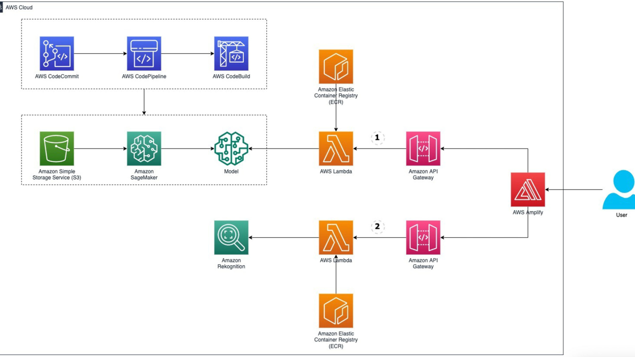


 Michael Wallner is a Senior Consultant Data & AI with AWS Professional Services and is passionate about enabling customers on their journey to become data-driven and AWSome in the AWS cloud. On top, he likes thinking big with customers to innovate and invent new ideas for them.
 David Sauerwein is a Senior Data Scientist at AWS Professional Services, where he enables customers on their AI/ML journey on the AWS cloud. David focuses on digital twins, forecasting and quantum computation. He has a PhD in theoretical physics from the University of Innsbruck, Austria. He was also a doctoral and post-doctoral researcher at the Max-Planck-Institute for Quantum Optics in Germany. In his free time he loves to read, ski and spend time with his family.
 Srikrishna Chaitanya Konduru is a Senior Data Scientist with AWS Professional services. He supports customers in prototyping and operationalising their ML applications on AWS. Srikrishna focuses on computer vision and NLP. He also leads ML platform design and use case identification initiatives for customers across diverse industry verticals. Srikrishna has an M.Sc in Biomedical Engineering from RWTH Aachen university, Germany, with a focus on Medical Imaging.
 Ahmed Mansour is a Data Scientist at AWS Professional Services. He provide technical support for customers through their AI/ML journey on the AWS cloud. Ahmed focuses on applications of NLP to the protein domain along with RL. He has a PhD in Engineering from the Technical University of Munich, Germany. In his free time he loves to go to the gym and play with his kids.


 Simon Zamarin is an AI/ML Solutions Architect whose main focus is helping customers extract value from their data assets. In his spare time, Simon enjoys spending time with family, reading sci-fi, and working on various DIY house projects.
 Saurabh Trikande is a Senior Product Manager for Amazon SageMaker Inference. He is passionate about working with customers and is motivated by the goal of democratizing machine learning. He focuses on core challenges related to deploying complex ML applications, multi-tenant ML models, cost optimizations, and making deployment of deep learning models more accessible. In his spare time, Saurabh enjoys hiking, learning about innovative technologies, following TechCrunch and spending time with his family.
 Durga Sury is an ML Solutions Architect in the Amazon SageMaker Service SA team. She is passionate about making machine learning accessible to everyone. In her 4 years at AWS, she has helped set up AI/ML platforms for enterprise customers. When she isn’t working, she loves motorcycle rides, mystery novels, and hiking with her 5-year-old husky.
 Ketan Vijayvargiya is a Senior Software Development Engineer in Amazon Web Services (AWS). His focus areas are machine learning, distributed systems and open source. Outside work, he likes to spend his time self-hosting and enjoying nature.