Artificial intelligence (AI) adoption is accelerating across industries and use cases. Recent scientific breakthroughs in deep learning (DL), large language models (LLMs), and generative AI is allowing customers to use advanced state-of-the-art solutions with almost human-like performance. These complex models often require hardware acceleration because it enables not only faster training but also faster inference when using deep neural networks in real-time applications. GPUs’ large number of parallel processing cores makes them well-suited for these DL tasks.
However, in addition to model invocation, those DL application often entail preprocessing or postprocessing in an inference pipeline. For example, input images for an object detection use case might need to be resized or cropped before being served to a computer vision model, or tokenization of text inputs before being used in an LLM. NVIDIA Triton is an open-source inference server that enables users to define such inference pipelines as an ensemble of models in the form of a Directed Acyclic Graph (DAG). It is designed to run models at scale on both CPU and GPU. Amazon SageMaker supports deploying Triton seamlessly, allowing you to use Triton’s features while also benefiting from SageMaker capabilities: a managed, secured environment with MLOps tools integration, automatic scaling of hosted models, and more.
AWS, in its dedication to help customers achieve the highest saving, has continuously innovated not only in pricing options and cost-optimization proactive services, but also in launching cost savings features like multi-model endpoints (MMEs). MMEs are a cost-effective solution for deploying a large number of models using the same fleet of resources and a shared serving container to host all of your models. Instead of using multiple single-model endpoints, you can reduce your hosting costs by deploying multiple models while paying only for a single inference environment. Additionally, MMEs reduce deployment overhead because SageMaker manages loading models in memory and scaling them based on the traffic patterns to your endpoint.
In this post, we show how to run multiple deep learning ensemble models on a GPU instance with a SageMaker MME. To follow along with this example, you can find the code on the public SageMaker examples repository.
How SageMaker MMEs with GPU work
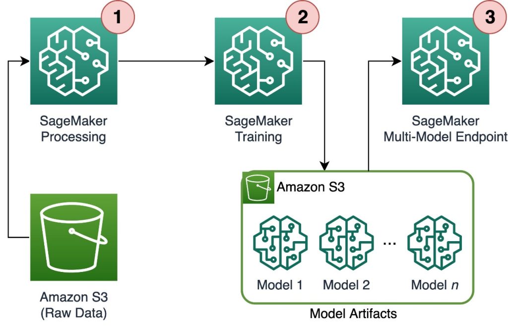
With MMEs, a single container hosts multiple models. SageMaker controls the lifecycle of models hosted on the MME by loading and unloading them into the container’s memory. Instead of downloading all the models to the endpoint instance, SageMaker dynamically loads and caches the models as they are invoked.
When an invocation request for a particular model is made, SageMaker does the following:
- It first routes the request to the endpoint instance.
- If the model has not been loaded, it downloads the model artifact from Amazon Simple Storage Service (Amazon S3) to that instance’s Amazon Elastic Block Storage volume (Amazon EBS).
- It loads the model to the container’s memory on the GPU-accelerated compute instance. If the model is already loaded in the container’s memory, invocation is faster because no further steps are needed.
When an additional model needs to be loaded, and the instance’s memory utilization is high, SageMaker will unload unused models from that instance’s container to ensure that there is enough memory. These unloaded models will remain on the instance’s EBS volume so that they can be loaded into the container’s memory later, thereby removing the need to download them again from the S3 bucket. However, If the instance’s storage volume reaches its capacity, SageMaker will delete the unused models from the storage volume. In cases where the MME receives many invocation requests, and additional instances (or an auto-scaling policy) are in place, SageMaker routes some requests to other instances in the inference cluster to accommodate for the high traffic.
This not only provides a cost saving mechanism, but also enables you to dynamically deploy new models and deprecate old ones. To add a new model, you upload it to the S3 bucket the MME is configured to use and invoke it. To delete a model, stop sending requests and delete it from the S3 bucket. Adding models or deleting them from an MME doesn’t require updating the endpoint itself!
Triton ensembles
The Triton model ensemble represents a pipeline that consists of one model, preprocessing and postprocessing logic, and the connection of input and output tensors between them. A single inference request to an ensemble triggers the run of the entire pipeline as a series of steps using the ensemble scheduler. The scheduler collects the output tensors in each step and provides them as input tensors for other steps according to the specification. To clarify: the ensemble model is still viewed as a single model from an external view.
Triton server architecture includes a model repository: a file system-based repository of the models that Triton will make available for inferencing. Triton can access models from one or more locally accessible file paths or from remote locations like Amazon S3.
Each model in a model repository must include a model configuration that provides required and optional information about the model. Typically, this configuration is provided in a config.pbtxt file specified as ModelConfig protobuf. A minimal model configuration must specify the platform or backend (like PyTorch or TensorFlow), the max_batch_size property, and the input and output tensors of the model.
Triton on SageMaker
SageMaker enables model deployment using Triton server with custom code. This functionality is available through the SageMaker managed Triton Inference Server Containers. These containers support common machine leaning (ML) frameworks (like TensorFlow, ONNX, and PyTorch, as well as custom model formats) and useful environment variables that let you optimize performance on SageMaker. Using SageMaker Deep Learning Containers (DLC) images is recommended because they’re maintained and regularly updated with security patches.
Solution walkthrough
For this post, we deploy two different types of ensembles on a GPU instance, using Triton and a single SageMaker endpoint.
The first ensemble consists of two models: a DALI model for image preprocessing and a TensorFlow Inception v3 model for actual inference. The pipeline ensemble takes encoded images as an input, which will have to be decoded, resized to 299×299 resolution, and normalized. This preprocessing will be handled by the DALI model. DALI is an open-source library for common image and speech preprocessing tasks such as decoding and data augmentation. Inception v3 is an image recognition model that consists of symmetric and asymmetric convolutions, and average and max pooling fully connected layers (and therefore is perfect for GPU usage).
The second ensemble transforms raw natural language sentences into embeddings and consists of three models. First, a preprocessing model is applied to the input text tokenization (implemented in Python). Then we use a pre-trained BERT (uncased) model from the Hugging Face Model Hub to extract token embeddings. BERT is an English language model that was trained using a masked language modeling (MLM) objective. Finally, we apply a postprocessing model where the raw token embeddings from the previous step are combined into sentence embeddings.
After we configure Triton to use these ensembles, we show how to configure and run the SageMaker MME.
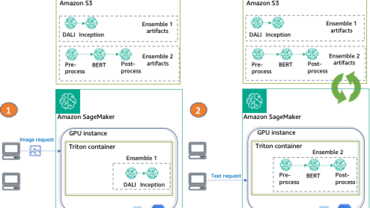
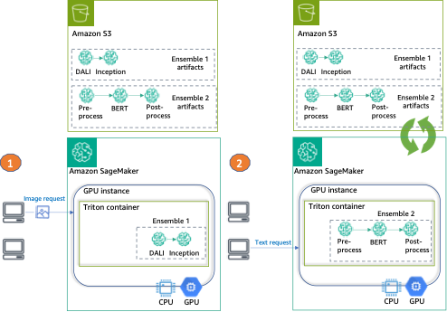
Finally, we provide an example of each ensemble invocation, as can be seen in the following diagram:
- Ensemble 1 – Invoke the endpoint with an image, specifying DALI-Inception as the target ensemble
- Ensemble 2 – Invoke the same endpoint, this time with text input and requesting the preprocess-BERT-postprocess ensemble
Set up the environment
First, we set up the needed environment. This includes updating AWS libraries (like Boto3 and the SageMaker SDK) and installing the dependencies required to package our ensembles and run inferences using Triton. We also use the SageMaker SDK default execution role. We use this role to enable SageMaker to access Amazon S3 (where our model artifacts are stored) and the container registry (where the NVIDIA Triton image will be used from). See the following code:
Prepare ensembles
In this next step, we prepare the two ensembles: the TensorFlow (TF) Inception with DALI preprocessing and BERT with Python preprocessing and postprocessing.
This entails downloading the pre-trained models, providing the Triton configuration files, and packaging the artifacts to be stored in Amazon S3 before deploying.
Prepare the TF and DALI ensemble
First, we prepare the directories for storing our models and configurations: for the TF Inception (inception_graphdef), for DALI preprocessing (dali), and for the ensemble (ensemble_dali_inception). Because Triton supports model versioning, we also add the model version to the directory path (denoted as 1 because we only have one version). To learn more about the Triton version policy, refer to Version Policy. Next, we download the Inception v3 model, extract it, and copy to the inception_graphdef model directory. See the following code:
Now, we configure Triton to use our ensemble pipeline. In a config.pbtxt file, we specify the input and output tensor shapes and types, and the steps the Triton scheduler needs to take (DALI preprocessing and the Inception model for image classification):
Next, we configure each of the models. First, the model config for DALI backend:
Next, the model configuration for TensorFlow Inception v3 we downloaded earlier:
Because this is a classification model, we also need to copy the Inception model labels to the inception_graphdef directory in the model repository. These labels include 1,000 class labels from the ImageNet dataset.
Next, we configure and serialize the DALI pipeline that will handle our preprocessing to file. The preprocessing includes reading the image (using CPU), decoding (accelerated using GPU), and resizing and normalizing the image.
Finally, we package the artifacts together and upload them as a single object to Amazon S3:
Prepare the TensorRT and Python ensemble
For this example, we use a pre-trained model from the transformers library.
You can find all models (preprocess and postprocess, along with config.pbtxt files) in the folder ensemble_hf. Our file system structure will include four directories (three for the individual model steps and one for the ensemble) as well as their respective versions:
In the workspace folder, we provide with two scripts: the first to convert the model into ONNX format (onnx_exporter.py) and the TensorRT compilation script (generate_model_trt.sh).
Triton natively supports the TensorRT runtime, which enables you to easily deploy a TensorRT engine, thereby optimizing for a selected GPU architecture.
To make sure we use the TensorRT version and dependencies that are compatible with the ones in our Triton container, we compile the model using the corresponding version of NVIDIA’s PyTorch container image:
We then copy the model artifacts to the directory we created earlier and add a version to the path:
We use a Conda pack to generate a Conda environment that the Triton Python backend will use in preprocessing and postprocessing:
Finally, we upload the model artifacts to Amazon S3:
Run ensembles on a SageMaker MME GPU instance
Now that our ensemble artifacts are stored in Amazon S3, we can configure and launch the SageMaker MME.
We start by retrieving the container image URI for the Triton DLC image that matches the one in our Region’s container registry (and is used for TensorRT model compilation):
Next, we create the model in SageMaker. In the create_model request, we describe the container to use and the location of model artifacts, and we specify using the Mode parameter that this is a multi-model.
To host our ensembles, we create an endpoint configuration with the create_endpoint_config API call, and then create an endpoint with the create_endpoint API. SageMaker then deploys all the containers that you defined for the model in the hosting environment.
Although in this example we are setting a single instance to host our model, SageMaker MMEs fully support setting an auto scaling policy. For more information on this feature, see Run multiple deep learning models on GPU with Amazon SageMaker multi-model endpoints.
Create request payloads and invoke the MME for each model
After our real-time MME is deployed, it’s time to invoke our endpoint with each of the model ensembles we used.
First, we create a payload for the DALI-Inception ensemble. We use the shiba_inu_dog.jpg image from the SageMaker public dataset of pet images. We load the image as an encoded array of bytes to use in the DALI backend (to learn more, see Image Decoder examples).
With our encoded image and payload ready, we invoke the endpoint.
Note that we specify our target ensemble to be the model_tf_dali.tar.gz artifact. The TargetModel parameter is what differentiates MMEs from single-model endpoints and enables us to direct the request to the right model.
The response includes metadata about the invocation (such as model name and version) and the actual inference response in the data part of the output object. In this example, we get an array of 1,001 values, where each value is the probability of the class the image belongs to (1,000 classes and 1 extra for others).
Next, we invoke our MME again, but this time target the second ensemble. Here the data is just two simple text sentences:
To simplify communication with Triton, the Triton project provides several client libraries. We use that library to prepare the payload in our request:
Now we are ready to invoke the endpoint—this time, the target model is the model_trt_python.tar.gz ensemble:
The response is the sentence embeddings that can be used in a variety of natural language processing (NLP) applications.
Clean up
Lastly, we clean up and delete the endpoint, endpoint configuration, and model:
Conclusion
In this post, we showed how to configure, deploy, and invoke a SageMaker MME with Triton ensembles on a GPU-accelerated instance. We hosted two ensembles on a single real-time inference environment, which reduced our cost by 50% (for a g4dn.4xlarge instance, which represents over $13,000 in yearly savings). Although this example used only two pipelines, SageMaker MMEs can support thousands of model ensembles, making it an extraordinary cost savings mechanism. Furthermore, you can use SageMaker MMEs’ dynamic ability to load (and unload) models to minimize the operational overhead of managing model deployments in production.
About the authors
 Saurabh Trikande is a Senior Product Manager for Amazon SageMaker Inference. He is passionate about working with customers and is motivated by the goal of democratizing machine learning. He focuses on core challenges related to deploying complex ML applications, multi-tenant ML models, cost optimizations, and making deployment of deep learning models more accessible. In his spare time, Saurabh enjoys hiking, learning about innovative technologies, following TechCrunch, and spending time with his family.
 Nikhil Kulkarni is a software developer with AWS Machine Learning, focusing on making machine learning workloads more performant on the cloud, and is a co-creator of AWS Deep Learning Containers for training and inference. He’s passionate about distributed Deep Learning Systems. Outside of work, he enjoys reading books, fiddling with the guitar, and making pizza.
 Uri Rosenberg is the AI & ML Specialist Technical Manager for Europe, Middle East, and Africa. Based out of Israel, Uri works to empower enterprise customers to design, build, and operate ML workloads at scale. In his spare time, he enjoys cycling, backpacking, and backpropagating.
 Eliuth Triana Isaza is a Developer Relations Manager on the NVIDIA-AWS team. He connects Amazon and AWS product leaders, developers, and scientists with NVIDIA technologists and product leaders to accelerate Amazon ML/DL workloads, EC2 products, and AWS AI services. In addition, Eliuth is a passionate mountain biker, skier, and poker player.
 James Poquiz is a Data Scientist with AWS Professional Services based in Orange County, California. He has a BS in Computer Science from the University of California, Irvine and has several years of experience working in the data domain having played many different roles. Today he works on implementing and deploying scalable ML solutions to achieve business outcomes for AWS clients.
 Han Man is a Senior Data Science & Machine Learning Manager with AWS Professional Services based in San Diego, CA. He has a PhD in Engineering from Northwestern University and has several years of experience as a management consultant advising clients in manufacturing, financial services, and energy. Today, he is passionately working with key customers from a variety of industry verticals to develop and implement ML and GenAI solutions on AWS.
 Safa Tinaztepe is a full-stack data scientist with AWS Professional Services. He has a BS in computer science from Emory University and has interests in MLOps, distributed systems, and web3.


 Munish Dabra is a Principal Solutions Architect at Amazon Web Services (AWS). His current areas of focus are AI/ML and Observability. He has a strong background in designing and building scalable distributed systems. He enjoys helping customers innovate and transform their business in AWS. LinkedIn:
  Patrick Lin is a Software Development Engineer with Amazon SageMaker Data Wrangler. He is committed to making Amazon SageMaker Data Wrangler the number one data preparation tool for productionized ML workflows. Outside of work, you can find him reading, listening to music, having conversations with friends, and serving at his church.


 Arun Anand is a Senior Solutions Architect at Amazon Web Services based in Houston area. He has 25+ years of experience in designing and developing enterprise applications. He works with partners in Energy & Utilities segment providing architectural and best practice recommendations for new and existing solutions.
 Rajnish Shaw is a Senior Solutions Architect at Amazon Web Services, with a background as a Product Developer and Architect. Rajnish is passionate about helping customers build applications on the cloud. Outside of work Rajnish enjoys spending time with family and friends, and traveling.
 Yuanhua Wang is a software engineer at AWS with more than 15 years of experience in the technology industry. His interests are software architecture and build tools on cloud computing.


 Daryl Martis is the Director of Product for Einstein Studio at Salesforce Data Cloud. He has over 10 years of experience in planning, building, launching, and managing world-class solutions for enterprise customers including AI/ML and cloud solutions. He has previously worked in the financial services industry in New York City. Follow him on
  Rachna Chadha is a Principal Solutions Architect AI/ML in Strategic Accounts at AWS. Rachna is an optimist who believes that ethical and responsible use of AI can improve society in the future and bring economic and social prosperity. In her spare time, Rachna likes spending time with her family, hiking, and listening to music.
 Ife Stewart is a Principal Solutions Architect in the Strategic ISV segment at AWS. She has been engaged with Salesforce Data Cloud over the last 2 years to help build integrated customer experiences across Salesforce and AWS. Ife has over 10 years of experience in technology. She is an advocate for diversity and inclusion in the technology field.
 Dharmendra Kumar Rai (DK Rai) is a Sr. Data Architect, Data Lake & AI/ML, serving strategic customers. He works closely with customers to understand how AWS can help them solve problems, especially in the AI/ML and analytics space. DK has many years of experience in building data-intensive solutions across a range of industry verticals, including high-tech, FinTech, insurance, and consumer-facing applications.
 Marc Karp is an ML Architect with the SageMaker Service team. He focuses on helping customers design, deploy, and manage ML workloads at scale. In his spare time, he enjoys traveling and exploring new places.


 Daryl Martis is the Director of Product for Einstein Studio at Salesforce Data Cloud. He has over 10 years of experience in planning, building, launching, and managing world-class solutions for enterprise customers including AI/ML and cloud solutions. He has previously worked in the financial services industry in New York City.
 Maninder (Mani) Kaur is the AI/ML Specialist lead for Strategic ISVs at AWS. With her customer-first approach, Mani helps strategic customers shape their AI/ML strategy, fuel innovation, and accelerate their AI/ML journey. Mani is a firm believer of ethical and responsible AI, and strives to ensure that her customers’ AI solutions align with these principles.


 Sonali Sahu is leading intelligent document processing with the AI/ML services team in AWS. She is an author, thought leader, and passionate technologist. Her core area of focus is AI and ML, and she frequently speaks at AI and ML conferences and meetups around the world. She has both breadth and depth of experience in technology and the technology industry, with industry expertise in healthcare, the financial sector, and insurance.
 Ashish Lal is a Senior Product Marketing Manager who leads product marketing for AI services at AWS. He has 9 years of marketing experience and has led the product marketing effort for Intelligent document processing. He got his Master’s in Business Administration at the University of Washington.
 Mrunal Daftari is an Enterprise Senior Solutions Architect at Amazon Web Services. He is based in Boston, MA. He is a cloud enthusiast and very passionate about finding solutions for customers that are simple and address their business outcomes. He loves working with cloud technologies, providing simple, scalable solutions that drive positive business outcomes, cloud adoption strategy, and design innovative solutions and drive operational excellence.
 Dhiraj Mahapatro is a Principal Serverless Specialist Solutions Architect at AWS. He specializes in helping enterprise financial services adopt serverless and event-driven architectures to modernize their applications and accelerate their pace of innovation. Recently, he has been working on bringing container workloads and practical usage of generative AI closer to serverless and EDA for financial services industry customers.
 Jacob Hauskens is a Principal AI Specialist with over 15 years of strategic business development and partnerships experience. For the past 7 years, he has led the creation and implementation of go-to-market strategies for new AI-powered B2B services. Recently, he has been helping ISVs grow their revenue by adding generative AI to intelligent document processing workflows.
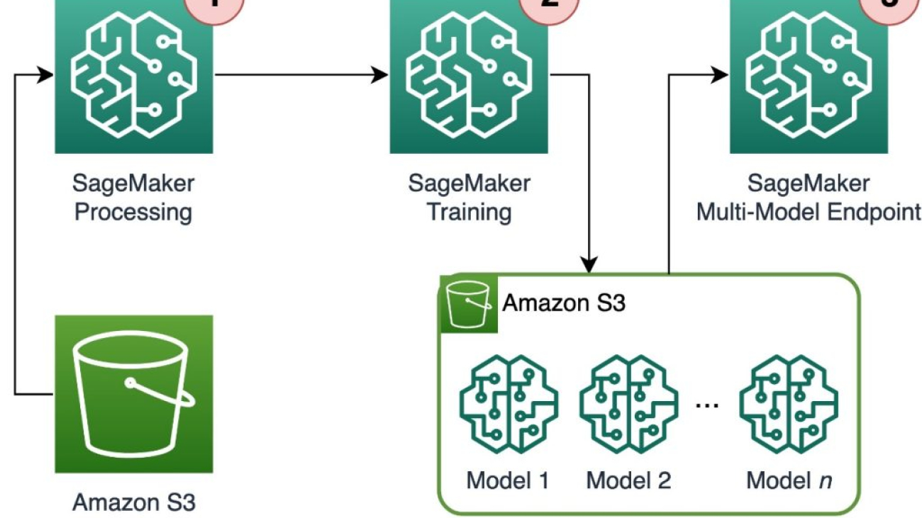
 Davide Gallitelli is a Specialist Solutions Architect for AI/ML in the EMEA region. He is based in Brussels and works closely with customers throughout Benelux. He has been a developer since he was very young, starting to code at the age of 7. He started learning AI/ML at university, and has fallen in love with it since then.
 Maurits de Groot is a Solutions Architect at Amazon Web Services, based out of Amsterdam. He likes to work on machine learning-related topics and has a predilection for startups. In his spare time, he enjoys skiing and playing squash.